Modern Control Theory
Zdzislaw Bubnicki
Modern Control Theory
With 104 figures
Wroclaw University of Technology
Institute of Information Science and Engineering Wyb. Wyspianskiego 27
50-370 Wroclaw Poland
Library of Congress Control Number: 2005925392
ISBN 10 3-540-23951-0 Springer Berlin Heidelberg New York ISBN 13 978-3-540-23951-2 Springer Berlin Heidelberg New York
This work is subject to copyright. All rights are reserved, whether the whole or part of the material is concerned, specifically the rights of translation, reprinting, reuse of illustrations, recitation, broadcasting, reproduction on microfilm or in other ways, and storage in data banks. Duplication of this publication or parts thereof is permitted only under the provisions of the German Copyright Law of September 9, 1965, in its current version, and permission for use must always be obtained from Springer-Verlag. Violations are liable to prosecution under German Copyright Law.
Springer is a part of Springer Science+Business Media springeronline.com
© Springer-Verlag Berlin Heidelberg 2005 Printed in Germany
The use of general descriptive names, registered names, trademarks, etc. in this publication does not imply, even in the absence of a specific statement, that such names are exempt from the relevant protective laws and regulations and therefore free for general use.
Typesetting: Data conversion by the author.
Final processing by PTP-Berlin Protago-TEX-Production GmbH, Germany Cover-Design: Medionet AG, Berlin
Printed on acid-free paper 89/3141/Yu – 5 4 3 2 1 0
Originally published in Polish by Polish Scientifi c Publishers PWN, 2002
Preface
The main aim of this book is to present a unified, systematic description of basic and advanced problems, methods and algorithms of the modern con-trol theory considered as a foundation for the design of computer concon-trol and management systems. The scope of the book differs considerably from the topics of classical traditional control theory mainly oriented to the needs of automatic control of technical devices and technological proc-esses. Taking into account a variety of new applications, the book presents a compact and uniform description containing traditional analysis and op-timization problems for control systems as well as control problems with non-probabilistic models of uncertainty, problems of learning, intelligent, knowledge-based and operation systems – important for applications in the control of manufacturing processes, in the project management and in the control of computer systems. Into the uniform framework of the book, original ideas and results based on the author’s works concerning uncertain and intelligent knowledge-based control systems, applications of uncertain variables and the control of complexes of operations have been included. The material presented in the book is self-contained. Using the text does not require any earlier knowledge on the control science. The presentation requires only a basic knowledge of linear algebra, differential equations and probability theory. I hope that the book can be useful for students, re-searches and all readers working in the field of control and information science and engineering.
I wish to express my gratitude to Dr. D. Orski and Dr. L. Siwek, my co-workers at the Institute of Information Science and Engineering of Wro-claw University of Technology, who assisted in the preparation of the manuscript.
1 General Characteristic of Control Systems...1
1.1 Subjectand Scope of Control Theory...1
1.2 Basic Terms ...2
1.2.1 Control Plant ...4
1.2.2 Controller ...6
1.3 Classification of Control Systems...7
1.3.1 Classification with Respect to Connection Between Plant and Controller ...7
1.3.2 Classification with Respect to Control Goal...9
1.3.3 Other Cases ...11
1.4 Stages of Control System Design ...13
1.5 Relations Between Control Science and Related Areas in Science and Technology ...14
1.6 Character, Scope and Composition of the Book...15
2 Formal Models of Control Systems ...17
2.1 Description of a Signal ...17
2.2 Static Plant ...18
2.3 Continuous Dynamical Plant ...19
2.3.1 State Vector Description ...20
2.3.2 “Input-output” Description by Means of Differential Equation24 2.3.3 Operational Form of “Input-output” Description...25
2.4 Discrete Dynamical Plant ...29
2.5 Control Algorithm ...31
2.6 Introduction to Control System Analysis...33
2.6.1 Continuous System ...35
2.6.2 Discrete System ...37
3 Control for the Given State (the Given Output)...41
3.1 Control of a Static Plant...41
3.2 Control of a Dynamical Plant. Controllability...44
3.3 Control of a Measurable Plant in the Closed-loop System ...47
VIII Contents
3.5 Control with an Observer in the Closed-loop System ...55
3.6 Structural Approach...59
3.7 Additional Remarks ...62
4 Optimal Control with Complete Information on the Plant ...65
4.1 Control of a Static Plant...65
4.2 Problems of Optimal Control for Dynamical Plants...69
4.2.1 Discrete Plant...69
4.2.2 Continuous Plant...72
4.3 Principle of Optimality and Dynamic Programming ...74
4.4 Bellman Equation ...79
4.5 Maximum Principle ...85
4.6 Linear-quadratic Problem ...93
5 Parametric Optimization ...97
5.1 General Idea of Parametric Optimization ...97
5.2 Continuous Linear Control System...99
5.3 Discrete Linear Control System...105
5.4 System with the Measurement of Disturbances...107
5.5 Typical Forms of Control Algorithms in Closed-loop Systems ....110
5.5.1 Linear Controller...111
5.5.2 Two-position Controller ...112
5.5.3 Neuron-like Controller...112
5.5.4 Fuzzy Controller ...113
6 Application of Relational Description of Uncertainty ...117
6.1 Uncertainty and Relational Knowledge Representation ...117
6.2 Analysis Problem...122
6.3 Decision Making Problem ...127
6.4 Dynamical Relational Plant ...130
6.5 Determinization ...136
7 Application of Probabilistic Descriptions of Uncertainty...143
7.1 Basic Problems for Static Plant and Parametric Uncertainty...143
7.2 Basic Problems for Static Plant and Non-parametric Uncertainty 152 7.3 Control of Static Plant Using Results of Observations...157
7.3.1 Indirect Approach ...158
7.3.2 Direct Approach...164
7.4 Application of Games Theory...165
7.5 Basic Problem for Dynamical Plant...170
7.7 Analysis and Parametric Optimization of Linear Closed-loop
Control System with Stationary Stochastic Disturbances...178
7.8 Non-parametric Optimization of Linear Closed-loop Control System with Stationary Stochastic Disturbances...183
7.9 Relational Plant with Random Parameter ...188
8 Uncertain Variables and Their Applications...193
8.1 Uncertain Variables ...193
8.2 Application of Uncertain Variables to Analysis and Decision Making (Control) for Static Plant ...201
8.2.1 Parametric Uncertainty ...201
8.2.2 Non-parametric Uncertainty ...205
8.3 Relational Plant with Uncertain Parameter...211
8.4 Control for Dynamical Plants. Uncertain Controller ...216
9 Fuzzy Variables, Analogies and Soft Variables ...221
9.1 Fuzzy Sets and Fuzzy Numbers...221
9.2 Application of Fuzzy Description to Decision Making (Control) for Static Plant ...228
9.2.1 Plant without Disturbances ...228
9.2.2 Plant with External Disturbances...233
9.3 Comparison of Uncertain Variables with Random and Fuzzy Variables ...238
9.4 Comparisons and Analogies for Non-parametric Problems ...242
9.5 Introduction to Soft Variables...246
9.6 Descriptive and Prescriptive Approaches. Quality of Decisions ...249
9.7 Control for Dynamical Plants. Fuzzy Controller ...255
10 Control in Closed-loop System. Stability ...259
10.1 General Problem Description...259
10.2 Stability Conditions for Linear Stationary System ...264
10.2.1 Continuous System ...264
10.2.2 Discrete System ...266
10.3 Stability of Non-linear and Non-stationary Discrete Systems ...270
10.4 Stability of Non-linear and Non-stationary Continuous Systems 277 10.5 Special Case. Describing Function Method...278
10.6 Stability of Uncertain Systems. Robustness ...282
10.7 An Approach Based on Random and Uncertain Variables...291
10.8 Convergence of Static Optimization Process...295
11 Adaptive and Learning Control Systems ...299
X Contents
11.2 Adaptation via Identification for Static Plant ...303
11.3 Adaptation via Identification for Dynamical Plant ...309
11.4 Adaptation via Adjustment of Controller Parameters...311
11.5 Learning Control System Based on Knowledge of the Plant...313
11.5.1 Knowledge Validation and Updating...314
11.5.2 Learning Algorithm for Decision Making in Closed-loop System...317
11.6 Learning Control System Based on Knowledge of Decisions....319
11.6.1 Knowledge Validation and Updating...319
11.6.2 Learning Algorithm for Control in Closed-loop System ...321
12 Intelligent and Complex Control Systems ...327
12.1 Introduction to Artificial Intelligence ...327
12.2 Logical Knowledge Representation...328
12.3 Analysis and Decision Making Problems ...332
12.4 Logic-algebraic Method...334
12.5 Neural Networks ...341
12.6 Applications of Neural Networks in Control Systems...346
12.6.1 Neural Network as a Controller ...346
12.6.2 Neural Network in Adaptive System ...348
12.7 Decomposition and Two-level Control...349
12.8 Control of Complex Plant with Cascade Structure ...355
12.9 Control of Plant with Two-level Knowledge Representation...358
13 Control of Operation Systems...363
13.1 General Characteristic...363
13.2 Control of Task Distribution...365
13.3 Control of Resource Distribution...371
13.4 Control of Assignment and Scheduling ...375
13.5 Control of Allocation in Systems with Transport ...382
13.6 Control of an Assembly Process...386
13.7 Application of Relational Description and Uncertain Variables .391 13.8 Application of Neural Network ...398
Conclusions...401
Appendix...405
References...411
1.1 Subject and Scope of Control Theory
The modern control theory is a discipline dealing with formal foundations of the analysis and design of computer control and management sys-tems. Its basic scope contains problems and methods of control algorithms design, where the control algorithms are understood as formal prescrip-tions (formulas, procedures, programs) for the determination of control de-cisions, which may be executed by technical devices able to the informa-tion processing and decision making. The problems and methods of the control theory are common for different executors of the control algo-rithms. Nowadays, they are most often computer devices and systems. The computer control and management systems or wider − decision support systems belong now to the most important, numerous and intensively de-veloping computer information systems. The control theory deals with the foundations, methods and decision making algorithms needed for develop-ing computer programs in such systems.
The problems and methods of the control theory are common not only for different executors of the control algorithms but also − which is per-haps more important – for various applications. In the first period, the con-trol theory has been developing mainly for the automatic control of techni-cal processes and devices. This area of applications is of course still important and developing, and the development of the information tech-nology has created new possibilities and – on the other hand – new prob-lems. The full automatization of the control contains also the automatiza-tion of manipulaautomatiza-tion operaautomatiza-tions, the control of executing mechanisms, intelligent tools and robots which may be objects of the external control and should contain inner controlling devices and systems.
2 1 General Characteristic of Control Systems
systematic way with problems concerning the different applications men-tioned here. The scope of this area significantly exceeds the framework of so called traditional (or classical) control theory. The needs and applica-tions mentioned above determine also new direcapplica-tions and perspectives of the future development of the modern control theory.
Summarizing the above remarks one can say that the control theory (or wider −control science) is a basic discipline for the automatic control and robotics and one of basic disciplines for the information technology and management. It provides the methods necessary to a rational design and ef-fective use of computer tools in the decision support systems and in par-ticular, in the largest class of such systems, namely in control and man-agement systems.
Additional remarks concerning the subject and the scope of the control theory will be presented in Sect. 1.2 after the description of basic terms, and in Sect. 1.5 characterizing interconnections between the control theory and other related areas.
1.2 Basic Terms
To characterize more precisely the term control let us consider the follow-ing examples:
1. Control (steering) of a vehicle movement so as to keep a required trajec-tory and velocity of the motion.
2. Control of an electrical furnace (the temperature control), consisting in changing the voltage put at the heater so as to stabilize the temperature at the required level in spite of the external temperature variations.
3. Stabilization of the temperature in a human body as a result of the action of inner steering organs.
4. Control of the medicine dosage in a given therapy in order to reach and keep required biomedical indexes.
8. Admission and congestion control in computer networks in order to keep good performance indexes concerning the service quality.
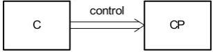
Generalizing these examples we can say that the control is defined as a goal-oriented action. With this action there is associated a certain object which is acted upon and a certain subject executing the action. In the fur-ther considerations the object will be called a control plant (CP) and the subject − a controller (C) or more precisely speaking, an executor of the control algorithm. Sometimes for the controller we use the term a control-ling system to indicate its complexity. The interconnection of these two ba-sic parts (the control plant and the controller) defines a control system. The way of interconnecting the basic parts and eventually some additional blocks determines the structure of the control system. Figure 1.1 illustrates the simplest structure of the control system in which the controller C con-trols the plant CP.
[image:11.439.144.298.253.291.2]C control CP
Fig. 1.1. Basic scheme of control system
Remark 1.1. Regardless different names (control, steering, management), the main idea of the control consists in decision making based on certain information, and the decisions are concerned with a certain plant. Usually, speaking about the control, we do not have in mind single one-stage deci-sions but a certain multistage decision process distributed in time. How-ever, it is not an essential feature of the control and it is often difficult to state in the case when separate independent decisions are made in succes-sive cycles with different data.
□
Remark 1.2. The control plant and the controller are imprecise terms in this sense that the control plant does not have to mean a determined object or device. For example, the control of a material flow in an enterprise does not mean the control of the enterprise as a determined plant. On the other hand, the controller should be understood as an executor of the control al-gorithm, regardless its practical nature which does not have to have a tech-nical character; in particular, it may be a human operator.
□
4 1 General Characteristic of Control Systems
1.2.1 Control Plant
An object of the control (a process, a system, or a device) is called a con-trol plant and treated uniformly regardless its nature and the degree of complexity. In the further considerations in this chapter we shall use the temperature control in an electrical furnace as a simple example to explain the basic ideas, having in mind that the control plants may be much more complicated and may be of various practical nature, not only technical. For example they may be different kinds of economical processes in the case of the management. In order to present a formal description we introduce variables characterizing the plant: controlled variables, controlling vari-ables and disturbances.
By controlled variables we define the variables used for the determina-tion of the control goal. In the case of the furnace it is a temperature in the furnace for which a required value is given; in the case of a production process it may be e.g. the productivity or a profit in a determined time in-terval. Usually, the controlled variables may be measured (or observed), and more generally – the information on their current values may be ob-tained by processing other information available. In the further considera-tions we shall use the word “to measure” just in such a generalized sense for the variables which are not directly measured. In complex plants a set of controlled variables may occur. They will be ordered and treated as components of a vector. For example, a turbogenerator in an electrical power station may have two controlled variables: the value and the fre-quency of the output voltage. In a certain production process, variables characterizing the product may be controlled variables.
By controlling variables (or control variables) we understand the vari-ables which can be changed or put from outside and which have impact on the controlled variables. Their values are the control decisions; the control is performed by the proper choosing and changing of these values. In the furnace it is the voltage put at the electrical heater, in the turbogenerator – a turbine velocity and the current in the rotor, in the production process – the size and parameters of a raw material.
We shall apply the following notations (Fig. 1.2)
u =
⎥ ⎥ ⎥ ⎥ ⎥ ⎦ ⎤ ⎢ ⎢ ⎢ ⎢ ⎢ ⎣ ⎡ ) ( ) 2 ( ) 1 ( p u u u
, y =
⎥ ⎥ ⎥ ⎥ ⎥ ⎦ ⎤ ⎢ ⎢ ⎢ ⎢ ⎢ ⎣ ⎡ ) ( ) 2 ( ) 1 ( l y y y
, z =
⎥ ⎥ ⎥ ⎥ ⎥ ⎦ ⎤ ⎢ ⎢ ⎢ ⎢ ⎢ ⎣ ⎡ ) ( ) 2 ( ) 1 ( r z z z
where u(i) − the i-th controlling variable, i=1,2,...,p; y(j) − the j-th con-trolled variable, j=1,2,...,l; z(m) − the m-th disturbance, m=1,2,...,r; u, y, z denote the controlling vector (or control vector), the controlled vector and the vector of the disturbances, respectively. The vectors are written as one-column matrices. CP y z u CP u(1) u(2)
u(p)
y(1)
y(2)
y(l) z(1)z(2) z(r)
. . .
... ...
Fig. 1.2. Control plant
6 1 General Characteristic of Control Systems
1.2.2 Controller
An executor of the control algorithm is called a controller C (controlling system, controlling device) and treated uniformly regardless its nature and the degree of complexity. It may be e.g. a human operator, a specialized so called analog device (e.g. analog electronic controller), a controlling com-puter, a complex controlling system consisting of cooperating computers, analog devices and human operators. The output vector of the controller is the control vector u and the components of the input vector are variables whose values are introduced into C as data used to finding the control de-cisions. They may be values taken from the plant, i.e. u and (or) z, or val-ues characterizing the external information. A control algorithm, i.e. the dependence of u upon w or a way of determining control decisions based on the input data, corresponds to the model of the plant, i.e. the depend-ence of y upon u and z. In simple cases it is a function u=Ψ(w), in more complicated cases − the relationship between the functions describing time-varying variables w and u. Formal descriptions of the control algo-rithm and the plant model may be the same. However, there are essential differences concerning the interpretation of the description and its obtain-ing. In the case of the plant, it is a formal description of an existing real unit, which may be obtained on the basis of observation. In the case of the controller, it is a prescription of an action, which is determined by a de-signer and then is executed by a determined subject of this action, e.g. by the controlling computer.
In the case of a full automatization possible for the control of technical processes and devices, the controlling system, except the executor of the control algorithm as a basic part, contains additional devices necessary for the acquisition and introducing the information, and for the execution of the decisions. In the case of a computer realization, they are additional de-vices linking the computer and the control plant (a specific interface in the computer control system). Technical problems connected with the design and exploitation of a computer control system exceed the framework of this book and belong to control system engineering and information tech-nology. It is worth, however, noting now that the computer control systems are real-time systems which means that introducing current data, finding the control decisions and bringing them out for execution should be per-formed in determined time intervals and if they are short (which occurs as a rule in the cases of a control of technical plants and processes, and in op-erating management), then the information processing and finding the cur-rent decisions should be respectively quick.
occur-ring here and the role of the control theory and engineeoccur-ring:
1. The control theory and engineering deal with methods and techniques common for the control of real plants with various practical nature. From the methodology of control algorithms determination point of view, the plants having different real nature but described by the same mathematical models are identical. To a certain degree, such a universalization concerns the executors of control algorithms as well (e.g. universal control com-puter). That is why, illustrating graphically the control systems, we present only blocks denoting parts or elements of the system, i.e. so called block-schemes as a universal illustration of real systems.
2. The basic practical effects or “utility products” of the control theory are control algorithms which are used as a basis for developing and imple-menting the corresponding computer programs or (nowadays, to a limited degree) for building specialized controlling devices. Methods of the con-trol theory enable a rational concon-trol algorithmization based on a plant model and precisely formulated requirements, unlike a control based on an undetermined experience and intuition of a human operator, which may give much worse effects. The algorithmization is necessary for the automa-tization (the computerization) of the control but in simple cases the control algorithm may be “hand-executed” by a human operator. For that reason, from the control theory and methodology point of view, the difference be-tween an algorithmized control and a control based on an imprecise ex-perience is much more essential than the difference between automatic and hand-executed control. The function of the control computer consists in the determination of control decisions which may be executed directly by a technical device and (or) by a human operator, or may be given for the execution by a manager. Usually, in the second case the final decision is made by a manager (generally, by a decision maker) and the computer sys-tem serves as an expert syssys-tem supporting the control process.
1.3 Classification of Control Systems
In this section we shall use the term classification, although in fact it will be the presentation of typical cases, not containing all possible situations.
1.3.1 Classification with Respect to Connection Between Plant and Controller
8 1 General Characteristic of Control Systems
can consider the following cases:
1. Open-loop system without the measurement of disturbances. 2. Open-loop system with the measurement of disturbances. 3. Closed-loop system.
4. Mixed (combined) system.
These concepts, illustrated in Figs. 1.3 and 1.4, differ from each other with the kind of information (if any) introduced into the executor of the control algorithm and used to the determination of control decisions.
C u CP y C CP
z z
z u y
a) b)
Fig. 1.3. Block schemes of open-loop control system: a) without measurement of disturbances, b) with measurement of disturbances
C CP
z
a)
u y
C CP
z
b)
u y
Fig. 1.4. Block schemes of control systems: a) closed-loop, b) mixed
means that e.g. increasing of the value y will cause a change of u resulting in decreasing of the value y. Additionally let us note that the variables oc-curring in a control system have a character of signals, i.e. variables con-taining and transferring information. Consequently, we can say that in the feed-back system a closed loop of the information transferring occurs. Comparing systems 2 and 3 we can generally say that in system 2 a much more precise knowledge of the plant, i.e. of its reaction to the actions u and z, is required. In system 3 the additional information on the plant is obtained via the observations of the control effects. Furthermore, in system
2 the control compensates the influence of the measured disturbances only, while in system 3 the influence on the observed effect y of all disturbances (not only not measured but also not determined) is compensated. However, not only the advantages but also the disadvantages of the concept 3 com-paring with the concept 2 should be taken into account: counteracting the changes of z may be much slower than in system 2 and, if the reactions on the difference between a real and a required value y are too intensive, the value of y may not converge to a steady state, which means that the control system does not behave in a stabilizing way. In the example of the furnace, after a step change of the outside temperature (in practice, after a very quick change of this temperature), the control will begin with a delay, only when the effect of this change is measured by the thermometer inside the furnace. Too great and quick changes of the voltage put on the heater, de-pending on the difference between the current temperature inside the fur-nace and the required value of this temperature, may cause oscillations of this difference with an increasing amplitude. The advantages of system 2
and 3 are combined into a properly designed mixed system which in the example with the furnace requires two thermometers – inside and outside the furnace.
1.3.2 Classification with Respect to Control Goal
Depending on the control goal formulation, two typical cases are usually considered:
1. Control system with the required output. 2. Extremal control system.
de-10 1 General Characteristic of Control Systems
scribing the required time variation of the output may be given. For a multi-output plant the required values or functions of time for individual outputs are given.
The second case concerns a single-output plant for which the aim of the control is to bring the output to its extremal value (i.e. to the least or the greatest from the possible values, depending on a practical sense) and to keep the output possibly near to this value in the presence of varying dis-turbances. For example, it can be the control of a production process for the purpose of the productivity or the profit maximization, or of the mini-mization of the cost under some additional requirements concerning the quality. It will be shown in Chap. 4 that the optimal control with the given output is reduced to the extremal control where a performance index evaluating the distance between the vector y and the required output vector is considered as the output of the extremal control plant.
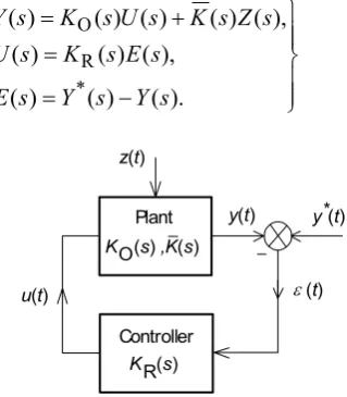
A combination of the case 1 with the case 3 from Sect. 1.3.1 forms a typical and frequently used control system, namely a closed-loop control system with the required output. Such a control is sometimes called a regu-lation. Figure 1.5 presents the simplest block scheme of the closed-loop system with the required output of the plant, containing two basic parts: the control plant CP and the controller C. The small circle symbolizes the comparison of the controlled variable y with its required value y*. It is an example of so called summing junction whose output is the algebraic sum of the inputs. The variable ε(t) = y*– y(t) is called a control error. The controller changes the plant input depending on the control error in order to decrease the value of ε and keep it near to zero in the presence of dis-turbances acting on the plant. For the full automatization of the control it is necessary to apply some additional devices such as a measurement element and an executing organ changing the plant input according to the signals obtained from the controller.
In the example with the furnace, the automatic control may be as fol-lows: the temperature y is measured by an electrical thermometer, the volt-age proportional to y is compared with the voltage proportional to y* and the difference proportional to the control error steers an electrical motor, changing, by means of a transmission, a position of a supplying device and consequently changing the voltage put on the heater. As an effect, the speed of u(t) variations is approximately proportional to the control error, so the approximate control algorithm is the following:
∫
=
t
dt t k t u
0
. ) ( )
Control plant
Controller
ε(t)
z(t)
u(t)
y(t) y*(t)
Fig. 1.5. Basic scheme of closed-loop control system
Depending on y*, we divide the control systems into three kinds: 1. Stabilization systems.
2. Program control systems. 3. Tracking systems.
In the first case y*= const., in the second case the required value changes in time but the function y*(t) is known at the design stage, before starting the control. For example, it can be a desirable program of the temperature changes in the example with the furnace. In the third case the value of y*(t) can be known by measuring only at the moment when it occurs during the control process. For example, y*(t) may denote the position of a moving target tracked by y(t).
1.3.3 Other Cases
Let us mention other divisions or typical cases of control systems: 1. Continuous and discrete control systems.
2. One-dimensional and multi-dimensional systems. 3. Simple and complex control systems.
Ad 1. In a continuous system the inputs of the plant can change at any time and, similarly, the observed variables can be measured at any time. Then in the system description we use the functions of time u(t),y(t), etc. In a dis-crete system (or more precisely speaking – discrete in time), the changes of control decisions and observations may be carried out at certain moments tn. The moments tn are usually equally spaced in time, i.e.
T t
12 1 General Characteristic of Control Systems
called discrete functions of time, that is sequences un,yn etc. where n de-notes the index of a successive period. The computer control systems are of course discrete systems, i.e. the results of observations are introduced and control decisions are brought out for the execution at determined mo-ments. If T is relatively small, then the control may be approximately con-sidered as a continuous one. The continuous control or the discrete control with a small period is possible and sensible for quickly varying processes and disturbances (in particular, in technical plants), but is impossible in the case of a project management or a control of production and economic processes where the control decisions may be made and executed e.g. once a day for an operational management or once a year for a strategic man-agement. A continuous control algorithm determining a dependence of
) (t
u upon w(t) can be presented in a discrete form suitable for the com-puter implementation as a result of so called discretization.
Ad 2. In this book we generally consider multi-dimensional systems, i.e. u, y etc. are vectors. In particular if they are scalars, that is the number of their components is equal to 1 – the system is called one-dimensional. Usually, the multi-dimensional systems in the sense defined above are called multivariable systems. Sometimes the term multi-dimensional is used for systems with variables depending not only on time but also e.g. on a position [76, 77]. The considerations concerning such systems exceed the framework of this book.
1.4 Stages of Control System Design
Quite generally and roughly speaking we can list the following stages in designing of a computer control system:
1. System analysis of the control plant. 2. Plant identification.
3. Elaborating of the control algorithm. 4. Elaborating of the controlling program.
5. Designing of a system executing the controlling program.
The system analysis contains an initial determination of the control goal and possibly subgoals for a complex plant, a choice of the variables char-acterizing the plant, presented in Sect. 1.2, and in the case of a complex plant – a determination of the components (subplants) and their intercon-nections.
The plant identification [14] means an elaboration of the mathematical model of the plant by using the results of observations. It should be a model useful for the determination of the control algorithm so as to achieve the control goal. If it is not possible to obtain a sufficiently accu-rate model, the problem of decision making under uncertainty arises. Usu-ally, the initial control goal should then be reformulated, that is require-ments should be weaker so that they are possible to satisfy with the available knowledge on the plant and (or) on the way of the control.
The elaboration of the control algorithm is a basic task in the whole de-sign process. The control algorithm should be adequate to the control goal and to the precisely described information on the plant, and determined with the application of suitable rational methods, that is methods which are described, investigated and developed in the framework of the control the-ory. The control algorithm is a basis for the elaboration of the controlling computer program and the design of computer system executing this pro-gram. In practice, the individual stages listed above are interconnected in such a sense that the realization of a determined stage requires an initial characterization of the next stages and after the realization of a determined stage a correction of the former stages may be necessary.
14 1 General Characteristic of Control Systems
1.5 Relations Between Control Science and Related Areas
in Science and Technology
After a preliminary characteristic of control problems in Sects. 1.2, 1.3 and 1.4 one can complete the remarks presented in Sect. 1.1 and present shortly relations of control theory with information science and technology, auto-matic control, management, knowledge engineering and systems engineer-ing:
1. The control theory and engineering may be considered as part of the in-formation science and technology, dealing with foundations of computer decision systems design, in particular – with elaboration of decision mak-ing algorithms which may be presented in the form of computer programs and implemented in computer systems. It may be said that in fact the con-trol theory is a decision theory with special emphasis on real-time decision making connected with a certain plant which is a part of an information control system.
2. Because of universal applications regardless of a practical nature of con-trol plants, the concon-trol theory is a part of automatic control and manage-ment considered as scientific disciplines and practical areas. In different practical situations there exists a great variety of specific techniques con-nected with the information acquisition and the execution of decisions. Nevertheless, there are common foundations of computer control systems and decision support systems for management [20] and often the terms control, management and steering are used with similar meaning.
3. The control theory may be also considered as a part of the computer sci-ence and technology because of applications for computer systems, since it deals with methods and algorithms for the control (or management) of computer systems, e.g. the control of a load distribution in a multi-computer system, the admission, congestion and traffic control in com-puter networks, steering a complex computational process by a comcom-puter operating system, the data base management etc. Thus we can speak about a double function of the control theory in the general information science and technology, corresponding to a double role of a computer: a computer as a tool for executing the control decisions and as a subject of such deci-sions.
expert systems [18, 92] in which the generating of control decisions is based on a knowledge representation describing the control plant, or based directly on a knowledge about the control. For the design and realization of the control systems like these, such methods and techniques of the artifi-cial intelligence as the computerization of logical operations, learning al-gorithms, pattern recognition, problem solving based on fuzzy descriptions of the knowledge and the computerization of neuron-like algorithms are applied.
5. The control theory is a part of a general systems theory and engineering which deals with methods and techniques of modelling, identification, analysis, design and control – common for various real systems, and with the application of computers for the execution of the operations listed above.
This repeated role of the control theory and engineering in the areas mentioned here rather than following from its universal character is a con-sequence of interconnections between these areas so that distinguishing be-tween them is not possible and, after all, not useful. In particular, it con-cerns the automatic control and the information science and technology which nowadays may be treated as interconnected parts of one discipline developing on the basis of two fundamental areas: knowledge engineering and systems engineering.
1.6 Character, Scope and Composition of the Book
The control theory may be presented in a very formal manner, typical for so called mathematical control theory, or may be rather oriented to practi-cal applications as a uniform description of problems and methods useful for control systems design. The character of this book is nearer to the latter approach. The book presents a unified, systematic description of control problems and algorithms, ordered with respect to different cases concern-ing the formulations and solutions of decision makconcern-ing (control) problems. The book consists of five informal parts organized as follows.
Part one containing Chaps. 1 and 2 serves as an introduction and pre-sents general characteristic of control problems and basic formal descrip-tions used in the analysis and design of control systems.
Part two comprises three chapters (Chaps. 3, 4 and 5) on basic control problems and algorithms without uncertainty, i.e. based on complete in-formation on the deterministic plants.
16 1 General Characteristic of Control Systems
concerning problem formulations and control algorithm determinations under uncertainty, without obtaining any additional information on the plant during the control.
Part four containing Chaps. 10 and 11 presents two different concepts of using the information obtained in the closed-loop system: to the direct determination of control decisions and to improving of the basic decision algorithm in the adaptation and learning process.
Finally, Part five (Chaps. 12 and 13) is devoted to additional problems of considerable importance, concerning so called intelligent and complex control systems.
To formulate and solve control problems common for different real sys-tems we use formal descriptions usually called mathematical models. Sometimes it is necessary to consider a difference between an exact mathematical description of a real system and its approximate mathemati-cal model. In this chapter we shall present shortly basic descriptions of a variable (or signal), a control plant, a control algorithm (or a controller) and a whole control system. The descriptions of the plant presented in Sects. 2.2−2.4 may be applied to any systems (blocks, elements) with de-termined inputs and outputs.
2.1 Description of a Signal
As it has been already said, the variables in a control system (controlling variable, controlled variable etc.) contain and present some information and that is why they are often called signals. In general, we consider multi-dimensional or multivariable signals, i.e. vectors presented in the form of one-column matrices. A continuous signal
x(t) =
⎥ ⎥ ⎥ ⎥ ⎥
⎦ ⎤
⎢ ⎢ ⎢ ⎢ ⎢
⎣ ⎡
) (
) (
) (
) (
) 2 (
) 1 (
t x
t x
t x
k
is described by functions of time x(i)(t) for individual components. In par-ticular x(t) for k=1 is a one-dimensional signal or a scalar. The term con-tinuous signal does not have to mean that x(i)(t) are continuous functions
18 2 Formal Models of Control Systems
(or Laplace transform) X(s)
=
ˆ
x(t), i.e. the function of a complex vari-able s, which is a result of Laplace transformation of the function x(t):∫
∞− =
0
. ) ( )
(s x t e dt
X st
Of course, the function X(s) is a vector as well, and its components are the operational transforms of the respective components of the vector x. In discrete (more precisely speaking – discrete in time) control systems a discrete signal xn occurs. This is a sequence of the values of x at succes-sive moments (periods, intervals, stages) n=0,1,... . The discrete signal may be obtained by sampling of the continuous signal x(t). Then xn = x(nT) where T is a sampling period. If xn subjects to a linear
transfor-mation, it is convenient to use a discrete operational transform or Z -transform X(z)
=
ˆ
xn , i.e. the function of a complex variable z, which is are-sult of so called Z transformation of the function xn :
. )
(
0
∑
∞ =− =
n
n nz
x z
X
Basic information on the operational transforms are presented in the Ap-pendix.
2.2 Static Plant
A static model of the plant with p inputs and l outputs is a function
y = Φ(u) (2.1)
in a sufficiently long time. For example, it may be a relationship between the amount and parameters of a product obtained at the end of a production cycle and the amount or parameters of a raw material fixed at the begin-ning of the cycle. We used to speak about an inertia-less or memory-less plant if the steady value of the output as a response for the step input set-tles very quickly compared to other time intervals considered in the plant. The function Φ is sometimes called a static characteristic of the plant. Usually, the mathematical model Φ is a result of a simplification and approximation of a reality. If the accuracy of this approximation is suffi-ciently high, we may say that this is a description of the real plant, which means that the value y measured at the output after putting the value u at the input is equal to the value y calculated from the mathematical model after substituting the same value u into Φ. Then we can speak about a mathematical model y=Φ(u) differing from the exact description Φ. Such a distinction has an essential role in an identification problem. Usu-ally, instead of saying a plant described by a model Φ, we say shortly a plantΦ, that is a distinction plant – model is replaced by a distinction real plant – plant. In particular, the term static model of a real plant is replaced by static plant. Similar remarks concern dynamical plants, other blocks in a system and a system as a whole.
For the linear plant the relationship (2.1) takes the form
y = Au + b
where A∈ Rl×p, i.e. A is a matrix with l rows and p columns or is l×p ma-trix; b is one-column matrix l×1. Changing the variables
b y
y= −
we obtain the relationship without a free term. As a rule, the variables in a control system denote increments of real variables from a fixed reference
point. The location of the origin in this point means that Φ(0)=0 where 0 denotes the vector with zero components. The model (2.1) can be pre-sented as a set of separate relationships for the individual output variables:
y(j)=Φj(u), j = 1, 2, ..., l.
2.3 Continuous Dynamical Plant
time-20 2 Formal Models of Control Systems
continuous manner, that is systems where the control variables can change at any time and, similarly, the observed variables can be measured at any time. Thus a dynamic model will involve relations between the time func-tions describing changes of plant variables. These relafunc-tionships will most often take the form of differential equations for the plants controlled con-tinuously, or difference equations for the plants controlled discretely. Other forms of relations between the time functions characterizing a con-trol plant may also occur.
There are three basic kinds of descriptions of the properties of a dy-namic system with an input and an output (control plant in our case): 1. State vector description.
2. “Input-output” description by means of a differential or difference equa-tion.
3. Operational form of the “input-output” description.
The last two kinds of description represent, in different ways, direct rela-tions between the plant input and output signals.
2.3.1 State Vector Description
To represent relations between time-varying plant variables, we select a sufficient set of variables x(1)(t), x(2)(t), ..., x(k)(t) and set up a mathemati-cal model in the form of a system of first order differential equations:
⎪ ⎪ ⎭ ⎪ ⎪ ⎬ ⎫ = = = ). ,..., , ; ,..., , ( ... ... ... ... ... ... ... ... ), ,..., , ; ,..., , ( ), ,..., , ; ,..., , ( ) ( ) 2 ( ) 1 ( ) ( ) 2 ( ) 1 ( ) ( ) ( ) 2 ( ) 1 ( ) ( ) 2 ( ) 1 ( 2 ) 2 ( ) ( ) 2 ( ) 1 ( ) ( ) 2 ( ) 1 ( 1 ) 1 ( p k k k p k p k u u u x x x f x u u u x x x f x u u u x x x f x (2.2)
The variables u(1), u(2), ..., u(p) denote input signals (control signals, in par-ticular). Thus we consider a multi-input plant with p inputs. If we are in-terested in the plant output variables, then the relations between the output signals y(1), y(2), ..., y(l) (l-output plant), x(1), x(2), ..., x(k) and u(1), u(2), ..., u(p), have also to be determined:
In practice, because of the inertia inherent in the plant, the signals u(1), u(2), ..., u(p) usually do not appear in the equation (2.3). The equations (2.2) and (2.3) can be written in a briefer form using vector notation (with u already eliminated from the equation (2.3)):
⎭ ⎬ ⎫ = = ) ( ), , ( x y u x f x η (2.4) where
x =
⎥ ⎥ ⎥ ⎥ ⎥ ⎦ ⎤ ⎢ ⎢ ⎢ ⎢ ⎢ ⎣ ⎡ ) ( ) 2 ( ) 1 ( k x x x
, u =
⎥ ⎥ ⎥ ⎥ ⎥ ⎦ ⎤ ⎢ ⎢ ⎢ ⎢ ⎢ ⎣ ⎡ ) ( ) 2 ( ) 1 ( p u u u
, y =
⎥ ⎥ ⎥ ⎥ ⎥ ⎦ ⎤ ⎢ ⎢ ⎢ ⎢ ⎢ ⎣ ⎡ ) ( ) 2 ( ) 1 ( l y y y .
The sets of functions f1, f2, ..., fk and η1, η2, ..., ηl are now represented by f and η. The function f assigns a k-dimensional vector to an ordered pair of k- and p-dimensional vectors. The function η assigns an l-dimensional vec-tor to a k-dimensional one. If u(t) = 0 for t ≥ 0 (or, in general, u(t) = const), then the first of the equations (2.4) describes a free process
x=f(x) (2.5)
and, for a given initial condition x0 = x(0), the solution of the equation
(2.5) defines the variable x(t)
x(t) = Φ (x0, t).
Under the well-known assumptions, knowledge of the function f and of the value x(t1) uniquely determines x(t2) for any t2>t1:
x(t2) = Φ[x(t1), t1, t2].
22 2 Formal Models of Control Systems
The choice of state variables for a given plant can be done in infinitely many ways. If x is a state vector of a certain plant, then the k-dimensional vector
v = g(x) (2.6)
where g is a one-to-one mapping, is also a state vector of this plant. The transformation (2.6) may, for example, be linear
v = Px
where P is a non-singular matrix (i.e. detP≠0). Substituting )
(
1 v
g
x= −
into the equations (2.4), we obtain the new equations
⎭ ⎬ ⎫ =
= ). (
), , (
v y
u v f v
η
(2.7)
The descriptions (2.4) and (2.7) are said to be equivalent. Thus different choices of the state vector yield equivalent descriptions of the same plant. In particular, if l = k and η in the equation (2.4) is a one-to-one mapping, then y is a state vector of the plant. We say then that the plant is measur-able, which means that knowledge of the output y at a time t uniquely de-termines the state of the plant at this time. Since we always assume that the output signals y can be measured, it is therefore implied that, in the case of a measurable plant, all the state variables can be measured at any time t. In particular, for a linear plant, under the assumption that f(0,0)= 0
and η(0)= 0 , the description (2.4) becomes
⎭ ⎬ ⎫ =
+
= ,
Cx y
Bu Ax x
(2.8)
where A is a k×k matrix, B is a k×p matrix and C is a l×k matrix. In the case of a single-input and single-output plant (p = l = 1) we write the equations (2.8) in the form
⎭ ⎬ ⎫ =
+
= ,
Tx
c y
bu Ax x
(2.9)
⎭ ⎬ ⎫ =
=
). , (
), , , (
t x y
t u x f x
η
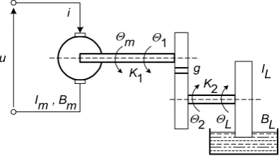
Example 2.1. Let us consider an electromechanical plant consisting of a D.C. electrical motor driving, by means of a transmission, a load contain-ing viscous drag and inertia (Fig. 2.1).
u
i
Im , Bm
IL
BL
g
K2
Θ2 ΘL Θm Θ1
[image:31.439.124.322.159.271.2]K1
Fig. 2.1. Example of electromechanical plant
The dynamic properties of the system can be described by the equations:
u = L dt di
+ r i + Kb dt dΘm
,
M = Kb⋅i,
M = Im
2 2
dt
d Θm
+ Bm dt dΘm
+ K1(Θm – Θ1),
Θ2 =
g 1
Θ1,
gK1(Θ1 – Θm) = K2(ΘL – Θ2),
IL 2
2
dt
d ΘL
+ BL
dt dΘL
+ K2(ΘL – Θ2) = 0
where u is the supply voltage, i – the current, Θm – the angular position of
24 2 Formal Models of Control Systems
the moments of inertia of the rotor and load, respectively, Bm and BL – the friction coefficients of the rotor and load; K1 , K2 , L, r, Kb – the other
pa-rameters, g – the transmission ratio. On introducing five state variables:
x(1) = i, x(2) = Θm, x(3) = Θm, x(4) = ΘL, x(5) = ΘL
the plant equations, after some transformation, can be reduced to the form
) 1 (
x = –
L r
x(1) – L Kb
x(3) + L 1 u, ) 2 (
x = x(3),
) 3 (
x =
m b
I K
x(1) + αx(2) –
m m
I B
x(3) + β x(4),
) 4 (
x = x(5),
) 5 (
x = γ x(2) + δx(4) –
L L I B x(5) where
α =
)
( 2 1 2
2 1 K K g I K K m +
− , β =
)
( 2 1 2
2 1 K K g I K gK m + ,
γ =
)
( 2 1 2
2 1 K K g I K gK L +
, δ =
)
( 2 1 2
2 1 2 K K g I K K g L + − .
□
2.3.2 “Input-output” Description by Means of Differential Equation
The relationship between the input vector u(t) and the output vector y(t) can be described by means of a differential equation
F1( , ,..., , )
1 1 y dt dy dt y d dt y d m m m m − −
= F2( , ,..., , )
1 1 u dt du dt u d dt u d v v v v − − .
m m
dt y d
+ Am–1 1 1
− −
m m
dt y d
+ ... + A1 dt dy
+ A0 y
= Bv
v v
dt u d
+ ... + B1 dt du
+ B0 u (2.10)
where Ai (i = 0, 1, ..., m – 1) are l×l matrices, Bj (j = 0, 1, ..., v) are l×p
ma-trices.
In particular, for single-input and single-output plant (p = l =1)
y(m) + am–1 y(m–1) + ... + a1y + a0y = bvu(v) + ... + b1u + b0u.
In a non-stationary plant at least some of the coefficients a and (or) b are functions of t.
2.3.3 Operational Form of “Input-output” Description
The relation between the input and the output plant signals can be de-scribed by means of an operator Φ which transforms the function u(t) into the function y(t):
y(t) = Φ[u(t)]. (2.11)
For example, in the case of a one-dimensional linear plant (p = l = 1) with zero initial conditions, the formula (2.11) is
y(t) =
∫
t
i t u d
k
0
) ( ) ,
( τ τ τ (2.12)
where ki(t, τ) is the weighting function (time characteristic) of the plant.
For linear plants with constant parameters, the type of models consid-ered includes description by means of operational transmittance. Applying an operational transformation to the both sides of the equation (2.10), un-der zero initial conditions, we obtain
(Ism +
∑
− =1
0 m
i i is
A )Y(s) = (
∑
=v
j j js
B
0
)U(s) (2.13)
where I is the unit matrix, and Y(s) and U(s) denote Laplace transforms of the vectors y(t) and u(t), respectively. From the equation (2.13) we have
26 2 Formal Models of Control Systems
where
K(s) = (Ism +
∑
−=
1
0 m
i i is
A )–1
∑
=
v
j j js
B
0
.
The matrix K(s) is called a matrix operational transmittance (or matrix transfer function) of the plant. Its elements are rational functions of s. In the case of one-dimensional plant K(s) is itself such a function, i.e.
K(s) = ) (
) (
s U
s Y
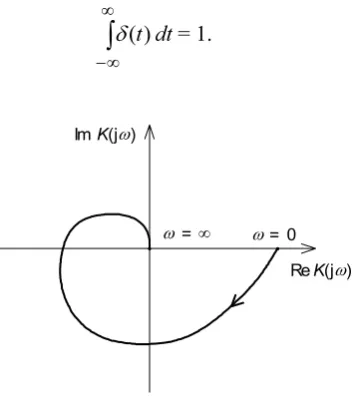
where Y(s) and U(s) are polynomials. In real systems the degree of the numerator is not greater than the degree of the denominator. This is the condition of so called physical existence (or a physical realization) of the transmittance. The transmittance is related to equivalent descriptions of the plant, namely to the gain-phase (or amplitude-phase) characteristics and time characteristics (unit-step response and impulse response).
A gain-phase characteristic or a frequency transmittance is defined as K(jω) for 0 ≤ω<∞. The graphical representation of this function on K(s) plane is sometimes called a gain-phase plot or Nyquist plot. If u(t) = A sinωt then in the steady state the output signal y(t) is sinusoidal as well: y(t) = B sin(ωt+ϕ) . It is easy to show that
|K(jω)| = A B
, arg K(jω) = ϕ.
For example, the frequency transmittance K(jω) for
K(s) =
) 1 )( 1 )( 1
(sT1+ sT2+ sT3+ k
is illustrated in Fig. 2.2. Let
u(t) = ⎩ ⎨ ⎧
< ≥
. 0 for 0
0 for 1
t t
Such a function is called a unit step and is denoted by 1(t). The response of
∫
∞∞ −
dt t) (
δ = 1.
ImK(jω)
[image:35.439.127.305.68.270.2]ReK(jω) ω =∞ ω = 0
Fig. 2.2. Example of frequency transmittance
The response of the plant y(t) ∆=ki(t) for the input u(t) = δ(t) is called an impulse response. It is easy to prove that the transmittance K(s) is Laplace
transform of the function ki(t) and ki(t) = k(t). For the linear stationary plant, the relationship (2.12) takes the form
y(t) =
∫
−t
i t u d
k
0
) ( )
( τ τ τ .
For example, the plant described by the equation
Ty(t) + y(t) = k u(t)
has the transmittance
K(s) = 1 + Ts
k ,
the unit-step response
k(t) = k(1 – T t
e− )
28 2 Formal Models of Control Systems
ki(t) =
T
k Tt
e− .
Such a plant is called a first order inert element (or an element with iner-tia). It is worth recalling that the descriptions presented here are used not only for plants but in general – for any dynamical elements or blocks with determined inputs and outputs. Basic elements are presented in Table 2.1.
Table 2.1
Name of the element Transmittance
Inertia-less element K(s) = k
First order inert element K(s) =
1
+
sT k
Integrating element with first order inertia K(s) =
) 1 (sT+ s
k
Differentiating element with first order inertia K(s) =
1
+
sT sk
Oscillation element K(s) =s + αs+β k
2
2 ,
β>α2
Complex blocks may be considered as systems composed of basic blocks. Figure 2.3 presents a cascade connection and a parallel connection of two blocks with the transmittance K1(s) and K2(s).
K1 K2 y
K2
K1
u
y1
u
u
u y2
y=y1+y2
+ +
a) b)
Fig. 2.3. a) Series connection, b) parallel connection
For multi-dimensional case, in the case of the cascade connection the number of outputs of the block K1 must be equal to the number of inputs
must have the same number of inputs and the same number of outputs. For the cascade connection
Y(s)=K2(s)K1(s)U(s).
For the parallel connection
Y(s)=[K1(s)+K2(s)]U(s).
More details concerning the descriptions of linear dynamical blocks and their examples may be found in [14, 71, 76, 88].
2.4 Discrete Dynamical Plant
The descriptions of discrete dynamical plants are analogous to the corre-sponding descriptions for continuous plants presented in Sect. 2.3. The state vector description has now the form of a set of first-order difference equations, which in vector notation is written as follows:
⎭ ⎬ ⎫ =
= +
. ) (
), , (
1
n n
n n n
x y
u x f x
η
The “input-output” description by means of the difference equation is now:
F1(yn+m, yn+m−1,...,yn)=F2(yn+v, un+v−1,...,un).
In particular, the linear model has the form of the linear difference equa-tion
yn+m+Am−1yn+m−1 +...+A1yn+1 +A0yn
= Bvun+v+Bv−1un+v−1 +...+B1un+1 +B0un,
and the operational description is as follows:
Y(z)=K(z)U(z)
where K(z) denotes the discrete operational transmittance:
K(z) = (Izm +
∑
−∑
= =
−
1
1 1
1( )
)
m
i
v
j j j i
iz B z
A .
30 2 Formal Models of Control Systems
The functions Y(z) and U(z) denote here the discrete operational trans-forms (Z-transforms) of the respective discrete signals yn and un. The
K(ejω) for −π<ω<π is called a discrete frequency transmittance ( dis-crete gain-phase characteristic).
We shall now present the description of a continuous plant being con-trolled and observed in a discrete way. Consequently, we have a discrete plant whose output yn is a result of sampling of the continuous plant out-put, i.e. yn=y(nT) where T is the control and observation period. The input
of the continuous plant v(t) is formed by a sequence of decisions un deter-mined by a discrete controller and treated as the input of the discrete plant. It is a typical situation in the case of a computer control of the continuous plant. In the simplest case one assumes that v(t)=un for nT≤t<(n+1)T. Such a signal for one-dimensional input can be presented as an effect of putting a sequence of Dirac impulses unδ(t−nT) at so called zero-order holdEO (see Fig. 2.4) with the transmittance
KE(s)= s e−sT − 1
where e−sT denotes a delay equal to T. It may be shown that the
transmit-tance of the discrete plant with the input un and the output yn is equal to the Z-transform of the function ki(nT) where ki(t) denotes the impulse response of the element with transmittance KE(s)KO(s), and KO(s) denotes the transmittance of the continuous plant. It is easy to note that
ki(t)=ki(t)−ki(t−T)1(t–T) (2.14) where ki(t) is the impulse response of the element with the transmittance
) ( 1
O s
K
s .
yn
un v(t) y(t)
EO KO
Fig. 2.4. Discrete plant with zero-order hold
1 )
(
0 O
+ =
sT k s
K .
It is easy to find
) 1
( )
( 0
0 T
t
i t kt kT e
k
− − −
= .
After substituting ki(t) into (2.14), putting t=nT and applying Z-transformation, we obtain
D z D z
T T D T z D T T k z K
+ + −
+ − + − − =
) 1 (
) ( )]
1 ( [ ) (
2
0 0 0
where exp( )
0
T T
D= − .
□
2.5 Control Algorithm
In Chap. 1 we have introduced a term controlling device or controller as an executor of the control algorithm. Hence the control algorithm may be considered as a description (mathematical model) of the controller. Since the descriptions of the plant presented in the previous sections can be ap-plied to any elements or parts with a determined input and output, then they can be used as the basic forms of a control algorithm in these cases when it may be presented in an analytical form, i.e. as a mathematical for-mula. We shall often use the term controller in the place of a control algo-rithm (and vice versa) as well as the term plant in the place of a model of the plant. Let us denote by w the input variable of the control algorithm (see similar notation concerning the controller in Sect. 1.2). Then a static control algorithm has the form
u = Ψ(w)
and a continuous dynamical control algorithm presented by means of the state vector xR(t) is described by a set of equations
)] ( ), ( [ )
( R R
R t f x t w t
x = ,
u(t) = ηR[xR(t)].
32 2 Formal Models of Control Systems
equation or descriptions in an operational form – analogous to those pre-sented for a plant. For example, in technical control systems one often uses the one-dimensional controller described by the equation
) ( ) ( ) ( )
(t k1 t k2 t k3 t
u = ε + ε + ε
or
∫
++ =
t
t k dt t k t k t u
0
3 2
1 ( ) ( ) ( )
)
( ε ε ε
where ε(t) denotes the control error. This is so called PID controller, or proportional-integrating-differentiating controller. Its transmittance
s k s k k s E
s U s
KR 1 2 3
) (
) ( )
( = = + +
where E(s) is the Laplace transform of the function ε(t).
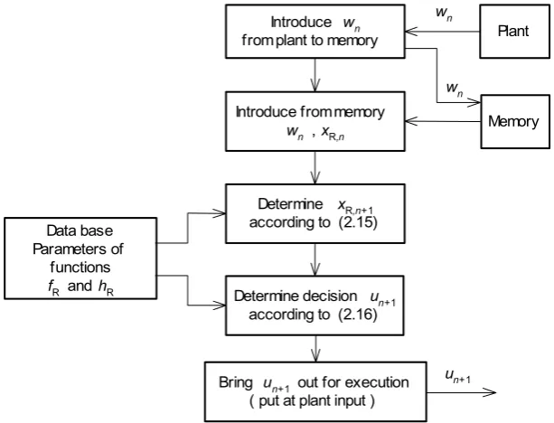
Similarly, the forms of a discrete dynamical control algorithm are such as the descriptions of a discrete plant presented in Sect. 2.4. This is a con-trol algorithm with a memory, i.e. in order to determine the decision un it is necessary to remember the former decisions and the values w. The de-scription of the algorithm is used as a basis for elaborating the correspond-ing program for the computer realization of the algorithm in a computer control system. One may say that it is an initial description of the control program. The block scheme of the algorithm written in the form
xR,n+1 = fR(xR,n, wn ) (2.15)
un= ηR(xRn) (2.16)
is presented in Fig. 2.5. The controlling computer determines the decisions un in a real-time, in successive periods (intervals) which should be
suffi-ciently long to enable the computer to calculate the decision un in one in-terval. It determines the requirements concerning the execution time of the control program. The description of the control algorithm in the form of the difference equation is as follows:
un+m + am–1un+m–1+ ... + a1un+1 + a0un
= bm–1wn+m–1 + ... + b1wn+1 + b0wn.
un = –am–1un–1 – ... – a1un–m+1 – a0un–m + bm–1 wn–1
+ ... + b1wn–m–1– b0 wn–m.
This is the direct prescription for finding un by using the former values u and w, and the coefficients a and b placed in the data base. The number m determines the required length of the memory.
Introduce wn
from plant to memory
Introduce from memory
wn ,xR,n
Determine xR,n+1
according to (2.15)
Determine decision un+1
according to (2.16)
Bring un+1 out for execution ( put at plant input )
Plant
Memory
Data base Parameters of
functions
fR andhR
wn
wn
[image:41.439.68.375.165.399.2]un+1
Fig. 2.5. Basic block scheme of control algorithm
2.6 Introduction to Control System Analysis
The description of the control system consists of formal models of the parts in the system and the description of the structure, that is interconnec-tions between the parts. For example, the description of the closed-loop discrete control system by means of the state vector is the following
⎪⎭ ⎪ ⎬ ⎫ =
= +
), (
), , , (
, O O
, O O 1 , O
n n
n n n n
x y
z u x f x
34 2 Formal Models of Control Systems
⎪⎭ ⎪ ⎬ ⎫ =
= +
) (
), , , (
, R R
* R,
R 1 R,
n n
n n n n
x u
y y x f x
η (2.18)
where xO,n is the state vector of the plant, xR,n is the state vector of the
controller, zn is the vector of external disturbances acting on the plant, y*n is the varying required value. Thus, in the system two basic parts are de-termined: the plant (2.17) and the controller (2.18). If it is the control error
εn= y*n– yn which is put at the input of the plant, then the first equation in
(2.18) takes the form
xR,n+1 = fR(xR,n , εn).
The control system under consideration may be treated as one dynamical
block whose state is c =nT [xOT,n,xRT,n] and whose inputs are the
distur-bances zn and y*n. This block is described by the equations
⎪⎭ ⎪ ⎬ ⎫ =
= +
) (
), , , (
O, O
* 1
n n
n n n n
x y
y z c f c
η (2.19)
if we consider yn as the output of the system as a whole. The first equation in (2.19) may be obtained via the elimination of un and yn from the sets (2.17) and (2.18), i.e. by substituting un=ηR(xR,n) into the first equation in (2.17) and yn = ηO(xO,n) into the first equation in (2.18). The description of the continuous control system by means of the state vector is analogous to that presented above for the discrete system.
The description of the control system forms a basis for its analysis. We may consider a qualitative analysis consisting in the investigation of some properties of the system (e.g. stability analysis) or a quantitative analysis consisting in the determination of a response of the system for a deter-mined input and the determination of a performance (quality) index. For example, the analysis of the dynamical control system may consist in find-ing the transit response yn for the given initial state c0 and the given