OXFORD UNIVERSITY CENTRE FOR EDUCATIONAL ASSESSMENT
Marker effects and examination reliability
A comparative exploration from the perspectives of
generalizability theory, Rasch modelling and multilevel
modelling
Jo-Anne Baird, Malcolm Hayes, Rod Johnson, Sandra Johnson & Iasonas Lamprianou
January 2013
Ofqual/13/5261
Content
1 EXECUTIVE SUMMARY ... I 1.1 RESEARCH CONTEXT, AIMS AND OBJECTIVES ... I
1.2 THE DATASETS ... I
1.3 THE THREE ANALYSIS TECHNIQUES AND THEIR FINDINGS ... II
1.4 DATA ISSUES ... IV
1.5 CONCLUSIONS ... IV
1.6 ACKNOWLEDGEMENTS ... V
2 INTRODUCTION ... 1
2.1 PROJECT OVERVIEW ... 1
2.2 PREVIOUS RESEARCH ON RATERS AND THEIR EFFECTS... 2
2.2.1 Rater severity ... 2
2.2.2 Training group effects ... 3
2.2.3 Monitoring system effects ... 4
2.3 MARKER-FOCUSED RESEARCH WITHIN OFQUAL’S RELIABILITY PROGRAMME ... 5
2.4 RESEARCH QUESTIONS ... 7
3 THE DATASETS ... 9
3.1 THE COMPONENT PAPERS ... 9
3.2 MARKER STANDARDISATION ... 10
3.2.1 Division of responsibilities ... 10
3.2.2 Marker training ... 10
3.3 THE OPERATIONAL MARKING PROCESS... 11
3.4 THE RESULTING MARK DISTRIBUTIONS ... 13
4 GENERALIZABILITY THEORY ... 16
4.1 OVERVIEW OF G-THEORY ... 16
4.2 VARIANCE DECOMPOSITION ... 18
4.3 FROM SCRIPT MARKING TO CLIP MARKING ... 22
4.4 GEOGRAPHY G-STUDY ANALYSES AND FINDINGS ... 24
4.4.1 Marker effects study for geography (operational data) ... 25
4.4.2 Seeded clip analyses for geography ... 29
4.5 PSYCHOLOGY G-STUDY ANALYSES AND FINDINGS ... 32
4.5.1 Marker effects study for psychology (operational data) ... 32
4.5.2 Seeded clip analyses for psychology ... 35
4.6 DATA LIMITATIONS ... 37
5 RASCH MODELLING ... 39
5.1 THE MANY-FACETS RASCH MODEL (MFRM) ... 40
5.2 ASSUMPTIONS OF THE MODEL ... 41
5.3 MFRMANALYSES ... 42
5.4 RASCH FINDINGS – PSYCHOLOGY ... 45
5.5 RASCH FINDINGS – GEOGRAPHY ... 50
6 MULTILEVEL MODELLING ... 52
ii
6.3 MULTILEVEL MODELLING FINDINGS FOR GEOGRAPHY ... 56
6.4 MULTILEVEL MODELLING FINDINGS FOR PSYCHOLOGY ... 60
7 REFLECTIONS AND CONCLUSIONS ... 63
7.1 THE IMPACT OF INTER-RATER RELIABILITY ... 63
7.2 STABILITY OF RATER EFFECTS: INTRA-RATER RELIABILITY ... 63
7.3 QUESTION EFFECTS ... 64
7.4 TRAINING GROUP EFFECTS ... 64
7.5 THE THREE APPROACHES TO RATER EFFECT INVESTIGATION ... 64
7.6 THE CRAFT OF ANALYSIS ... 67
7.7 LIMITATIONS OF THE STUDY ... 67
7.8 IMPLICATIONS FOR FUTURE QUALITY MONITORING PROCESSES ... 68
8 REFERENCES ... 69
Table 1 Monitoring systems used in the Baird, Leckie and Meadows study ... 5
Table 2 Monitoring systems used in the current study ... 5
Table 3 Clip statistics for geography ... 13
Table 4 Clip statistics for psychology ... 13
Table 5 Candidate numbers for the geography unit paper ... 25
Table 6 Variance breakdown for the single-marked operational datasets for geography ... 26
Table 7 Predicted precision of markers’ mean clip scores in geography ... 28
Table 8 Composite score reliability for geography (relative generalizability coefficients) ... 29
Table 9 Clip-level data availability for geography in 2011 ... 30
Table 10 Generalizability analyses of seeded clip data for geography in 2011 ... 31
Table 11 Estimated candidate reliability for single-marked geography items in 2011 ... 31
Table 12 Variance breakdown for the single-marked operational datasets for psychology ... 33
Table 13 Predicted precision of markers’ mean clip scores in psychology ... 34
Table 14 Composite score reliability for psychology (relative generalizability coefficients) ... 35
Table 15 Seeded clip statistics for psychology in 2011 ... 36
Table 16 Generalizability analyses of seeded clip data for psychology in 2011 ... 37
Table 17 Estimated candidate reliability for single-marked psychology items in 2011 ... 37
Table 18 Operational subsets for the psychology data in the Rasch analyses ... 45
Table 19 Indices of rater effects for the three psychology datasets ... 48
Table 20 Correlation between rater measures for different years ... 49
Table 21 Indices of rater effects for the three geography datasets ... 51
Table 22 Multilevel model for geography multiply-marked data (2009-11) ... 57
Table 23 Multilevel model for psychology multiply-marked data (2009-11) ... 60
Figure 1 The mark distributions for the geography unit papers 2009-2011... 14
Figure 2 The mark distributions for the psychology unit papers 2009-2011 ... 15
Figure 3 The c x q x m design ... 19
Figure 5 The c:(moq) design ... 23
Figure 6 Section score distributions for psychology in 2011 ... 35
Figure 7 Histograms - Infit Mean Square fit for psychology candidates (all 3 years) ... 47
Figure 8 Distribution of rater effects for the three psychology datasets ... 49
Figure 9 Correlation of rater measures across years (psychology data) ... 50
Figure 10 Classification structure ... 53
Figure 11 Rater effects for the seeded (top) and backread data (bottom) – geography ... 59
Figure 12 Plot of rater effects for each monitoring system - geography ... 59
Figure 13 Rater effects for the seeded (top) and backread data (bottom) - psychology ... 62
Marker effects and examination reliability
1
Executive Summary
1.1 Research context, aims and objectives
This collaborative research project was a comparative study of the contributions that three different analysis methodologies could make to the exploration of rater effects on examination reliability. The analysis techniques in question were Generalizability Theory (G-theory), Item Response Theory (IRT) – in particular the Many-Facets Partial Credit Rasch Model (MFRM), and Multilevel Modelling (MLM). The examination datasets supplied for use in the project were AS component papers in two large-entry subjects – geography and psychology – for the three consecutive years 2009, 2010 and 2011.
Rater effects can be grouped into two broad types: inter-rater effects and intra-rater effects (also known as interaction effects). Arguably the best known, and certainly the most researched, inter-rater effect is that of between-rater difference in overall rating standards, i.e. differences in severity/leniency. Intra-rater effects, which have been less well covered in the literature, take many different forms, but are all examples of departures from the general pattern of inter-rater difference in severity/leniency. Rater-candidate interaction effects, question interaction effects, and rater-occasion interaction effects (‘marker-drift’ if the pattern of differences is clearly a trend over time) are all evidence of intra-rater effects.
This project set out to explore both inter-rater effects and intra-rater effects. Given the findings from previous research, we initially set out to investigate
the impact of inter-rater reliability the stability of rater severity effects question effects
the effect of training group on marker behaviour
the effect of training approach (face-to-face versus on-line standardisation). In the event, in only one year (2009) for one subject (psychology) was marker
standardisation conducted face-to-face, so that the last research objective in the list was intractable with the available data.
1.2 The datasets
periodic quality check took place. In one type, ‘backreading’, marked clips were diverted by the automated delivery system from time to time to be re-marked by the marker’s team leader (now acting as marking supervisor). The supervisor re-marked the clip, but with knowledge of the original marker’s mark. Where there was a difference of opinion the supervisor’s mark overrode the original mark as a contribution to the candidate’s final composite score for the paper. In the other type of quality check a set of clips that had been pre-marked by the chief examiner at the time of marker standardisation were ‘seeded’ to markers in their clip allocations. The markers marked these clips without knowledge of their status or of their pre-assigned marks.
As a result, each annual subject dataset comprised three types of record, or three data subsets, reflecting the three different processes: the operational marking, the backread quality check marking, and the seeded clip quality check marking. The majority of records were ‘operational’, which means that they were the result of one marker marking one clip.
1.3 The three analysis techniques and their findings
G-theory, Rasch modelling and multilevel modelling each in principle have something to offer rater effects research. The first, G-theory, is essentially a sampling approach to reliability investigation, generalising sample-based findings to a given population or universe. It focuses on variance analysis, and makes no distributional assumptions. G-theory analysis is most effective when a given dataset allows the potential to explore not only main effects (e.g. in this context of markers, questions, teams) but also, critically, those interaction effects that contribute to measurement unreliability (marker-question interaction, marker-occasion interaction, etc.).
For Item Response Theory (IRT) the model of choice for data analysis was the Many-Facets Partial Credit Rasch Model (MFRM). Like all IRT modelling techniques, MFRM is in essence a scaling technique. The power of the technique is that, provided some quite strong assumptions are met, in particular that there are minimal interaction effects evident in the data, markers, questions and candidates can be located in terms of relative severity, difficulty and ability, respectively, on the same underlying logit scale.
Multilevel modelling is an explanatory approach, which, like G-theory, quantifies the relative contributions to variance of the factors identified in the analysis model. An essential assumption underpinning a multilevel analysis is that all variables are normally distributed. Multilevel models can be conceived of as an extension to
Marker effects and examination reliability
being nested within examiners. Multilevel modelling has expanded our capacity to model complex data structures.
The unit of analysis in every case was a candidate mark on a question or part-question, i.e. a clip score. In each subject the three annual datasets were separately analysed using G-theory and MFRM to investigate rater effects and measurement reliability. Both techniques were used on the single-marked operational datasets; follow-on MFRM repeat analyses combined seeded clip data with single-marked operational data, whereas further G-theory analyses looked at seeded clip data alone. Multilevel modelling analyses, on the other hand, combined all backread and seeded clip data records over all three years across both subjects, and excluded the single-marked operational data.
It was not possible to carry out a ‘team effect’ analysis using MFRM, because of disjoined subsets (since individual markers were naturally assigned to one team only, team
membership was mutually exclusive). G-study analyses were able to explore team effects within years, and found no evidence of these. Team effects were analysed in the multilevel model for geography and were found to be very small. Caveats have to be placed upon the multilevel findings regarding teams, however, as there were fewer teams (15) than necessary to safely conduct these analyses.
Stability of rater effects was investigated in different ways using the three methodologies. In MFRM, the rater effects were found to have non-significant correlations between years for the psychology data. Generalizability analyses
investigated marker drift within each examination series and found no evidence that marker behaviour changed over the period of operational marking. The multilevel models were set up to investigate stability of rater effects across marker monitoring systems and found that rater effects correlated moderately across the backread and seeded systems. Across years, moderate correlations of rater effects were found in geography, but there were non-significant correlations in psychology (in keeping with the MFRM finding).
As far as marker contributions to clip score variance is concerned, both the G-theory analyses and the multilevel analyses found inter-rater effects to be modest in
the effect was smaller for the 2011 psychology dataset. However, a particular feature to note that might create uncertainty about the validity of these findings is that there was an unusually high proportion of candidate misfit, both in psychology and in geography, meaning that the Rasch model did not fit the data well. This is probably explained by the presence of the kinds of interaction effects noted in the G-theory analyses, given that in the MFRM these are assumed in principle to be absent (the Rasch model can
accommodate interaction effects to some extent, but only up to a point).
1.4 Data issues
The single-marked operational data were useful for investigating rater effects of different kinds. But they could never provide an estimate of the reliability with which examination candidates had actually been measured by the component paper
investigated. The backread data could not do this either, given that the (only) two markers who marked each clip were not marking independently (the backreading supervisor was aware of the mark already assigned by the regular marker). The only data with any possibility of offering this option would have been the seeded clip data, given that most or all of the regular markers had independently marked each seeded clip without knowledge of the pre-assigned ‘expert’ mark.
The seeded clip exercise, though, had not been designed to serve this purpose on these occasions. The samples of seed clips were very small and uneven in size. Moreover, they had not been randomly selected to represent either the total entry for the subject
concerned in the year in question, nor were they randomly selected to represent some identifiable subset – such as clips within five marks of a grade boundary. This meant that any analysis based on seeded clip data would probably not be well-based
(estimation errors would be high) and generalisation would be limited in value. The fact that from one part-question to another the seed clips samples were from different candidates reduced even further the possibility of estimating measurement reliability at component level. This is an area that warrants consideration for the future, since the seed clip strategy could without too much additional cost and effort be re-designed and expanded to serve both the current operational quality check needs and the need to provide component-level reliability statistics. The project team has experience of analysis of these kinds of data from a range of examinations and electronic systems and the issues we raise here are general.
1.5 Conclusions
Marker effects and examination reliability
terms of their estimated overall severity/leniency, found large marker differences (though model fit was poor). Neither did the G-theory analyses reveal any evidence of training team effects. Measures of marker performance were found to be stable within an examination series in the generalizability analyses, but the MFRM and the multilevel analyses showed these to be moderately stable at best between years and between the two monitoring systems (backread and seeding). However, since rater effects were small, we would not necessarily expect high correlations.
We aimed to tackle a number of research questions using three advanced statistical methods, to compare them and to do all of this using operational datasets. In the timescale of this study, the project was ambitious and difficult. It is clear that much more could be done to compare the data using these techniques, as the methods offer the capacity to analyse the data in a range of other ways. As such, some of our findings are not relative limitations of the methods per se, but artefacts of the ways in which we have currently analysed the data for the purposes of this report. In a short project it is not possible to explore all possibilities, but this report nevertheless represents an important advance upon the previous literature and a basis upon which future research can build.
1.6 Acknowledgements
This research was commissioned by Ofqual. We would also like to acknowledge Pearson for providing data for analysis. Rose Clesham and Jeremy Pritchard of Edexcel also assisted the research by clarifying our interpretations of the data. Jo Hazell
administered the project and Yasmine El Masri assisted with the finalisation of the report.
2
Introduction
2.1 Project overview
In the eyes of the public, rater reliability is paramount for English public examinations (Ipsos MORI, 2009, p.21). Public examinations need to offer a common yardstick, so inter-rater reliability assumes a great deal of significance in systems where external examinations are used for high stakes assessments. Kingsbury (1922) categorised the effects that examiners could have upon scores in terms of
severity, halo and
central tendency effects.
Severity effects arise when examiners differ markedly in their leniency/severity, halo effects involve a positive biasing effect of part of a candidate’s performance upon the assessment of other parts, and central tendency effects relate to the extent to which examiners use the entire range of the mark scale. These are all systematic effects that can readily be observed in the resulting marking data. In addition to these are
unsystematic effects that can be grouped under the term ‘marker inconsistency’. Examples are particular markers scoring particular scripts more or less severely than normal, and markers scoring erratically over a period of time as opposed to showing consistent trends towards greater or lesser severity. These various aspects of marker behaviour are widely referred to as ‘rater effects’ in the literature and we use this term here.
Information about rater reliability for a given set of scores produced under particular administration conditions for specific assessments is useful for quality assurance and quality control. To improve the quality of rating, assessment organisations can address systemic aspects of their processes, such as marker training. Additionally, the
performance of individual examiners is monitored and controlled. With the
introduction of on-screen marking, the capacity for measuring and assuring inter-rater reliability has improved. Availability of data and new research avenues have also followed from the application of new technology to marker reliability issues. Operationally, assessment organisations put a lot of resource into rater quality
assurance based upon sample checks of marking performance. These checks typically measure rater severity, but can in principle identify other effects such as central tendency and rater interactions.
inconsistency in its different forms. We analysed General Certificate of Education (GCE) AS-level examination data in two subjects, geography and psychology, using
generalizability theory (G-theory), Rasch modelling and multilevel modelling (MLM).
2.2 Previous research on raters and their effects
There is a sizeable literature on rater severity effects. Within the English examinations system in particular, research into marker behaviour and performance has a long history, and has been extensive in scale and in scope. Meadows and Billington (2005) give a relatively recent and comprehensive review. Several different marking-related issues that might impact on assessment reliability have been investigated in recent studies. These include: comparisons of the results of paper-based and online marking (e.g. Johnson, Nadas and Bell, 2010); investigations into the possibility of training team effects and of training strategies (e.g. Shaw, 2002; Baird, Greatorex and Bell 2004; Greatorex and Bell, 2008); the effectiveness of different types of marker standardisation procedures on inter-marker reliability (e.g. Baird et al., 2004); studies into markers’ thought processes as they mark (e.g. Crisp, 2010); the effect of different models of double marking (Vidal-Rodeiro, 2007) and the impact of marker characteristics (Royal-Dawson and Baird, 2009; Suto, Nadas and Bell, 2011).
Elsewhere, research has also been conducted on the relationship between rater characteristics and rater effects (e.g. Lunz and Stahl, 1990; Powers and Kubota, 1998; Shohamy, Gordon and Kraemer, 1992) and recently, including in the UK, there has been an active interest in whether rater effects are stable over time (Congdon and McQueen, 2000; Harik, Clauser, Grabovsky, Nungester, Swanson and Nandakumar, 2009; Hoskens and Wilson, 2001; Lamprianou, 2006; Myford and Wolfe, 2009; Leckie and Baird, 2011).
2.2.1 Rater severity
raters became more severe over time and one became more lenient, which showed that different raters can exhibit different trends in their scoring severity over time. Indeed, Myford and Wolfe’s (2009) study of 101 raters and 28 check essays on an Advanced Placement English Literature and Composition examination found significant positive and negative drift in rater severity over time for a small proportion of their raters. They also found that where rater effects were not stable, it tended to be for a single check, rather than a trend.
Interestingly, Lamprianou (2006) investigated rater effects across academic subjects as well as over time. He found that there was considerable instability of rater severity effects. All of these studies showed significant within-rater variability of rater effects over time, which relates to the debate regarding whether rater effects are stable traits or are unstable states, and indicates the presence of marker interactions of different kinds. Finally, in a large study of rater effects for national curriculum tests, Leckie and Baird (2011) found that although there was no directional drift in severity over time, there were large within-individual variations, again suggesting the presence of interaction effects. These recent findings in the literature raise questions about how assessment agencies should measure and interpret inter-rater reliability in operational procedures, so we were interested to pursue issues regarding stability of our measures of rater severity. After all, this is the main gauge of examiner performance.
2.2.2 Training group effects
2.2.3 Monitoring system effects
Two ways of monitoring raters are typically used in electronic monitoring systems, as ‘live’ marking is checked and standard scripts are also second-marked by supervisors (these are explained more fully in Chapter 3). Use of standard scripts across raters is sometimes called ‘seeding’ and enables a consistent check to be conducted. Baird, Leckie and Meadows (in submission) found significant differences in the rater effects produced under these two types of monitoring system when analysing monitoring data from A-level examinations. When supervisors could see the original marking of
examiners, there was significantly less discrepancy between the check mark (the supervisor’s mark) and the original mark. Previous research had shown the biasing effect of the original mark upon second-marking (McVey, 1975; Murphy, 1979).
Another finding from the Baird, Leckie and Meadows (in submission) study was that supervisors created bigger differences between examiners, in terms of marking
Table 1 Monitoring systems used in the Baird, Leckie and Meadows study
Pre-set true score system Evaluation true score system
Examiner’s original mark Observable Observable
Correct score assignment Principal Examiner Supervisor
Selection of check sample Principal Examiner Rater
Check sample Same 5 for all raters for a test Different 5 for each rater Presentation of check sample Photocopied student work from
current test Original student work from current test Training Face-to-face meetings on tables with the supervisor
Marking Entire script
Table 2 Monitoring systems used in the current study
Seeded clip system Backread system Examiner’s original mark Observable Observable
Correct score assignment Principal Examiner Supervisor
Selection of check sample Principal Examiner E-marking system
Check sample Selection from a pre-chosen
standard set of clips Individual students’ work (clips) Presentation of check
sample Scanned work presented on-screen
Training On-screen system, with the exception of face-to-face training on tables with supervisor for the 2009 psychology examination
Marking Item level
2.3 Marker-focused research within Ofqual’s reliability programme
Little of the research into marker reliability has produced, or been aimed to produce, empirical quantifications of the effects of marker-related factors on the reliability of candidate measurement, even when multiple-marking has been a feature:
[image:17.595.68.522.119.279.2]It was the absence of empirical evidence about the level of reliability actually achieved for English examinations that prompted Ofqual to launch its three-year reliability programme (Opposs and He, 2012). Two of the commissioned research projects within the programme empirically addressed the issue of the potential contribution to
component reliability of marker-related effects (Bramley and Dhawan, 2012; Johnson and Johnson, 2012a).
One of the project reports (Bramley and Dhawan, 2012) includes a particularly extensive, thoughtful and informative section on the general marking issue. An overview of current procedures for quality assuring marking is presented: marker standardisation, seeded script exercises, random checks of the marking of individual markers by team leaders, mark adjustment practices, and so on. Also offered is an equally informative description of how marking is now organised for many components in the new electronic age of randomised allocation of scripts to markers for online marking. This strategy is rapidly replacing the traditional method of organisation, in which batches of paper-based scripts were despatched by courier from centres to markers for marking, and then from markers to the awarding body with marks and comments added. Several useful chart formats for visually monitoring marker
behaviour during the operation marking process are illustrated in the report with real-data examples. The report falls short, though, of providing any quantifications of the reliability actually achieved at component-level or qualification-level for any subject, whether through paper-based script marking or electronic marking. On the other hand, the authors do offer an interesting analysis of the relative contributions to mark
variation that could be attributed to markers, to candidates, and to marker-candidate interaction (typically confounded in residual variance), using seeded script data.
A second report (Johnson and Johnson, 2012a) went a step further, by using similar variance contribution information to provide quantifications of likely reliability achieved for a traditional paper-based GCSE History component paper. The project carried out a generalizability study whose design had been fully described in an earlier report in the reliability programme (Johnson and Johnson 2012b). The intention was to illustrate with examination data how information about the relative contributions of candidates, markers, questions and their interactions can be used to produce reliability indicators, not only for candidate measurement but also for marker measurement.
clear differences in overall severity of marking amongst examiners, and sometimes large differences in the marks awarded to particular candidates by different markers. In other words, there was evidence of both inter-marker and intra-marker variation at play in the data, as Bramley and Dhawan (2012) also found in their analyses. Of the total mark variation at candidate-marker-question level in the dataset, just over 60% could be attributed to candidates, over 15% to the candidate-question interaction, just 3% to questions, 5% to markers and 2% to each interaction involving markers, viz. marker-candidate interaction and marker-question interaction.
The predicted generalizability coefficient for the case of single marking (the normal operational situation in the English system) was 0.86, while the 95% confidence
interval around a total test score was around ± 9 marks, giving a band spanning 24% of the mark scale. Doubling the number of questions in the test to six, whilst retaining single marking, would be predicted to increase the reliability coefficient to 0.91, and to reduce the 95% confidence interval around at test score to roughly ± 14 marks, giving a band spanning just over 18% of the mark scale.
2.4 Research questions
Given the findings from previous research, we set out to investigate the impact of inter-rater reliability
stability of rater severity effects question effects
the effect of training group on marker behaviour
the effect of training approach (face to face versus on-line standardization).
Our data were from two AS examination question papers (geography and psychology), across three years. The intention was to look at examiner performance across occasion, i.e. across years. This is a form of intra-rater reliability. The extent to which we could address the research questions was dependent upon the form of the available data and the requirements of the statistical techniques. For example, the fact that examiners were nested within teams without multiple membership made the data less than ideal for Rasch modelling; having fewer than 20 training teams made the data problematical for multilevel modelling; not having a complete, balanced design for analysis (all markers scoring all scripts) was less than ideal for generalizability theory. If the findings seem complex, it is because the data are complex and this is one of the
comparison of on-line with face-to-face training because only one examination
(psychology 2009) was conducted through face-to-face training, so that any comparison of training format would be confounded with any other features particular to that examination.
In Chapters 4, 5 and 6 we overview each of the three techniques, and describe the analyses carried out using them. We offer a comparative summary of findings in Chapter 7, and draw out implications for future practice, both for the awarding body and for reliability researchers. But before moving on to the analyses, findings and implications, Chapter 3 provides a comprehensive account of the datasets that were made available to us, and the procedures that were in place in the awarding
3
The datasets
3.1 The component papers
Two Advanced Subsidiary GCE subject examination components were explored in this project: a geography unit and a psychology unit. In each case marked response data were supplied for the component papers used in each of three years: 2009, 2010 and 2011. The structures of the three papers within each subject were the same or similar over the years, but the questions within them naturally differed.
The geography paper was a two-section paper, with each section comprising two three-part open-ended questions. Candidates were required to answer one question from each section, so that in practice there were four different pathways through the one paper. Within every question two of the part-questions carried 10 marks each while the third carried 15 marks, for a paper total of 75 marks. The part-questions generally extended to no more than one or two lines of text and the space allocated for answers extended to around 40-50 lines, which indicated the examiner's expectation for responses. The time allowance was 60 minutes for the 2009 paper, increased to 75 minutes from 2010.
The 100-minute psychology paper was in three sections, with no question choice. The number of questions in each section, and the mark tariffs they carried, changed from one year to another. Section A comprised approximately ten multiple-choice questions in each year; while the majority were binary-scored, one or two were worth two marks. Section B comprised between five and seven questions, with a mixture of formats. Section C typically contained one or two extended-response questions. The maximum achievable mark for the paper was 80; Section A carried the lowest number of marks (12, 13 and 11, respectively, in 2009, 2010 and 2011); Section B carried over half the total paper marks (42, 49 and 44, respectively each year); Section C carried between a quarter and a third of the total marks (26, 18 and 25 marks, respectively).
Both subjects were large-entry. The total number of candidate entries across the three years for geography was 32,926. Of these, 1, 774 were re-sits leaving 31,152 unique candidates over the period. For psychology the total number of candidate entries across the three years was 20,276; some 2,259 candidates took re-sits in the period, leaving 18,017 unique candidates.
3.2 Marker standardisation
The GCSE, GCE, Principal Learning and Project Code of Practice, published jointly by Ofqual, Llywodraeth Cymru and CCEA, the examinations and qualifications regulators in England, Wales and Northern Ireland, respectively, outlines the quality assurance procedures which are followed by all awarding organisations for GCSE and GCE qualifications. A summary of principal features of the procedures follows.
3.2.1 Division of responsibilities
For each subject a chief examiner is responsible for the assessment specification as a whole and a principal examiner is responsible for the professional judgements underpinning the process of standardising marking for the component paper. The number of markers, or examiners, is intentionally kept to a minimum to reduce the scope for variability in marking standards. In both subjects studied in this project the entry was such that the principal examiner could not complete all of the marking and therefore team leaders and additional examiners were appointed: examiners were formed into marking teams, each team led and monitored by a particular team leader throughout the operational marking process. The following sections give a brief overview of the marking quality assurance processes that were in place. In practice, much more detailed process maps are in operation.
3.2.2 Marker training
The principal examiner, any assistant principal examiners and all team leaders attended a pre-standardisation meeting that included:
Administrative briefings on procedures, timelines, documents and contracts A principal examiner briefing on the nature and significance of standardisation
and any issues from current and previous examinations Discussion of the mark scheme
Marking and discussion of sample responses
The handling of unexpected, yet acceptable, responses
Confirmation of the marks pre-awarded by principal examiners to a sample of candidates’ question responses for use in marker performance monitoring throughout the operational marking period and any annotations for the sample responses; the pre-allocated marks are known within UK awarding bodies as ‘true scores’ – not to be confused with the ‘true scores’ of Classical True Score theory
Confirmation of the final mark scheme
All examiners then attended a standardisation meeting that included:
An administrative briefing on procedures, timelines, documents and contacts A principal examiner briefing on the nature and significance of standardisation
and any issues from current and previous examinations
Discussion of issues that emerged during familiarisation marking
Discussion of the mark scheme, including any criteria for the assessment of quality of written communication (this is assessed in every subject paper) Marking and discussion of sample responses chosen to illustrate the range of
performance and possible types of response
The handling of unexpected, yet acceptable, responses.
For each subject paper, the principal examiners were responsible for establishing and setting the standard for marking using their professional judgement about how to interpret and apply the mark scheme. The principal examiner’s judgement on these issues is always final.
In 2009 the psychology paper was standardised in the traditional way, in a face-to-face meeting involving markers and senior examiners. The 2010 and 2011 psychology papers were standardised online, as were the geography papers in all three years. The main difference between the two standardisation formats is that whereas in a face-to-face meeting samples of candidates’ work are marked during the meeting itself, in online standardisation markers work through their work samples online at home and at their own pace. Feedback prepared by the principal examiner was provided after the initial standardisation, and further support was given where required by team leaders.
Within 48 hours of standardisation, examiners were required to complete practice sets of candidate work using the final version of the mark scheme. They were free to contact their team leader to discuss any issues or queries raised during this marking. Marker performance was checked by team leaders at this point, and markers who
demonstrated the required conformity in standards were allocated their workload for operational marking.
3.3 The operational marking process
For geography the markers were drawn from a pool of 52, with 36, 34 and 37 being used in each of the years 2009, 2010 and 2011, respectively. Each examiner marked approximately 2,100 clips in the year while team leaders marked around 300 clips in addition to the work they did monitoring their team of markers. The principal examiner marked a small number of clips first hand to gain direct evidence of the candidates’ interpretation of questions and the application of the mark scheme. All examiners marked clips for every question or part-question, approximately in proportion to the number of candidates attempting them.
For the psychology paper, Section A was computer-marked, while Sections B and C were marked by the subject experts or by general markers, depending on the level of need for subject expertise from part-question to part-question. Clips were categorised
accordingly. Examiners marked across all clips in their category. The markers were drawn from a pool of 49 with 21, 26 and 29 marking, respectively, in each of the three years. Each examiner marked approximately 4,400 clips in a year, while team leaders marked around 2,800 clips, as usual in addition to monitoring their team of markers. The principal examiner marked a small number of clips first hand to gain direct
evidence of the candidates’ interpretation of questions and the application of the mark scheme.
Two strategies were adopted to monitor the performance of individual markers
throughout the operational marking period: re-marking of sample clips by team leaders, known as ‘backreading’, and clip seeding, which is the distribution of pre-marked clips to markers for blind marking, the clips having been pre-marked by the principal examiner.
Seeded clips were presented to examiners at random at a pre-determined rate during their marking. Markers did not know when they were marking a seeded clip, and they did not see the mark already assigned by the principal examiner. Differences between the two marks were recorded, with ‘significant differences’ prompting intervention by the team leader (a ‘significant difference’ is when the regular marker’s mark falls outside some pre-agreed threshold when compared with the expert’s mark).
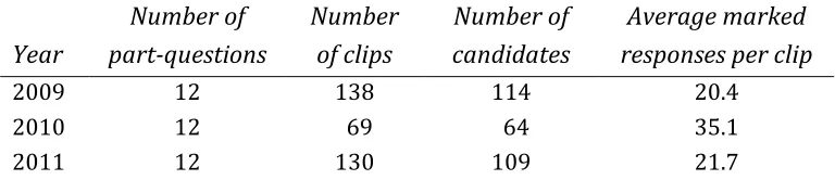
worked (see Table 3). In general, different candidates provided the clips for the different part-questions in the set of seed clips for geography.
Table 3 Clip statistics for geography
Year Number of part-questions Number of clips Number of candidates Average marked responses per clip
2009 12 138 114 20.4
2010 12 69 64 35.1
2011 12 130 109 21.7
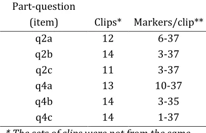
For psychology, the numbers of clips also varied across the years and were also
extremely small (like geography, fewer than 0.2% of all clips in 2011), but this time the number of marked clips was similar across part-questions within a year (since all candidates were required to attempt all the questions in the paper). See Table 4 for details.
Table 4 Clip statistics for psychology
Year Number of part-questions Number of clips Number of candidates Average marked responses per clip
2009 15 313 159 11.5
2010 11 210 89 15.5
2011 14 223 54 20.0
In backreading, team leaders, now acting as marking supervisors, re-mark a proportion of clips (roughly 10% in geography and 6% in psychology in 2011, for example), the clips being selected and delivered to markers at random by the IT clip distribution system throughout the operational marking period. The supervisor either agrees to the original marker’s mark or indicates that it should be replaced. The re-marking is not independent, since the team leader has sight of the original mark. Corrective action can include removing the examiner from the marking process altogether and re-marking the clips already marked by that individual. Whenever clips are re-marked, the mark awarded by the senior marker replaces the original mark.
3.4 The resulting mark distributions
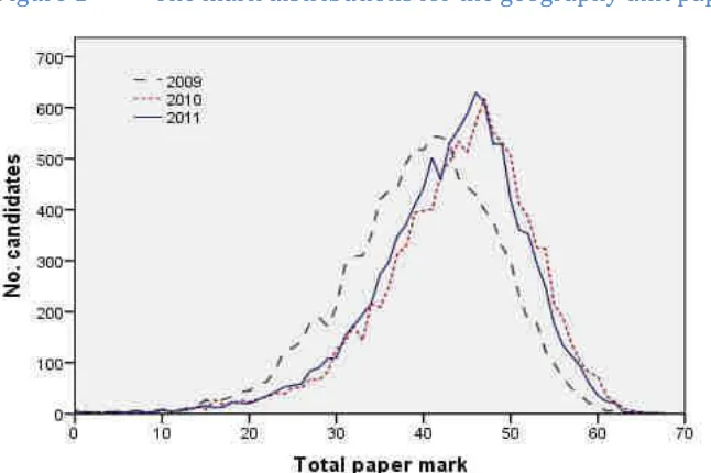
Figure 1 shows the total mark distributions for all three years for geography unit
[image:25.595.67.451.171.254.2]Figure 1 The mark distributions for the geography unit papers 2009-2011
Note in Figure 1 the similarity in the mark distributions for 2010 and 2011 compared with 2009. This is undoubtedly explained by that fact that, as noted earlier in this chapter, the 60-minute time allowance for the paper in 2009 was increased to 75 minutes in 2010. In 2010 and 2011, therefore, candidates had 25% more time in which to respond to the same number and type of extended response questions. This would explain the shift up the mark scale of the 2010 and 2011 mark distributions. The annual standard setting process will have addressed this issue and adjusted grade boundaries accordingly.
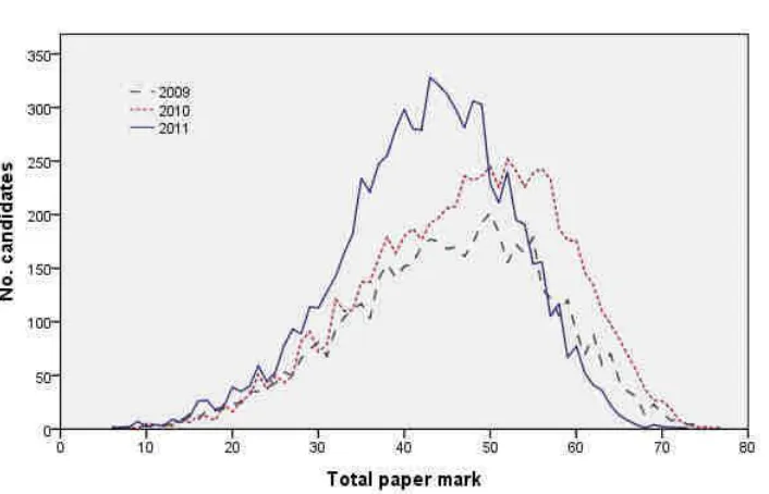
Figure 2 The mark distributions for the psychology unit papers 2009-2011
The critical question for this project is what can we say about assessment quality in this context, in terms in particular of marker reliability?
4
Generalizability theory
4.1 Overview of G-theory
G-theory is of particular interest in the context of this project because it is the only modern theory of measurement that has been developed specifically as a means of investigating and refining our understanding of measurement reliability (and, incidentally, also of validity, the two together being dubbed ‘dependability’). As the originators of G-theory succinctly note: ‘The question of “reliability” ... resolves into a question of accuracy of generalization, or generalizability’ (Cronbach, Gleser, Nanda and Rajaratnam, 1972, p.15, original italics). Specifically, the theory relies on notions of domain and replication to produce estimates of reliability which can be ‘generalised’ to a given defined universe. As Brennan notes,
Generalizability theory enables the investigator to identify and quantify the sources of inconsistencies in observed scores that arise, or could arise, over replications of a measurement procedure. (Brennan, 2001a, p.2)
With particular reference to studies of marker reliability, the use of G-theory has a long and influential tradition. The seminal text of Cronbach et al. (cit), for example, contains an extended analysis of the interactions of raters (there called ‘scorers’) with other conditions of testing in the context of a test of communicative ability in aphasic patients (pp. 161-178), as well as an example of a classroom study involving observers rating both teachers and pupils simultaneously (pp. 194-215). In the literature devoted explicitly to rater reliability, the classic paper of Shrout and Fleiss (1979), cited 7,510 times1, uses the conceptual apparatus of G-theory to disentangle the confusions surrounding six different uses and interpretations of the intra-class correlation coefficient as an index of reliability.
The conceptual basis of G-theory inherits from the classical tradition of reliability theory – with some terminological innovation – the definition of an observed score as the linear combination of true score and measurement error, the partition of observed score variance into true score variance and error variance, and the characterisation of reliability as a function of the proportion of observed variance not due to measurement error. Whereas conventional treatments deal only in two sources of variation in scores, however, observed scores in G-theory are decomposed into linear combinations of as many sources of assessment unreliability as are appropriate to the investigation – candidates, questions, raters, training teams, occasions – and, crucially, of their interactions.
Some of these components will be considered as contributing to the true score and some as engendered by measurement, but there are no fixed rules. Part of an
investigator’s skill lies in determining, within the context of their investigation, how these multiple score components should be partitioned into contributors to true score variance and error variance. In principle, ‘random’ factors are factors that are sampled, and effects associated with these contribute to measurement error, whereas ‘fixed’ factors are not sampled and therefore play no part in measurement error. For a full discussion of this issue see, for example, Cardinet, Johnson and Pini (2010).
To illustrate the principle, consider the complete linear decomposition of an observed score Ycmq of candidate c rated by marker m on question q, as shown in Equation 1.
Equation 1
The terms in with a single subscript on the right hand side of Equation 1 are main effects; those with more than one subscript are the interaction terms, representing the joint effect of components indexed by the subscripts as they act together to influence the observed score. The error term represents any effects that are not captured by the other right-hand-side terms; as such it is often called the residual term. Very few assumptions are needed to support practical application of Equation 1. The main ones are that all of the right-hand-side terms, except , which is always constant, when interpreted as random variables have expected value 0, so that ( ) , and are uncorrelated. No distributional assumptions are made at this stage beyond the requirement that the means and variances exist; in particular there are no normality distributional assumptions.
There are two circumstances under which distributional assumptions might be needed: 1. Many estimation techniques depend on defining a likelihood or prior distribution for
the observations. Whenever possible, ANOVA-based estimation techniques, which only use least squares, are to be preferred. For unbalanced data, as long as the lack of balance is not outrageous, the so-called Henderson methods, otherwise known as analogous ANOVA, give satisfactory results without requiring parametric
assumptions about the distribution of the observed data.
2. Although G-theory is not conceived within an inferential framework (it does not require F-tests to establish model fit, for example), it may be useful to construct confidence intervals around sample mean scores, most commonly based on a
reasonably appeal to the Central Limit Theorem to justify defining the confidence interval (see, for example, Snedecor and Cochran, 1989).
4.2 Variance decomposition
On the basis of these few assumptions, we can define a decomposition of the observed score variance in terms of variance components corresponding to each of the effects in Equation 1:
Equation 2
The development of G-theory – as well as many of the principles of its application in practice – has been from the start heavily influenced by the theory of experimental design, which also has variance analysis as a central theme. Probably as a result of this close association, equations like Equation 1 are more likely to be referred to as designs than models, though it is also the case that hard-core G-theory advocates prefer to eschew the term ‘model’, perhaps to emphasise the paucity of assumptions needed to support a G-theory analysis.
In practice, when we actually apply a design to real observations, it will almost always be the case that we only have available a single observation with which to estimate both
, the interaction of one candidate with one question and one marker, and its variance, , which is clearly not sufficient. In fact, it will in general be impossible to disentangle the highest-order interaction effect from the residual error – the two effects are confounded. Consequently, we will usually write variance component equations like Equation 2 with a single term, which we notate , conflating the last two terms. The new look version of equation Equation 2 would be:
Equation 3
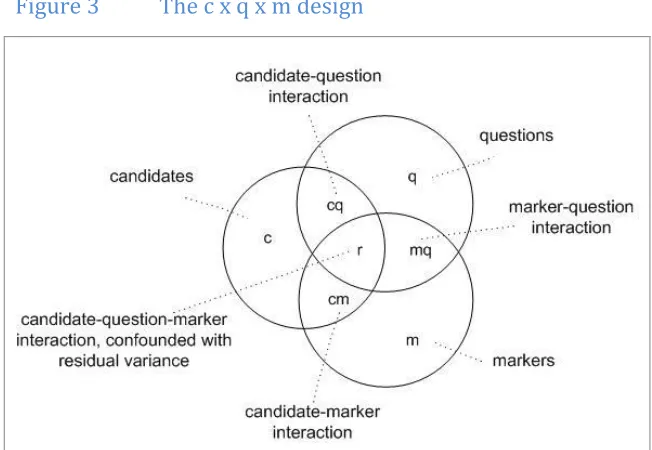
Designs like Equation 1, and the resulting variance decomposition Equation 2, are quite simple by G-theory standards. The proliferation of subscripts and the strings of almost identical symbols can become impossible to read, and the information therein
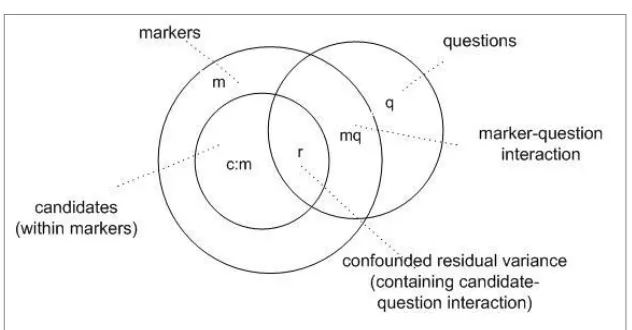
impossible to digest. An alternative representation, the variance component diagram, of which Figure 3 is an example, can be a very helpful visual aid in clarifying the
Figure 3 The c x q x m design
The variance of a main effect is represented as a circle (occasionally as an ellipse when the topology becomes too complex). The intersection of two or more circles denotes the presence of an interaction between both or all of the intersecting effects. Two caveats: these are not Venn diagrams, and the size of a circle is not intended to bear any relation to the importance or magnitude of the component it represents. We make frequent use of these diagrams in the following exposition.
Depending on the aim of the analysis, certain variance sources are considered to be contributing to ’true’ or valid variance and others to error variance, with some making no contribution to either. Classical reliability coefficients are most often constructed as intra-class correlations, ratios of true score variance to the combination of true score and error variance. Generalizability coefficients are a generalisation of the same idea, where designs like Equation 2 are the basis for deciding which linear combinations of variance components represent the valid variance and which the error variance. For further information on the conduct of a G-theory analysis see recent Ofqual reports by Johnson and Johnson (2012a, 2012b).
One of the innovations of G-theory is the recognition of a distinction between relative and absolute error variance. The measurement error variance for the case of ‘relative’ candidate measurement (typically norm-referenced applications) is a linear
Thus the error variances for candidate measurement are: Equation 4
( ) ⁄ ⁄ ⁄
Equation 5
( ) ⁄ ⁄ ⁄ ⁄ ⁄
⁄
where the denominators represent the sample sizes for the different effects.
Similarly, the measurement error variance for the case of ‘relative’ marker measurement (inter-rater reliability) is a linear combination of the interaction
variances involving markers – in Figure 3 these are the candidate-marker interaction variance, the marker-question interaction variance, and the confounded residual variance (hence Equation 6). Again, the measurement error variance for ‘absolute’ marker measurement is a linear combination of these interaction variances and the between-candidate and between-question variances (Equation 7).
Equation 6
( ) ⁄ ⁄ ⁄
Equation 7
( ) ⁄ ⁄ ⁄ ⁄ ⁄ ⁄
From the estimated measurement error variance comes the standard error of measurement (SEM), and from the SEM the 95% confidence interval around a mean score or total score can be produced. What-if analyses can follow, in which the effect on the measurement error variance, SEM and confidence interval of changes in the
measurement conditions can be predicted, by substituting previous factor sample sizes with alternatives. Thus, for candidate measurement we could explore the influence on total score precision of single-marking versus double-marking combined with changes in the numbers of questions in the component paper.
different questions or candidate scripts per marker be changed. We are thus able, provided data collection – the experimental design – has been organised to support extraction of the information we need, to apply the principles of G-theory to quantify the contribution of different sources of score variation to measurement error, and to use the results to identify the optimum future operational strategy for delivering and marking tests (see Wood, 1991; Johnson and Johnson, 2012a, 2012b; Bramley and Dhawan, 2012).
Thus far we have only considered the case of fully crossed designs, where all main effects and all interactions between the main effects are present. In the operational process, however, fully crossed designs typically do not hold. In particular, single-marking of scripts is the norm. This means that the mark data resulting from
operational marking are not useful for estimating the reliability with which candidates will have been measured. The reason for this is that candidates are now nested within markers, so that we no longer have any way of quantifying the impact on candidate measurement reliability of any between-marker variation (which contributes to absolute measurement error) or of any candidate-marker interaction variance (which contributes to both absolute and relative measurement error).
With the notation c:m representing candidates nested within markers, Figure 4 gives the variance component diagram for the c:m x q design. All that can be done in this situation is to ignore the presence of markers in the assessment process altogether, so that ‘markers’ becomes a ‘hidden factor’ in the analysis, and simply look at the impact on candidate measurement error of test questions (using the c x q design, as in many of the application examples offered in Johnson and Johnson, 2012a). Ignoring markers, however, would reduce the validity of the reliability estimation, and cloud
[image:33.595.65.381.568.733.2]On the other hand, the single-marking of scripts does not necessarily of itself have the same devastating effect on marker reliability estimation, if it can be assumed that the candidates nested within markers are interchangeable samples (i.e. similarly
representative of the whole component entry). Random allocation of scripts to markers should achieve this requirement, whereas the allocation of centres to markers, a
common strategy in the days of paper-based scripts, would most likely not do so. If equivalent candidate samples could be assumed then the measurement error variance for relative marker measurement would be a linear combination of marker-question interaction variance, between-candidate (within marker) variance, and confounded residual variance. The between-question variance would be added to the linear combination for absolute marker measurement.
4.3 From script marking to clip marking
But the current situation is that scripts are no longer sent in their entirety to markers, but are decomposed into individual questions or part-questions before being delivered electronically to markers as ‘clips’ for online marking. For marker measurement the situation, while more complicated, is still accessible. Indeed, since randomised allocation of questions or part-questions is the norm, the previous potentially
problematic effect of confounded marker-centre interaction is eliminated. Reliability analysis has simply become more challenging.
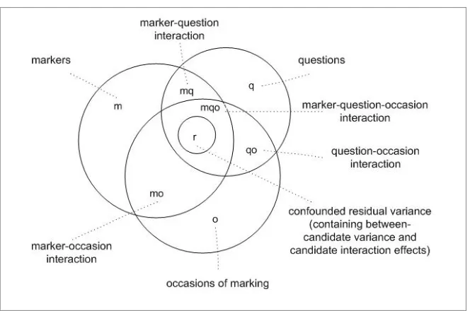
Despite analysis complexity, it would be possible to extend the model to explore the issue of potential marker drift over time. The new analysis design is shown in Figure 5. We have simply added ‘occasions’ to the picture. This extended design allows
Figure 5 The c:(moq) design
But can we say anything about the reliability with which candidates were assessed on an examination component? The answer is only if we have data from a situation where individual candidates were independently marked by more than one marker, as
Bramley and Dhawan (2012) observe:
From a measurement perspective, the ideal scenario for quantifying marker agreement is when two or more markers mark the same piece of work without knowledge of what marks the other markers have given to it (referred to as ‘blind’ double or multiple marking). The marks can then be treated as independent in the statistical sense which is usually an assumption of most common methods of analysing agreement. (Bramley and Dhawan, 2012, p.268) Single-marked clip data from the operational process is not useful for this purpose. Backread data are not useful either, because although each clip is marked by two markers one of these markers, the team leader, has knowledge of the mark awarded by the marker whose marking performance is being checked. The two marks are not, therefore, independently awarded.
Seeded clip data, on the other hand, do have potential for this kind of analysis, given that seeded clips are independently marked by several, and sometimes all, of the
regular markers. Seeded clips are distributed to the regular markers at various points in the operational marking process. The examiners mark these, as they do the other clips that are randomly allocated to them, unaware that they are seeded and therefore pre-marked by a principal examiner.
whole. However, for reasons that will be explained as the results of seeded clip analyses are presented later in this chapter, the data that resulted from the seeded clip
benchmark checks for each of the AS-level papers considered in this project were not ideal for the purpose of estimating component reliability. Analyses are nevertheless reported as illustrations of the potential value of seeded clip data for component
reliability investigation, value that could be maximised by some adjustment to the scope and scale of benchmarking exercises in the future.
All of the reported G-theory analyses featuring markers were carried out using data from experienced regular markers only; the one or two new markers that participated in the marking in one or other year were excluded, as were supervisors, principal and chief examiners. In every case the unit of analysis was the mark given to a single clip by a single marker. Depending on their complexity and the amount of data involved, analyses were carried out using urGENOVA (Brennan, 2001b), mGENOVA (Brennan, 2001c) or SPSS (variance components procedure, for crossed designs with small datasets).
4.4 Geography G-study analyses and findings
As noted in Chapter 3, the geography unit paper carried the same structure and mark tariff pattern across the three years – only the specific question content changed, as did the time allowance, which was increased from 60 to 75 minutes from 2010. The paper comprised two sections, each presenting two three-part questions of which candidates were to choose one. Questions carried 35 marks, for a two-question paper total of 70 marks, with part-questions (e.g. q2a, q2b, q2c) carrying 10 or 15 marks.
Table 5 Candidate numbers for the geography unit paper
Year q1+q3 q1+q4 q2+q3 q2+q4 All* 2009 413 2,585 837 5,504 11,102 2010 415 2,590 800 6,028 10,844 2011 393 2,859 668 6,022 10,980 * Includes some resit candidates, and candidates who attempted at least one part-question over and above a valid combination of six
4.4.1 Marker effects study for geography (operational data)
Table 6 presents the results of the analysis of the single-marked operational data for geography for each of the three years, looking across all 12 part-questions (or ‘items’) in each paper. The underpinning design is illustrated schematically in Figure 5, with the addition of markers nested within teams (imagine Figure 5 with an additional ‘team’ circle encompassing the marker circle). The primary intention was to investigate the possibility that there might be training team and marker drift effects at play, and if so to quantify them. A secondary objective was to estimate the reliability of marker means when calculated over different numbers of clips.
Sequential periods of marking were identified for individual markers so that the possibility of marker drift might be investigated. In general, during the one-month operational marking period, markers were allocated and marked several hundred clips (between 1,280 and 2,740 per marker in 2011) from across all the part-questions in the paper for the year in question. Different markers marked their allocated clips at
different rates (which explains the wide range of clip numbers marked per marker) and over different sub-periods: for example one marker might have marked at a steady pace throughout the month while another might have marked almost all allocated clips within the first two weeks. It would make little sense, therefore, to look at the issue of possible marker drift by dividing the marking month into the same sub-periods for all markers, since some markers would be represented by very few clips for one or other of the four quarter-periods. In the interests of valid interpretation, therefore, four
consecutive marking periods were identified for each marker individually. These were determined by dividing each marker’s clip allocation into quarters over time (clip marking is routinely time-stamped), and rounding the resulting marking periods to one day.
possibly different in real time from one marker to another, has the same meaning for all markers as the earliest marking period, and so on. For this reason we can say that markers are crossed with periods, as they are also crossed with questions (clips are nested within markers, but markers participate in the marking of all the questions in the paper). It is arguable whether ‘periods of marking’ should be considered in analysis as a fixed or a random factor. For ease of analysis we have treated it as random; in the event, given the low variance components associated with the factor ‘periods’ the same results would have arisen had we treated the factor as fixed.
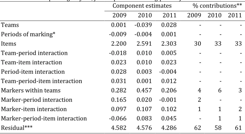
Table 6 Variance breakdown for the single-marked operational datasets for geography
(> 60,000 single-marked clips per year, covering 12 part-questions (items); four teams of 5-8 markers each depending on year, four sequential marking periods)
Component estimates % contributions** 2009 2010 2011 2009 2010 2011
Teams 0.001 -0.039 0.028 - - -
Periods of marking* -0.009 -0.004 0.001 - - -
Items 2.200 2.591 2.303 30 33 33
Team-period interaction -0.018 0.010 0.005 - - -
Team-item interaction 0.023 0.010 0.023 - - -
Period-item interaction 0.028 0.003 -0.004 - - - Team-period-item interaction 0.031 0.001 0.012 - - -
Markers within teams 0.282 0.457 0.206 4 6 3
Marker-period interaction 0.165 0.020 -0.001 2 - - Marker-item interaction 0.097 0.107 0.102 1 1 2 Marker-period-item interaction -0.066 0.083 0.045 - 1 1
Residual*** 4.582 4.576 4.286 62 58 61
* Each marker’s operational marking period (identified by virtue of clip time-stamping) was roughly divided into four sequential ‘periods of marking’ in terms of clip counts ** Rounded percentage contributions of each component to the sum of estimated variance components; only contributions of at least one per cent are shown
*** The residual variance will contain all candidate-related variance contributions, including interaction contributions, confounded with random error
[image:38.595.71.494.296.527.2]
The second and related feature to note is that Table 6 provides no evidence of any marking period effect in the operational data, and neither is there any noticeable evidence of any team effect; this absence of evidence of team and period effects extended to every part-question in the geography papers. It should be noted that had there been strong evidence of a team effect, this would not necessarily have been interpretable as evidence of an influence of team leader training on team members, since it could just as readily have indicated pre-existing dispositions to relative
severity/leniency on the part of the small number, 5-8, of markers who comprised each team in one year or the other.
In each year close to one-third of the total clip score variance is attributable to between-item variance, a phenomenon at least partly explained by the fact that some
part-questions carried mark tariffs of 10 and others mark tariffs of 15. Between-marker differences make a very small contribution to total clip score variance in comparison, at between 3% and 6%. It should be noted that this is what is observed in the dataset. It can only be considered a reflection of genuine differences in markers’ overall standards of judgement (severity/leniency) if it can be assumed that the sets of clips that different markers marked were randomly parallel, and therefore interchangeable. While the automated clip delivery system offered clips to markers in a random allocation process, and each marker did mark a relatively large number of clips, it must nevertheless be recognised that marker standards and clip batch difficulty are confounded in these data.
Around 60% of the clip score variance is residual variance, within which will be several confounded effects associated with the candidates, principal among them the between-candidate variance, the marker-between-candidate interaction variance and the between- candidate-question interaction variance, none of which can be isolated in the single-marked clip-level data.
Table 7 Predicted precision of markers’ mean clip scores in geography
2009 2010 2011 SEM associated with
clip mean score*
across 5 clips 1.09 1.06 1.00 across 15 clips 0.76 0.72 0.66 across 25 clips 0.67 0.63 0.56 * The relative measurement error variance was produced by dividing the residual variance by the relevant clip sample size, and adding to the result the marker-interaction variance components.
In each year, for samples of just five candidates, 95% confidence intervals around
markers’ mean clip scores would be roughly ± 2 marks, reducing to around ± 1½ marks for samples of 15 clips, and reducing again to under ± 1½ marks for samples of 25 candidates. The figures would naturally vary somewhat across different part-questions.
Unfortunately, it is impossible using the operational data analysis results in Table 6 to provide estimates of the reliability with which candidates were measured by the component paper each year, since any variance contributions from candidates, and from candidate interactions with markers, questions, and so on, are confounded in the residual variance (as noted earlier, the single marking of clips renders it impossible to access this information). The best that we can offer in the circumstances are reliability estimates based on analyses in which all possible marker contributions to measurement error are ignored; in the analyses ‘markers’ is a ‘hidden factor’. Since teams and periods of marking have proved to be irrelevant in reliability terms, these can be excluded from further consideration.
The fact that candidates had question choices within each paper demands a separate analysis for each of the possible pathways (questions 1+3, 1+4, 2+3, 2+4). The analysis design is complicated by the fact that the part-questions, the items, carried different mark tariffs: for each choice of question pair (each chosen pathway) four part-questions carry 10 marks each while the other two carry 15 marks each. This means that a
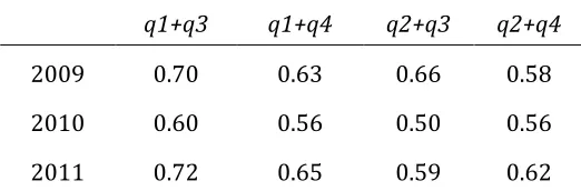
Table 8 Composite score reliability for geography (relative generalizability coefficients)
(design c x (i:t), for candidates by items within tariffs; markers are a ‘hidden factor’, whose effect on reliability cannot here be separately quantified and taken into account)
Pathways through the paper q1+q3 q1+q4 q2+q3 q2+q4
2009 0.70 0.63 0.66 0.58
2010 0.60 0.56 0.50 0.56
2011 0.72 0.65 0.59 0.62
* ‘Tariff section’ weights in analyses were 0.571 and 0.429, respectively, for the 10-mark and 15-mark part-questions.
In line with previous results for similar component papers in other subjects (Johnson and Johnson, 2012a) Table 8 shows modest reliability coefficients for the geography papers, at between 0.5 and 0.7, depending on year and question choice. These are relative generalizability coefficients; coefficients for absolute measurement are very slightly lower in all cases. Alternative analyses that recognised the actual labelled sections in each paper, with three part-questions per geography topic, produced similar results. The question is, how much lower might the coefficients become if we could include marker effects in the analysis? For a possible answer to this question we look now at what the seeded clip data might offer.
4.4.2 Seeded clip analyses for geography
In principle the set of seeded clip data would have been ideal for G-study analysis, following the design illustrated in Figure 3, with ‘questions’ simply replaced by ‘part-questions’. With sufficient data, a single analysis for each year and pathway could have quantified the variance components for markers, part-questions and candidates, as well as for all interactions among these. This information could then have been used in the usual way to meaningfully quantify marker effects, as well as to estimate component reliability for the operational case of single-marking through a what-if analysis.
[image:41.595.67.328.149.235.2]