Flow instability in shock tube due to shock wave-boundary layer-contact surface interactions, a numerical study

ISSN 1450-216X Vol.30 No.1 (2009), pp.164-176 © EuroJournals Publishing, Inc. 2009

http://www.eurojournals.com/ejsr.htm

Flow Instability in Shock Tube Due to Shock Wave-Boundary

Layer-Contact Surface Interactions, a Numerical Study

Al-Falahi Amir

University Tenaga Nasional UNITEN, College of Engineering Jalan Kajang- Puchong, 43009 Kajang

Selangor Darul Ehsan, Malaysia E-mail: alfalahi@uniten.edu.my

Yusoff M. Z

University Tenaga Nasional UNITEN, College of Engineering Jalan Kajang- Puchong, 43009 Kajang

Selangor Darul Ehsan, Malaysia

N. H. Shuaib

University Tenaga Nasional UNITEN, College of Engineering Jalan Kajang- Puchong, 43009 Kajang

Selangor Darul Ehsan, Malaysia

Yusaf T

University of Southern Queensland USQ Faculty of Engineering and Surveying

Toowoomba 4350, Australia

Abstract

This paper describes numerical simulation of transient flow conditions in shock tube. A two dimensional time accurate Navier-Stokes CFD solver for shock tube applications is developed to perform the numerical investigations. The solver was developed based on the dimensions of a newly built short-duration high speed flow test facility at Universiti Tenaga Nasional “UNITEN” in Malaysia. The facility has been designed, built, and commissioned in such a way so that it can be used as a free piston compressor, shock tube, shock tunnel and gun tunnel interchangeably. Different values of diaphragm pressure ratios P4/P1 are applicable in order to get wide range of Mach number.

In this paper, in order to obtain better understanding of the processes involved, CFD simulations were performed for selected cases and the results are analyzed in details. The shock wave motion was traced and in order to investigate the flow stability, details two dimensional effects were investigated. It was observed that the flow becomes unstable due to shock wave-boundary layer-contact surface interactions after shock reflected off the tube end.

1.0. Introduction

It is becoming increasingly difficult to ignore the role of short duration high speed flow test facilities. Recent developments in the field of supersonic and hypersonic applications have led to a renewed interest in this kind of test facilities. Recently, researchers have shown an increased interest in high speed flow conditions which can be used to simulate the real conditions encountered by aerospace vehicles [1]. So far, however, there has been little discussion about the characteristics of the flow process inside these test facilities. Furthermore, far too little attention has been paid to discuss the parameters which affect the velocity profile inside these test facility. Consequently, this has heightened the need for a comprehensive and an integral study which is aided by computer capabilities such as CFD technique. Part of the aim of this paper is to perform a CFD simulation that is able to reveal what is happening for the shock wave generated by high speed flow test facility. The main purpose of this study is to develop deeper understanding of all parameters which affect the shock wave velocity profile and pressure history inside the facility. The short duration hypersonic test facility has been developed recently at the College of Engineering, Universiti Tenaga Nasional (UNITEN). The facility is the first of its kind in Malaysia [2]. It allows various researches to be done in the field of high speed supersonic and hypersonic flows. The maximum Mach number obtainable depends on the type of the driver and driven gases. It is shown that a mach number of 4 can be achieved if CO2 is used as the driven gas and

Helium is used as the driver gas with diaphragm pressure ratio of 75.

2.0. Historical Background

It is informative to trace the history of the shock tube and to note how its use has varied. In the 19th century, interest in the propagation speeds of flame fronts and detonation waves led to the construction of the first shock tube by Vieille in France in 1899 [3]. Experimental work on shock tube has been carried out in the 1940s in the United States and Canada, where initial experiments were made to find a method of blast pressure measurement. It was later realized that shock tubes can be used to investigate compressible flow phenomena and extensive experiments on interactions of shocks, rarefactions and contact surfaces were made in Toronto [3]. Since 1949, the possibilities of using the regions of quasi steady flow to investigate sub and supersonic flow about models, that is, using the shock tube as a very short duration aerodynamic tunnel, have been considered theoretically and practically. It will be noted that the shock tube, which was invented at the same time as the wind tunnel has now developed as a rival to its contemporary. Griffith (1952) [3] at Princeton University has obtained steady flow conditions about a 15º wedge for a range of Mach numbers from 0.86 to 1.16 using conventional wind tunnels. By producing very intense shock waves, relaxation time, ionization and dissociation effects on gas behavior at high temperatures may be studied. Perry and Kantrowwitz (1951) [3], in some preliminary experiments, have observed ionization in argon caused by a converging cylindrical shock, produced by placing “teardrop” in a shock tube of circular cross section. Condensation phenomena in high speed flow have been observed in a shock tube by Wegener and Lundquits (1951) [3], who used air of known humidity in the high pressure compartment and electronically detected the presence of water drops in the flow following the bursting of the diaphragm by the amount of light scatter from the droplets.

3.0. Overview of the Test Facility

Figure 1: Diagram of the test facility

1. Driver section:- A high-pressure section (driver) which will contain the high pressure driver gas, the driver gas can be either Air, Helium, Hydrogen or other light gases.

2. Discharge valve:- To discharge the driver section after each run.

3. Pressure gauge:- To read the pressure inside the driver section, this section is also provided with a static pressure transducer to record the exact value of the driver pressure P4 at which the

diaphragm ruptures.

4. Vacuum pump:- When the driver gas is not Air (e.g. Helium or Hydrogen) then the driver section should be evacuated and refilled with the required driver gas.

5. The primary diaphragm:- This is a thin aluminum membrane to isolate the low-pressure test gas from the high-pressure driver gas until the compression process is initiated.

6. Piston compression section:- A piston is placed in the (driven tube) adjacent to the primary diaphragm so that when the diaphragm ruptures, the piston is propelled through the driven tube, compressing the gas ahead of it. This piston is used in free-piston compressor and gun tunnel tests.

7. Discharge valve:- To discharge the driven section after each run.

8. Vacuum gauge:- To set the pressure inside the driven section to low values (vacuum values) less than atmospheric value.

9. Driven section:- A shock tube section (smooth bore), to be filled with the required test gas (Air, nitrogen or carbon dioxide).

10. Driven section extension:- The last half meter of the driven section on which the pressure transducers and thermocouples are to be mounted.

11. The secondary diaphragm:- A light plastic diaphragm to separate the low pressure test gas inside the driven section from the test section and dump tank which are initially at a vacuum prior to the run.

12. Test section:- This section will expand the high temperature test gas through a nozzle to the correct high enthalpy conditions needed to simulate hypersonic flow. A range of Mach numbers is available by changing the diameter of the throat insert.

13. Vacuum vessel (dump tank):- To be evacuated to about 0.1 mm Hg pressure before running. Prior to a run, the driven section, test section and dump tank are to be evacuated to a low-pressure value.

4.0. Inviscid Transient Flow in Shock Tube

and speed profiles, the code has been validated using two verification approaches. Firstly, the code results have been compared to the Sod’s tube problem (exact solution). Secondly, the code solution is compared with selected experimental measurements for a certain diaphragm pressure ratio. The Sod’s problem [7] is an essentially one-dimensional flow discontinuity problem which provides a good test of a compressible code's ability to capture shocks and contact discontinuities with a small number of zones and to produce the correct density profile in a rarefaction. Further details about the solver can be found in Ref. [8]. CFD solution for inviscid simulation for a diaphragm pressure ratio P4/P1 of 10 has been chosen for a detail investigation. The simulation has been conducted using the actual dimensions of the test facility shown in Figure 1. The pressure, temperature, density and Mach number of the flow were stored in two stations at the end of the driven section with an axial separation of 342 mm as shown in Figure 2.

Figure 2: The two stations at the end of the facility

Station 2 Station 1

wall end Flow direction

Barrel

342 mm 40 mm

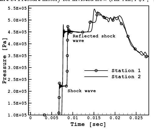
The pressure history for the above mentioned shot is depicted in Figure 3 from which the physics of the flow inside the shock tube can be traced. The first jump represents the shock wave, for which the pressure inside the driven section increases from 100 kPa to around 220 kPa. As the shock wave proceeds to the end of the tube it will reflect and move in the opposite direction increasing the pressure to about 450 kPa. The shock wave will then interact with the contact surface which is following the shock wave and due to this interaction between the shock wave and the contact surface the pressure will be increased until it reaches its peak pressure value of 530 kPa.

Figure 3: Pressure history for inviscid flow (Air-Air, P4/P1=10)

Time [sec]

Pres

sur

e

[Pa

]

0 0.005 0.01 0.015 0.02 0.025

1.0E+05 1.5E+05 2.0E+05 2.5E+05 3.0E+05 3.5E+05 4.0E+05 4.5E+05 5.0E+05 5.5E+05

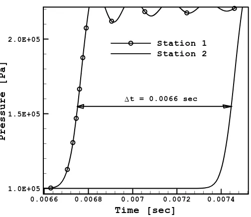
Station 1 Station 2

The shock wave speed can be determined from the CFD data obtained from this simulation. As the distance between the two stations is known (0.342 m) and the time of shock travels from station 1 to station 2 can be obtained from the pressure history graph, as shown in Figure 4, the shock wave speed is determined for this shot is 518 m/s. Comparing to the theoretical value for this pressure ratio (558 m/s) the percentage difference is around 7%. The difference is probably due to the two-dimensional effect which is not modeled by the theoretical solution. From experimental measurements the shock speed for the same pressure ratio is 450 m/s, which indicate percentage difference of about 13% from CFD results. More details about the shock speed measurements can be found in Ref. [9].

Figure 4: Shock wave speed (inviscid flow)

Time [sec]

Press

ure

[Pa]

0.0066 0.0068 0.007 0.0072 0.0074

1.0E+05 1.5E+05 2.0E+05

Station 1 Station 2

t = 0.0066 sec Δ

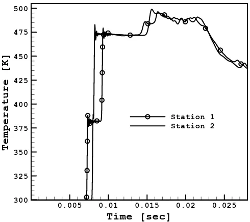
Figure 5: Temperature history inside the shock tube (inviscid flow)

Time [sec]

Temp

era

ture

[K

]

0.005 0.01 0.015 0.02 0.025 300

325 350 375 400 425 450 475 500

Station 1 Station 2

5.0. x-t Diagrams

In order to have overall view of what is happening inside the tube after diaphragm rupture, the x-t diagram for both pressure and density are depicted in Figures 6 and 7 respectively. From these two figures, the inviscid flow process inside the tube is fully described. After diaphragm ruptures a shock wave travels along the driven section followed by a contact surface compressing the test gas inside the driven section causing high pressure and temperature. In the same time a rarefaction waves travel in the opposite direction along the driver section decreasing the driver pressure and temperature. Both shock and expansion waves will be reflected after getting to the end of the tube and the shock wave interacts with the contact surface. It is interesting to note that after interaction with the reflected shock wave, the contact surface remains at about the same position, indicating achievement of the tailored condition. The presence of the bush is also seen to have prevented the rarefaction wave and the shock wave from passing to the other section. The rarefaction wave and the shock wave are reflected when they reach the bush.

Figure 6: x-t diagram for pressure profile (inviscid flow)

0 0.005 0.01 0.015 0.02 0.025 0.03

Ti

m

e

[sec]

0 0.5 1 1.5 2 2.5 3 3.5 4 4.5 5 5.5 6 6.5

Distance [m]

X Y

Figure 7:x-t diagram for density profile (inviscid flow)

0 0.005 0.01 0.015 0.02 0.025 0.03

Time

[sec]

0 0.5 1 1.5 2 2.5 3 3.5 4 4.5 5 5.5 6 6.5

Distance [m] X

Y

Z

6.0. Viscous Transient Flow in Shock Tube

In order to investigate the effect of viscosity on the transient flow in shock tube and how it affects the performance of the facility, a viscous simulation has been accomplished for the same boundary conditions as in inviscid simulation presented in the previous section. The pressure history for the above mentioned shot is depicted in Figure 8. The Figure shows similar trend as for the inviscid flow. The first jump represents the pressure rise due to shock wave, for which the pressure inside the driven section increases from 100 kPa to around 220 kPa. The shock wave then reflects as it hits the end of the tube and moves in the opposite direction subsequently the pressure increases to about 450 kPa.

Figure 8: Pressure history for viscous flow (Air-Air, P4/P1=10)

Time [sec]

Pre

s

s

ure

[Pa]

0 0.005 0.01 0.015 0.02 0.025 0.03 1.0E+05

1.5E+05 2.0E+05 2.5E+05 3.0E+05 3.5E+05 4.0E+05 4.5E+05 5.0E+05 5.5E+05

Station 1 Station 2

shock wave reflected shock wave

The shock wave will then interact with the contact surface which is following the shock wave and due to this interaction between the shock wave and the contact surface the pressure will be increased until it reaches its peak pressure value which is in this case equal to around 530 kPa.

seen that viscosity decreases the shock wave speed to about 11% due to the boundary layer effects. From experimental measurements the shock speed for the same pressure ratio is 450 m/s, which indicate percentage difference of about 1.3% from CFD results.

Figure 9: Shock wave speed (viscous flow)

Time [sec]

P

ressure

[Pa]

0.00675 0.007 0.00725 0.0075 0.00775

1.0E+05 1.5E+05 2.0E+05

Station 1 Station 2 t = 0.00075 sec

Δ

After it hits the tube end, shock wave will be reflected and it will move to the left with a slower velocity which can be determined using the same procedure. The wave speed decreases to about 311 m/s. Comparing with respect to the reflected shock wave speed for inviscid flow which is 342 m/s, it is apparent that viscosity resists the fluid motion causing slower speed of the shock wave by 9.1%.

Analyzing the temperature history for this simulation, it can be seen that the trend is quite similar to pressure history. The temperature results for this run have been displayed in Figure 10. The first jump represents the shock wave and the second jump is due to the reflected shock wave. The temperature is increased from the initial value of 300 K to about 500 K.

Figure 10: Temperature history inside the shock tube (viscous flow)

Time [sec]

Te

m

p

erature

[

K

]

0 0.01 0.02 0.03

300 325 350 375 400 425 450 475 500

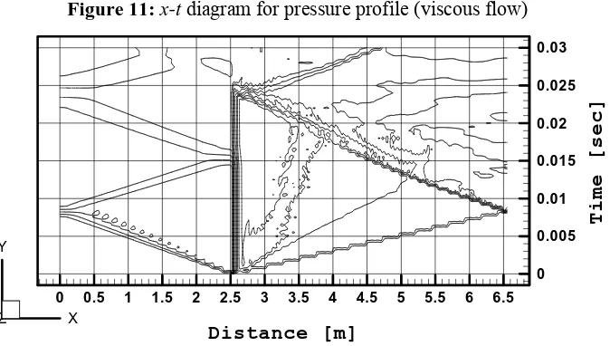
Figure 11 and 12 shows x-t diagram for pressure and density profiles respectively. It can be noted from Figure 12 that the intersection point between the reflected shock wave and the contact surface occurred at 5.35 m as compared to inviscid flow at 5.15 m (as shown in Figure 7); this indicates slower shock speed for the viscous flow and hence confirm the above calculation of shock speed.

Figure 11: x-t diagram for pressure profile (viscous flow)

0 0.005 0.01 0.015 0.02 0.025 0.03

T

i

m

e

[

se

c]

0 0.5 1 1.5 2 2.5 3 3.5 4 4.5 5 5.5 6 6.5

Distance [m]

X Y

Z

Figure 12: x-t diagram for density profile (viscous flow)

0 0.005 0.01 0.015 0.02 0.025 0.03

Time

[sec]

0 0.5 1 1.5 2 2.5 3 3.5 4 4.5 5 5.5 6 6.5

Distance [m]

X Y

Z

Figure 12 shows the so-called tailored interface, where no disturbance is reflected from the contact surface back towards the rear wall of the shock tube. The “tailored” contact surface configuration offers a number of advantages when applied to the operations of shock tubes, it increases the testing-time and it improves the homogeneity of the working gas parameters (i.e. it decreases possible contamination effects in the test section caused by the driver gas).

As shown in Figure 12, the maximum useful duration time that can be obtained when the prescribed pressure ratio P4/P1 =10, is about 10 ms, which is quite comparable to other facilities. The

procedure of calculating the useful duration time (τ) has already been explained in Ref [10].

7.0. Shock Wave - Boundary Layer Interaction

generated near the walls of the shock tube, across which the velocity of the flow decreases from that in the main stream to zero at the walls.

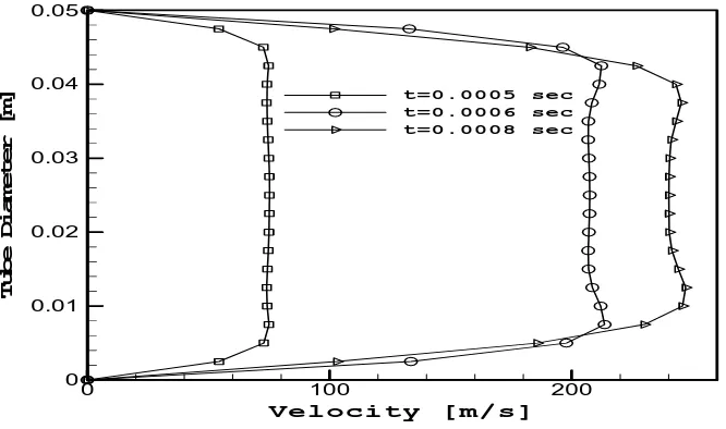
Figure 13 shows the velocity profiles at x = 279 mm from the diaphragm after shock wave passes through it. It can be seen that the boundary layer thickness grows rapidly causing more blockage to the flow. It can be seen from Figure 5.29 that the shock wave speed remains constant as it moves towards the end of the tube. The shock wave speed reduces after reflection but it remains constant until it interacts with the contact surface. After that, there is evidence showing that the shock wave is attenuated and speed reduces. This is due to the effect of the boundary layer on the shock wave which cause additional blockage to the motion. The attenuation of shock wave due to interaction with boundary layer has been reported by McKenzie [11].

Figure 13: Velocity profile after diaphragm rupture (viscous flow) at x = 279 mm from diaphragm section

Velocity [m/s]

Tube

Diameter

[m]

0 100 200

0 0.01 0.02 0.03 0.04 0.05

t=0.0005 sec

t=0.0006 sec

t=0.0008 sec

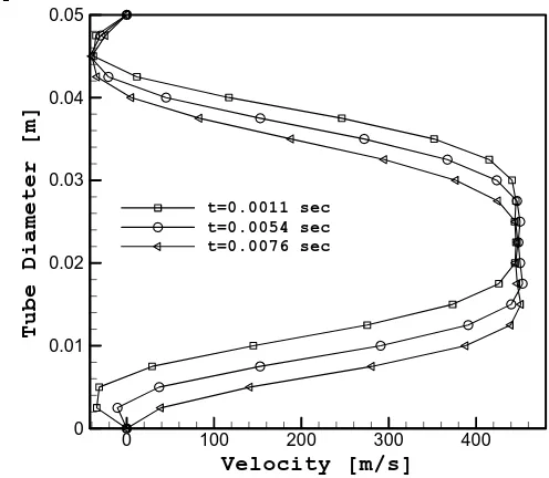
At time t = 0.0011 sec the profile is perfectly symmetrical. However, the velocity profile contains inflexion part, which according to Drazin and Reid [12] is unstable and susceptible to disturbances. The asymmetry becomes more apparent as the process continues. The upper half of the tube has mainly positive velocity whereas the bottom half has negative velocity.

Figure 14: Velocity profile at different times (viscous flow) at x = 279 mm from diaphragm section

Velocity [m/s]

Tu

be

D

iam

et

er

[m

]

0 100 200 300 400

0 0.01 0.02 0.03 0.04 0.05

t=0.0011 sec t=0.0054 sec t=0.0076 sec

Figure 15: Flow after shock reflection at x = 279 mm from diaphragm section

Velocity [m/s]

Tub

e

Dia

met

er

[m

]

-100 0 100 200 300 400

0 0.01 0.02 0.03 0.04 0.05

t=0.0087 sec t=0.0152 sec t=0.0185 sec t=0.0229 sec

Figure 16: Velocity profile after waves interaction at x = 279 mm from diaphragm section

Velocity [m/s]

Tube

Diameter

[

m

]

-100 0 100 200 0

0.01 0.02 0.03 0.04 0.05

After the shock wave reflected and subsequent interaction with the contact surface, the separated flow region evolves into a full re-circulating region rotating in the anticlockwise direction. Then the flow returns back to the small separated flow region close to the tube walls.

The formation of the recirculating region in this simulation is surprising especially considering that the tube is symmetrical. However, it has been reported by Xu Fu et al. [13] that high speed flow tends to become unstable when shock wave interacts with contact discontinuity.

8.0. Conclusion

The paper described the flow process inside a short duration high speed flow test facility built at the college of engineering- Universiti Tenaga Nasional in Malaysia. 2D-CFD solver designed to simulate the flow process inside shock tube. The solver has been applied to a standard case of inviscid flow and it has been validated against standard Sod’s problem and experimental measurements in shock tube. The agreement with the analyzed solution is very good which proved the validity of the basic numerical scheme developed.

References

[1] Al-Falahi Amir ‘Design, Consruction and Performance Evaluation of a Short Duration High Speed Flow Test Facility’ Ph.D. Thesis, Universiti Tenaga Nasional, 2008.

[2] Al-Falahi Amir, Yusoff M. Z & Yusaf T “Development of a Short Duration Hypersonic Test Facility and Universiti Tenaga Nasional”, Journal Institute of Engineers, Malaysia, Vol. 69, No. 1, March 2008, pg. 32-38, ISSN 0126-513X.

[3] B.D. Henshall, “On Some Aspects of the Use of Shock Tubes in Aerodynamic Research”, University of Bristol, Department of Aeronautical Engineering, 1957.

[4] Al-Falahi Amir, Yusoff M. Z & Yusaf T “An Experimental Evaluation of Shock Wave Strength and Peak Pressure in a Conventional Shock Tube and Free-Piston Compressor”, Proceedings of IMECE2008 2008 ASME International Mechanical Engineering Congress and Exposition November 2-6, 2008, Boston, Massachusetts, USA

[5] Zamri, M.Y, “An improved treatment of two-dimensional Two-Phase Flow of Steam by a Runge-Kutta Method”, Ph.D. Thesis, University of Birmingham, 1997.

[6] Zamri M. Y., “A Two-Dimensional Time-Accurate Euler Solver for Turbo machinery Applications” Journal-Institution of Engineers, Malaysia Vol. 5 No. 3 1998.

[7] G. A. Sod, “A survey of several finite difference methods for systems of nonlinear hyperbolic conservation laws”, J. Comput. Phys. 43 (1-31), 1978.

[8] Al-Falahi Amir, Yusoff M. Z & Yusaf T “Numerical Simulation of Inviscid Transient Flows in Shock Tube and its Validations” Proceedings of ICFM 2008: "International Conference on Fluid Mechanics" Heidelberg, Germany September 24-26, 2008

[9] Al-Falahi Amir, Yusoff M. Z, & Yusaf T “An Experimental Technique to Measure the Shock Wave strength and it’s Speed” Proceeding of the International Conference on Construction and Building Technology ICCBT in Kuala Lumpur, MALAYSIA on 16-20 June 2008

[10] Al-Falahi Amir, Yusaf T & Yusoff M. Z “Hypersonic Free Piston Compression Wind Tunnel, Design & Construction”, Proceeding of conference of Advances in Malaysian Energy Research 2004. © 2004Malaysian Institute of Energy and Malaysia Energy Centre. Bangi, Selangor-Malaysia

[11] McKenzie, Nick R., ”The effect of viscous attenuation on shock tube performance”, M.S. Thesis Air Force Inst. Of Tech., Wright-Patterson AFB, OH., 1994.

[12] Drazin, P.G. and Reid, W.H. “Hydrodynamic Stability”, Cambridge Monographs on Mechanics and Applied Mathematics, Cambridge University Press 1993.