RIT Scholar Works
Theses
8-14-2018
Binary Black Holes in the Inspiral Regime: The
Effect of Spins and Eccentricity on Spacetime
Dynamics and Gravitational Radiation
Brennan M. Ireland
[email protected]Follow this and additional works at:
https://scholarworks.rit.edu/theses
This Dissertation is brought to you for free and open access by RIT Scholar Works. It has been accepted for inclusion in Theses by an authorized administrator of RIT Scholar Works. For more information, please [email protected].
Recommended Citation
Ph.D. Dissertation
Binary Black Holes in the Inspiral Regime:
The Effect of Spins and Eccentricity on
Spacetime Dynamics and Gravitational
Radiation
Author:
Brennan M. Ireland
Advisor:
Manuela Campanelli
A dissertation submitted in partial fulfillment of the requirements
for the degree of Astrophysical Sciences and Technology
in the
School of Physics and Astronomy
Ph.D. Dissertation
Binary Black Holes in the Inspiral Regime:
The Effect of Spins and Eccentricity on
Spacetime Dynamics and Gravitational
Radiation
Author:
Brennan M. Ireland
Advisor:
Manuela Campanelli
A dissertation submitted in partial fulfillment of the requirements
for the degree of Astrophysical Sciences and Technology
in the
School of Physics and Astronomy
Approved by
Prof. Andrew Robinson Date
Astrophysical Sciences and Technologies
R
·
I
·
T
College of ScienceRochester, NY, USA
The Ph.D. Dissertation of Brennan M. Ireland has been approved
by the undersigned members of the dissertation committee as satisfactory for the degree of
Doctor of Philosophy in Astrophysical Sciences and Technology.
Dr. Nathaniel Barlow, Committee Chair Date
Dr. Manuela Campanelli, Dissertation Advisor Date
Dr. Richard O’Shaughnessy Date
Observations of black hole binaries via the emission of gravitational waves are one of the most exciting discoveries in physics in the past 50 years. The most generic black holes in nature are ones with spin, which may be misaligned with the orbital angular momentum of the binary, and also orbital eccentricity. This demands computationally inexpensive and accurate models of spinning binary black holes for hundreds of orbits as the binary inspirals.
This dissertation is divided into two projects, both of which focus on binary black holes with spin. In the first project, I construct and present a new global, fully analytic, approximate spacetime which accurately describes the dynamics of nonprecessing, spinning black hole binaries during the inspiral phase of the relativistic merger process. This approximate solution of the vacuum Einstein’s equations can be obtained by asymptotically matching perturbed Kerr solutions near the two black holes to a post-Newtonian metric valid far from the two black holes. This metric is then matched to a post-Minkowskian metric even farther out in the wave zone. The procedure of asymptotic matching is generalized to be valid to all times, instead of a small group of initial hypersurfaces discussed in previous works. I then re-examine the asymptotic matching in the case of precession of the spins, allowing for generically spinning black hole binary metrics. This metric is well suited for long term dynamical simulations of spinning black hole binary spacetimes prior to merger, such as studies of circumbinary gas accretion which requires hundreds of binary orbits.
Abstract i
Declaration v
Acknowledgements vi
List of published work vii
List of Tables viii
List of Figures ix
1 Introduction 1
1.1 Motivation . . . 1
1.2 Introduction to General Relativity . . . 3
1.3 Black Holes and Gravitational Waves . . . 6
1.3.1 Black Holes . . . 6
1.3.2 Gravitational Waves . . . 8
1.4 Observations of Black Holes and Black Hole Binaries . . . 9
1.5 Projects Herein . . . 13
1.5.1 Hybrid Metric Construction for spinning black hole binaries in the inspiral regime . . . 13
1.5.2 Evolution equations for generic black hole binaries . . . 14
1.6 Organization . . . 15
2 Analytic Techniques in General Relativity 17 2.1 The Mathematics of General Relativity . . . 17
2.1.1 Manifolds, Vectors, One-forms, and Tensors . . . 17
2.1.3 Geodesics . . . 19
2.1.4 Curvature . . . 20
2.1.5 Einstein’s Equations . . . 23
2.1.6 Conserved Quantities . . . 24
2.2 Mathematical Properties of Black Holes . . . 25
2.2.1 The Schwarzschild Solution . . . 26
2.2.2 The Kerr Solution . . . 28
2.2.3 Coordinate and Gauge Choices . . . 30
2.3 Approximate Solutions to the Einstein Equations . . . 31
2.3.1 Post-Minkowski Theory . . . 31
2.3.2 Post-Newtonian Theory . . . 36
2.3.3 Black Hole Perturbation Theory . . . 40
2.4 Formulation of Gravitational Radiation . . . 43
3 Construction of an Approximate Global Spacetime with Spin Via Asymptotic Matching 46 3.1 Introduction . . . 46
3.2 Construction of Approximate Global Metric . . . 49
3.2.1 Subdividing Spacetime . . . 50
3.2.2 Inner Zone . . . 51
3.2.3 Near Zone . . . 55
3.2.4 Asymptotic Matching . . . 56
3.2.5 Expansion of the Nonspinning Part of the IZ and NZ Metrics . . . 58
3.2.6 Matching Calculation . . . 59
3.2.7 Global Metric . . . 63
3.3 Numerical Analysis . . . 64
3.3.1 Ricci Scalar . . . 65
3.3.2 Relative Kretschmann . . . 66
3.3.3 Accuracy of the Global Metric: the Ricci Scalar . . . 68
3.3.4 Accuracy of the Global Metric: the Hamiltonian Constraint . . . 75
3.3.5 Aligned Spin . . . 76
3.3.6 Accuracy of the Global Metric: the Relative Kretschmann . . . 78
3.3.7 Numerical Methods . . . 84
3.3.8 Orbital Hang-up Effect, and Long Time Evolutions of the BHB . . . 87
3.4 Discussion . . . 88
3.5 Final Remarks for Non-Precessing Matching Calculations . . . 90
3.5.1 Transition functions . . . 90
3.5.2 Ingoing Kerr Coordinates to Cook-Scheel Harmonic Coordinates . . . 92
3.5.3 Details about the Horizon and the Innermost Stable Circular Orbit . . . 96
3.5.4 Computationally Effective IZ Metric . . . 98
3.6 Asymptotic Matching in the Precessing Case . . . 99
3.6.1 Coordinate rotation . . . 100
3.6.3 Concluding Remarks . . . 104
4 Post-Newtonian Dynamics of Eccentric, Spinning Binaries 105 4.1 Introduction . . . 105
4.2 Formulation of PN Equations of Motion . . . 107
4.2.1 Orbital Position Equations of Motion . . . 107
4.2.2 Spin Precession Equations . . . 111
4.2.3 Quasi-Circular Orbits . . . 113
4.2.4 Eccentricity Definitions . . . 113
4.2.5 The Taylor T4 Method . . . 116
4.3 Gravitational Radiation: T4 and Direct EOM . . . 117
4.4 Comparing to T4 . . . 119
4.4.1 Eccentricity Reduction in the Direct Integration . . . 120
4.4.2 Consistent PN Order in Taylor T4 . . . 122
4.4.3 Quantifying the Comparison: Orbital Frequencies . . . 123
4.4.4 Quantifying the Comparison: Overlaps . . . 130
4.5 Eccentric, Precessing Binaries . . . 135
4.6 Discussion . . . 143
4.7 Final remarks and Tabulated PN Terms . . . 145
4.7.1 T4 Energy and Flux Terms . . . 145
5 Discussion 147 5.1 Summary and Conclusions . . . 147
5.1.1 Validity of the Approximate Analytic Spacetime with Spins . . . 148
5.1.2 Approximate Analytic Spacetime with Precession . . . 148
5.1.3 Comparison of the Direct Equations of Motion . . . 149
5.1.4 Eccentric, Precessing, Binaries . . . 149
5.2 Future Work . . . 150
I, Brennan M. Ireland (“the Author”), declare that no part of this dissertation is substantially the same as any that has been submitted for a degree or diploma at the Rochester Institute of Technology or any other University. I further declare that this work is my own. Those who have contributed scientific or other collaborative insights are fully credited in this dissertation, and all prior work upon which this dissertation builds is cited appropriately throughout the text. This dissertation was successfully defended in Rochester, NY, USA on July 10, 2018.
Portions of this dissertation have been published by the Author in peer-reviewed papers ap-pearing in the Physical Review D (Phys. Rev. D), and Classical and Quantum Gravity:
I first wish to thank my advisor, Manuela Campanelli, for her support, insight, direction, and vision over the past five years throughout my PhD. Her guidance has been invaluable, and her support has been peerless. I would not be who or where I am today without her. To Hiroyuki Nakano, for his mentoring, tutelage, and guidance. To Eric West, for his many collaborative hours spent writing and sifting through code. To Ofek Birnholtz, for his continued encouragement, countless meetings, sanity checks (for both the code and me), and collaboration. To my dissertation committee members, for taking time to serve on my committee and provide guidance and feedback on this work. To my mother Mary, and my father David, for the hours spent reading, writing, teaching, and believing in me as I worked through graduate school. To my sister Keeley for being my best friend. To all of my friends and family who have kept me sane and helped me overcome the tremendous hurdles that accompany graduate school. My sincerest and deepest thanks.
1. Inspiralling, nonprecessing, spinning black hole binary spacetime via asymptotic matching.
Brennan Ireland, Bruno C. Mundim, Hiroyuki Nakano, and Manuela Campanelli (2016, Phys. Rev. D, 93, 104057).
2. Spinning, precessing, black hole binary spacetime via asymptotic matching.
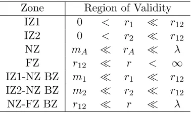
3.1 Regions of validity for the different zones and BZ locations. Here r1 and r2 are the
distances from the first or second BH with massm1orm2,r is the distance from the
center of mass to a field point,r12is the orbital separation, andλis the gravitational
wavelength. For BZs to exist, the system must satisfym1,2r12, though we expect
that the metric will break down before this condition is violated. (This was also presented in Refs. (Gallouinet al.,2012;Mundimet al.,2014;Zlochoweret al.,2015).) 49 3.2 Radius of the marginally stable orbit for various spins in harmonic coordinates. . . . 98
4.1 The overlaps between T4 and EOM methods, documented for different separations, spin vectors, and mass ratios, at both the consistent T4 flux order and the highest T4 fluxes available. There are several interesting lines to pay attention to: as the spins increase in alignment, there is an inflection point aroundχ1 =χ2 = 0.9, where
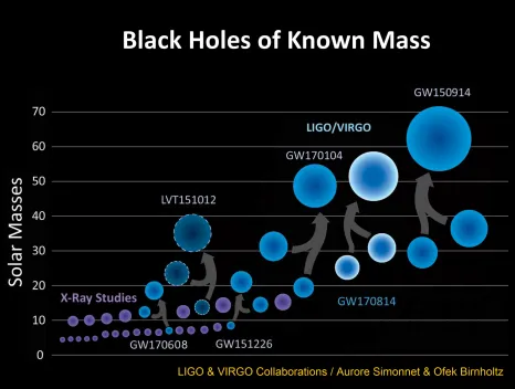
1.1 The black holes of known mass, arranged by ascending mass. The size of the circle indicates visually the value of the mass that is displayed on the y-axis. The purple dots are black hole masses inferred from x-ray studies, the dashed blue circle is a trigger in the LIGO detector that did not achieve the threshold for detection, and the solid blue circles are LIGO detections. . . 10 1.2 A schematic diagram of the detector sensitivities as a function of frequency, along
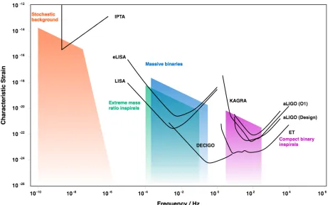
with likely gravitational wave sources in each frequency band. In the low frequency range, pulsar timing (IPTA) sources hope to detect the most massive sources, and the stochastic background of gravitational waves. LISA and eLISA are the next generation space-based detectors, which will target massive binaries, early inspiral LIGO sources, and extreme mass ratio inspirals. DECIGO is another proposed space based detector which will fill the intermediate frequency band, and provide a bridge between LISA and LIGO. aLIGO (O1) is the sensitivity of advanced LIGO for observational run one, and aLIGO (design) is its design sensitivity. KAGRA is the Japanese gravitational wave detector, and the Einstein Telescope (ET) is one of the proposed third generation of gravitational wave detectors. All of these aim for compact binary inspirals such as the detected LIGO sources (Moore et al.,2015). . 12
3.1 A schematic diagram detailing the different zones for the approximate analytic space-time looking down thez-axis at a particular instant in time. The black dots on the
x-axis represent the two BHs, with an orbital separation of r12. The cyan shells
indicate the BZs – regions where two adjacent metrics have overlapping regions of validity. The outermost shell is the NZ-FZ BZ, with both the IZ1-NZ and IZ2-NZ BZs labeled around the individual BHs. The IZ, NZ, and FZ are denoted as the regions contained by the BZs. Note that the circular nature of the BZs is not physical, only schematic, and in general it is expected that they will have some distortions. (This was also presented in Refs. (Gallouin et al., 2012; Mundim et al., 2014; Zlochower
3.2 Comparison of the volume element, √−g, for the global metric for differing values of the spin parameter χ, where both black holes have spin aligned with the orbital angular momentum of the binary. In this plot and the following plots, the horizon is denoted by the grey dashed vertical line, discussed in more detail in Fig. 3.5. The ISCO is the orange dashed vertical line (see final remarks in this chapter 3.5.3 for details). The green dash-dotted vertical lines indicate the boundaries of the different zones, and are consistent for all of the subsequent plots. It is good to note here that the zone boundaries do change for differing spins, though not by much, so here we picked the fiducial zone boundary for theχi = 0.9 (highly spinning) and aligned case. 65
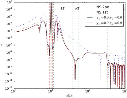
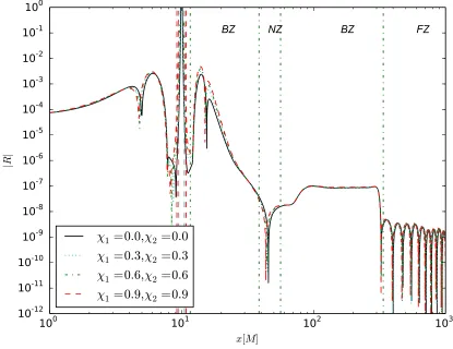
3.3 The absolute value of the Ricci scalar along thexcoordinate, at an initial separation of 20M. We compare here the violations of the Ricci scalar for the spinning BHB metric against the non-spinning (NS) BHB first and second order metrics (Mundim
et al.,2014). It is interesting to note that the new spinning BHB metric has violations of the same order of magnitude as the previous non-spinning BHB metric. . . 69 3.4 The absolute value of the Ricci scalar along x, at an initial separation of 20M. The
spin parameter is varied in this plot. We see that there is little qualitative variation in changing χi. . . 70
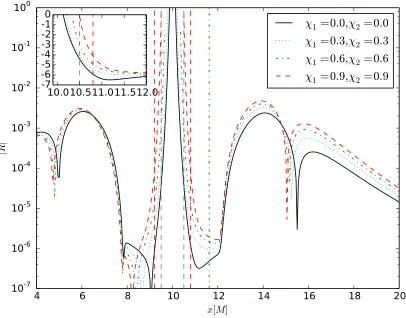
3.5 The absolute value of the Ricci scalar along x, for aligned spins, zoomed in on the inner region near the horizon. The horizon is denoted by the grey dashed vertical line, roughly at a position of xh = xBH,1 ±M/2 on the x-axis, and is easier to
distinguish here than in the previous plots. The ISCO is the orange dashed vertical line (see final remarks 3.5.3 for details). The inset shows the behavior close to the horizon. . . 71 3.6 The absolute value of the Ricci scalar along x, at an initial separation of 20M. This
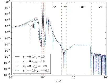
plot shows the spin parameter χi varied for anti-aligned spins. . . 72
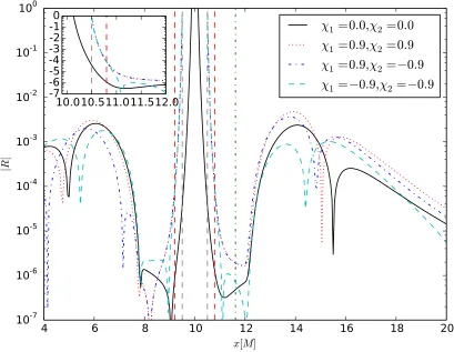
3.7 The absolute value of the Ricci scalar along x, zoomed in near the BH to show the violation near the horizon. This plot shows the spin parameter χi varied for
anti-aligned spins. The inset shows the behavior close to the horizon. . . 73 3.8 The absolute value of the Ricci scalar alongx, at an initial separation of 20M, 12M,
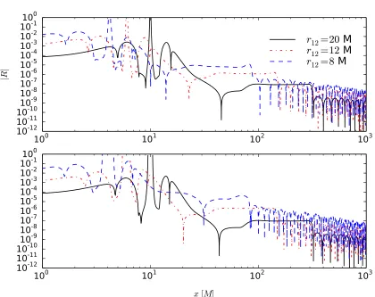
and 8M, for spins χ1 =χ2 = 0.0 (top) and χ1 =χ2 = 0.9 aligned (bottom). Note
that the violation increases smoothly as we decrease in orbital separation. This gives good indication that the dynamics is not introducing any spurious error into the metric. . . 74 3.9 The absolute value of the Hamiltonian constraint along x, at an initial separation
3.10 The absolute value of the Hamiltonian constraint alongx, at an initial separation of 20M, zoomed to focus on the IZ near the BH. Here again the spins are incremented from zero spin to high (χ= 0.9) spin. The inner regions near the BH are similar to the Ricci scalar analysis, including the singularity that is hit just inside the horizon. Again the grey dashed line is the location of the BH horizon, and the orange dashed line is the location of the highly spinning BH ISCO. . . 77 3.11 The Kretschmann invariant calculated for the BHB spacetime for differing values of
spin, all of which are aligned with the orbital angular momentum of the binary, at an initial separation of r12 = 20M. The 1/r6 behavior seen far from the two BHs
(∼40M) is consistent with the value of the Kretschmann in the single Schwarzschild BH case: K = 48M2/r6, where M is the total mass of the binary centered on the origin. The inset shows the behavior close to the horizon, where the spin effects become noticeable. The Kretschmann becomes large as it approaches a BH, because the invariant blows up at a true singularity. . . 79 3.12 The relative Kretschmann for an initial separation ofr12 = 20M, with a grid
reso-lution of 0.0125. In this plot, we are plotting aligned spinning BHs, and increasing the dimensionless spin parameter χi from non spinning to highly spinning. Observe
the normalized behavior that these plots exhibit. The violation to this invariant is very good close to the horizon due to the way that we are normalizing. See Fig. 3.11 for the normalization function. . . 80 3.13 Zoomed in view of Fig. 3.12 around the IZ. The inset shows the behavior close to
the horizon. . . 81 3.14 The relative Kretschmann for an initial separation ofr12 = 20M, with a grid
reso-lution of 0.0125 for varying values of the dimensionless spin parameter χi. In this
plot, we are looking at what the relative Kretschmann does for anti-aligned BHs with high χi values. Observe the normalized behavior that these plots exhibit. The
violation to this invariant is very good close to the horizon, due to the way that we are normalizing. See Fig. 3.11 for the normalization function. . . 82 3.15 Zoomed in view of Fig. 3.14 around the IZ. The inset shows the behavior close to
3.16 Convergence factor along x. Each of the above panels show the Ricci scalar con-vergence factor Q at t = 0 along the coordinate x-axis for different intervals in x, depending on the set of mesh spacing used in the convergence factor computation. On all panels the red dotted line represents the convergence factor for the low resolu-tion mesh spacing set used in that panel, while the blue dashed and black solid lines the medium and high resolution mesh spacing set, respectively. The green horizontal dashed line atQ= 16.0 is the theoretical solution at infinite resolutionh= 0. On the top panel, the low resolution mesh set,hL/M ={0.1,0.05,0.025}, is used to compute QL, while the medium and high resolution ones arehM/M ={0.05,0.025,0.0125}
and hH/M = {0.025,0.0125,0.00625}, respectively. We masked out QH outside
the interval [7M, 13M] to avoid noise due to round-off precision errors. On the sec-ond panel from above, the low resolution set is hL/M = {0.8,0.4,0.2}, while the
medium and high ones are hM/M = {0.4,0.2,0.1} and hH/M = {0.2,0.1,0.05},
respectively. We also mask out QH and QM for x > 25M and x > 35M,
respec-tively, to avoid round-off noise. On the third panel, we use hL/M ={6.4,3.2,1.6}, hM/M = {3.2,1.6,0.8} and hL/M = {1.6,0.8,0.4}. We mask out QH and QM
for x > 90M and x > 140M, respectively. Finally on the bottom panel, we use
hL/M ={51.2,25.6,12.8},hM/M ={25.6,12.8,6.4}andhL/M ={12.8,6.4,3.2}.
These different sets of resolutions were used here to emphasize the mesh spacings required to be in the convergence regime for different zones. . . 86 3.17 The left panel is the orbital hang-up effect shown by plotting the individual
trajec-tories of BH1. Note that the orbits get bunched up as the spin is increased from
χ1 =χ2= 0.0 to 0.9. Both of the BH spins are aligned with the orbital angular
mo-mentum of the binary. The right panel shows the orbital hang-up effect as a decrease in the orbital separation as a function of time for varying aligned spin parameters, with the fiducial spin values chosen to coincide with the spins used in the Ricci and relative Kretschmann analyzes. For both the top and bottom panels, the evolution was terminated at 14000M in time. . . 88
4.1 The difference that an eccentricity definition can make in the calculated eccentricity at a given separation. For this figure, the black holes are non-spinning, start at 20M
separation, and are evolved using the orbital EOMs at low order (equation (2.72a) contains only the 0PN + 2.5PN terms, all others are zero). The eccentricities are then calculated using equation (4.18) (blue) and equation (4.19) (orange). . . 115 4.2 The orbit-adapted vectors for gravitational wave polarizations. N~ is the direction to
the observer, ~p is along the line of nodes, and~q = N~ ×~p. The phase of the binary
φ is defined in a right-handed sense. For the initial conditions, the binary starts on thex axis, and the phase is defined from there. The Newtonian angular momentum
~
4.3 The orbital separation as a function of time over three eccentricity removal iterations. This example is for an initial separation of 20M, with equal masses and no spins. The removal procedure is applied over the first three orbits of the binary, and clearly shows the oscillatory behavior of r(t) decreasing as we apply this removal procedure successively. . . 121 4.4 The time derivative of the orbital separation as a function over eccentricity removal
iterations, for the same configuration as in 4.3. The oscillatory behavior in ˙r is the parameter that we fit and remove in our eccentricity removal procedure. . . 122 4.5 Log of the residuals of ˙r in the eccentricity removal from the data and the model
(4.30), over the first three orbits of evolution to refine the initial conditions. This example is at an initial separation of 20M, with equal masses, and no spins. . . 123 4.6 The relative error of the orbital frequencies as a function of time at different
post-Newtonian orders, starting the binary at an orbital separation of 20M. The orange line is the 3PN term in equation (4.36) minus the Newtonian term, normalized by the 3PN term, so the leading order PN error is 1PN. The green line is 3PN minus 1PN normalized by the 3PN term, so the leading order is 2PN, and the red line is the 3PN minus the 2PN normalized by the 3PN term, so the error is 3PN. The purple line is the relative error of the different orbital frequency definitions for the EOM code, which lays below the 3PN error for the entire evolution. The blue line is the relative error between the 3PN EOM code and the consistent PN order Taylor T4. 125 4.7 The relative difference of the orbital frequencies as a function of time at different
post-Newtonian orders, starting the binary at an orbital separation of 50M. As in 4.6, the orange line is the 3PN term in equation (4.36) minus the Newtonian term, normalized by the 3PN term, the green line is 3PN minus 1PN normalized by the 3PN term, and the red line is the 3PN minus the 2PN normalized by the 3PN term, so the error is 3PN. The purple line is the relative error of the different orbital frequency definitions for the EOM code, which for this separation lies above the 3PN error for the entire evolution. The blue line is the relative error between the 3PN EOM code and the consistent PN order Taylor T4. . . 126 4.8 The relative difference of the orbital frequencies as a function of time at different
post-Newtonian orders, starting the binary at an orbital separation of 100M. As in 4.6 and 4.7, the orange line is the 3PN term in equation (4.36) minus the Newtonian term, normalized by the 3PN term, the green line is 3PN minus 1PN normalized by the 3PN term, and the red line is the 3PN minus the 2PN normalized by the 3PN term, so the error is 3PN. The purple line is the relative error of the different orbital frequency definitions for the EOM code, which for this separation lies above the 3PN error for the entire evolution. The blue line is the relative error between the 3PN EOM code and the consistent PN order Taylor T4. . . 127 4.9 Tracking the PN order of the orbital frequencies as a function of time. We
4.10 A visualization of the data in table 4.1, where we have suppressed all of the spin overlaps, and plot the initial separation vs the log of the mass ratio, with the color scale indicating−log10(1−O). This overlap was done over the shortest evolution, at 20M the simulation ran for only 20 orbits, so the rest of the overlaps were calculated for 20 orbits to give an accurate comparison. This parameterization of the color scale leads to the darker colors indicating a better overlap (the number of nines is indicated on the scale). . . 132 4.11 A visualization of the data in table 4.1, where we have suppressed the mass ratios
and initial separations, and plot the χ1-χ2 plane, with the color scale indicating −log10(1−O). The size of the dot indicates the initial separation, with the larger dots being 50M and the smaller dots being 100M. These overlaps were run on waveforms with a simulation duration of 50 orbits. This parameterization of the color scale leads to the darker colors indicating a better overlap (the number of nines is indicated on the scale). . . 134 4.12 The orbital separation as a function of time for the fiducial system that we lay out
above. The binary has an initial periastron passage of 35M, an initial eccentricity of 0.4, a mass ratio q = 3/2, and initial spin parameter values of χ1 = (−0.3,0,0)
and χ2= (0,0,0.3). The orbital eccentricity as the binary evolves is calculated from
equation (4.21). . . 137 4.13 The individual components of the trajectory as a function of time in the center of
mass variables for the fiducial binary system that we outlined above. The binary has an initial periastron passage of 35M, an initial eccentricity of 0.4, a mass ratio
q = 3/2, and initial spin parameter values of χ1 = (−0.3,0,0) and χ2 = (0,0,0.3).
Note here the spin orbit coupling giving rise to a non zerozcomponent of the orbital motion. . . 138 4.14 The individual components of the total spin vectors as a function of time for the
fiducial binary system that we outlined above. The binary has an initial periastron passage of 35M, an initial eccentricity of 0.4, a mass ratio q = 3/2, and initial spin parameter values of χ1 = (−0.3,0,0) and χ2 = (0,0,0.3). The spin-spin coupling
leads to the spins precessing about the total angular momentum. . . 139 4.15 The plus polarization of the waveform starting with an eccentricity of 0.4, and the
spin vectors χ1 = (−0.3,0,0) and χ2 = (0,0,0.3). The x-axis is time in seconds,
4.16 A zoom plot of the eccentric waveform of the initial few orbits. Thex-axis is time in seconds, where we have dimensionalized the units by using a total binary mass of 25 solar masses. They-axis is dimensionless strainδL/L, where we have calculated the strain with a distance to the source at 500Mpc, and optimal orientation of the binary, as discussed in 4.15. The initial apastron and periastron frequencies are calculated by a peak to peak average of the waveform strain, which is equivalent to an average over 180 degrees of the orbit. The apastron frequency that we calculate is 3.3Hz, and the periastron frequency is 17.3Hz. . . 141 4.17 A zoom plot of the eccentric waveform of the final few orbits. Thex-axis is time in
1
INTRODUCTION
1.1
Motivation
This dissertation focuses on analytic work for understanding and constructing binary black holes
in the most generic case: ones with spins, precessing spins, and eccentricities. The monumental
discovery of gravitational waves from a binary black hole coalescence and colliding neutron stars by
the Laser Interferometer Gravitational Wave Observatory (LIGO) has opened up the field of
grav-itational wave astronomy, providing strong justification for the study of the inspiral and merger of
compact binary systems (both black holes and neutron stars). If we are able to detect non-negligible
eccentricity and spins from a compact binary, this may point us towards a unique formation model
through relativistic 3-body interactions in dense stellar fields, and can tell us specifically about
the last dynamical interaction prior to detection. The modeling of eccentric binaries is relevant to
more than just the LIGO experiment. The third generation of ground based gravitational wave
detectors such as the proposed Einstein Telescope and the Cosmic Explorer will have far better
signal at low frequencies, when the effects of eccentricity will be most pronounced. In addition, the
planned future space based detector Laser Interferometer Space Antenna (LISA) will be sensitive
to accurately predict the outcome of such mergers (D’Orazio and Samsing,2018).
My work is important to the field because we require accurate models that account for all of the
physics present in the merger for the detection of binary black holes. This is an eight dimensional
parameter space, which include generic masses, spins, and orbital eccentricity of the binary. In
the inspiral phase of the binary, many orbits are required to extract physical parameters, which
is impractical for expensive numerical simulations, therefore requiring analytical methods that are
developed in this dissertation. If models for these binaries do not account for physics that is present,
such as eccentricity or spin effects, observational experiments may not be able to find them.
In the case of supermassive black holes that reside in the centers of galaxies (G¨ultekinet al.,
2009), supermassive black hole binaries (BHBs) will form and have additional physics involved.
Specifically, electromagnetic (EM) radiation and gas dynamics become important. I use analytic
techniques to construct a hybrid method for solving the spacetime of these supermassive BHBs to
be used for numerical simulations of gas and EM for many se quential orbits.
Evolving these supermassive black hole systems is a crucial step for our understanding and
study of galactic core dynamics. Galaxies will undergo mergers as the universe evolves (Frenket al.,
1985;Bardeenet al.,1986); therefore, the central supermassive black holes will form a bound pair,
and eventually merge from the emission of gravitational waves. Solving for supermassive black hole
binaries requires evolving the Einstein equations for the black holes, plus the magnetohydrodynamic
equations in a gaseous envrionment (combined, we call this GRMHD) that must be integrated to
dictate how matter moves, what kinds of shocks and accretion can occur, and what electromagnetic
waves leave the system. The spacetime I construct is required for GRMHD simulations to run for
many orbits (potentially hundreds), to study the gas dynamics in sufficient detail to enable EM
observations around supermassive BHBs. The results from these simulations can then be passed
to astrophysicists to look for potential EM signatures from these sources.
The work for my projects requires the extensive use of the theory of general relativity, and
therefore demands a significant amount of discussion to properly motivate. In this chapter, I
such as black holes, black hole binaries, and gravitational waves. I then discuss the projects I
undertook in this dissertation, and layout the overall structure of the dissertation.
1.2
Introduction to General Relativity
Albert Einstein introduced the theory of general relativity to the Prussian Academy of Sciences
on 25 November, 1915, just over 100 years ago. This was based on his realization 1 that “The
outcome of any local, non-gravitational test experiment performed by a freely-falling observer is
independent of the velocity of said observer and independent of when and where the experiment is
conducted”. This is known asEinstein’s equivalence principle.
The laws of physics in general relativity are dictated by the Einstein equivalence principle and
by: 1) the principle of general covariance, a concept that states that the laws governing nature
should be expressible in such a way that they are invariant of the labels that mere mortals (read,
humans) put on quantities to measure them (conventionally called a coordinate system), and 2)
that the laws of physics reduce to those of special relativity when the metric is flat.
Special relativity, described by Einstein in 1905 (Einstein,1905), says that shifts by constant
velocities could be incorporated into a more generic set of transformations - the Lorentz
transfor-mations. Special relativity has two major axioms at its core; the first is that all the laws of physics
are the same in allinertial frames (an inertial reference frame is defined to be an observer that feels
no external forces in its own reference frame. In addition, inertial observers move on geodesics, or
straightest possible paths, of the spacetime2), and the second is the speed of light c must be the
same in all inertial frames.
In general relativity, we adoptgeometric units, where we set the speed of lightc≡299 792 458ms−1
and the universal gravitational constant G≈6.67×10⁻¹¹m3kg−1s−2 equal to 1. These two
rela-tions lead to a conversion between units, such as kg = 6.67×10−11×(3×108)2m, for example.
1
Later he would say that this was his “happiest moment”. 2
When we do this, our units scale out of any given problem. As a nice example of the geometrized
units, take the mass of the sun, 1M = 1.989×1030= 1.477 km = 4.926×10⁻⁶ s, showing us the
conversion from mass to time or distance and vice versa. Physically, we are motivated to use these
units because we wish to mathematically treat space and time equally when formulating general
relativity.
Where indices are used in general relativity, it is implied that we will use the Einstein summation
convention:
ωaVa≡
n
X
a=0
ωaVa=ω0V0+ω1V1+...+ωnVn. (1.1)
Indices in general relativity have four components (three spatial and one temporal), indicating the
coordinates of spacetime. Greek indices (µ= 0...3) represent spacetime indices (with the first index
being the timelike dimension), Latin indices (i= 1...3) represent spatial indices. Generic indices will
be represented by the first letters of the Latin alphabet (a, b, c, ...) where needed. Interchangeably,
we can substitute specific coordinate labels (t, x, y, z), i.e., Vt ≡V0, Gxy ≡G12, and so on. It is
important to note that if indices appear in an expression without being repeated, they are referred
to asfree indices, and if they are repeated (implying that they are summed over), they are referred
to asdummy indices.
Einstein wrote out the field equations for general relativity in tensor equations, which maintain
general covariance 3. From the series of statements that we elucidated above, we can say that the
general relativistic equations that we are seeking couple to matter, and in a local inertial frame
(LIF) it reduces to the spacetime of special relativity, denoted ηµν (this is known as the local
flatness theorem). In a general frame, we adopt the nomenclature metric tensor, and denote it
as gµν, to represent that our spacetime is now curved. Physically, the metric is the “infinitesimal
squared distance” over an infinitesimal displacement. There are many ways in which the metric
is used in general relativity (Carroll, 2004; Sachs and Wu, 1977): it is the tensor that imposes
3He was motivated to use differential geometry by his old classmate Marcel Grossman, and was prompted to
the notions of “past” and “future” (more precisely, we say that it imposes causal structure), as a
squared distance; it allows for computations of path length and the shortest distance between any
two points; it replaces the Newtonian gravitational field Φ =−GM/r, provides us with the notion
of LIFs in general relativity, which allows for the definitions of concepts such as no rotation, and
replaces the Euclidean dot product. In Euclidean coordinates (t, x, y, z), when the spacetime is flat,
the metric tensorgµν =ηµν and is expressible as a matrix as:
ηµν =
−1 0 0 0
0 1 0 0
0 0 1 0
0 0 0 1
.
Here, we are implicitly using another convention for the metric, where thesignature of the metric
(number of positive and negative eigenvalues of the metric) is (−+ ++) 4.
Finally, we must note from the last two statements that while the metric tensor gµν reduces to
the Minkowski metric in a LIF, it must vary from Minkowski globally. We note that this formulation
of general relativity satisfies the Lorentz transformations, and therefore the interval (also referred to
as the line element) in special relativity must holdI ≡ds2 =gµνdxµdxν (in Euclidean coordinates
in flat spacetime, this reduces to ds2=−dt2+dx2+dy2+dz2).
The Einstein field equations couple the spacetime metricgµν (and its derivatives and products
of the metric and derivatives, hidden in the definition of Gµν, which represents the curvature of
spacetime, making the field equations non-linear) to the matter in the Universe via thestress energy
tensor Tµν. To quote physicist John Wheeler, “Spacetime tells matter how to move; matter tells
spacetime how to curve” (Misner et al.,1973). These equations are:
Gµν =
8πG
c4 Tµν. (1.2)
These are a series of coupled, non-linear, second order partial differential equations sourced by the
stress energy tensorTµν. The presence of matter in general relativity therefore greatly complicates
the calculations required to solve anything. A free body in general relativity moves along a
trajec-tory given by its four velocity uµ = dxµ/dλ (built from the familiar three velocity of Newtonian
mechanics with a time component), where λis related to the time experienced by a local observer
moving on this four velocity, and obeys the second order differential equation known as thegeodesic
equation,
d2xµ
dλ2 + Γ
µ νγ
dxν
dλ
dxγ
dλ = 0. (1.3)
The curvature of the spacetime in the geodesic equation is buried inside the Γµνγ symbol. These are
calledChristoffel symbols, or more genericallyconnection coefficients. They are related to curvature
in the coordinates and spacetime. We will explore this more in chapter 2.
1.3
Black Holes and Gravitational Waves
1.3.1 Black Holes
One of the most surprising and fascinating results of general relativity is the concept of a black
hole: that there can exist regions of such strong curvature that not even light can escape. The
concept of a black hole predates general relativity even, with the concept of adark star (Michell,
1784;De Laplace,1808), where the escape velocity of a particle is set to the speed of light, and by
energy balance, we (naively) set potential energy equal to kinetic energy 12mc2 = GmM/R, and
solve forRto obtainR= 2GM/c2, whereM is the mass of the dark star,mis the mass of the test
particle, and R is the distance from the center of the star.
It is, of course, incorrect to assume that energy balance holds (in a Newtonian sense), and that
the escape velocity can be set to the speed of light (forbidden by special relativity). Coincidentally,
this is actually the correct formula for the event horizon of a black hole with no spin and no
surface at which all particles moving at or below the speed of light become trapped 5.
Strikingly, in general relativity, isolated black holes have only three parameters that will
com-pletely characterize their structure. There is a large amount of structure to explore in black holes,
despite being such relatively simple objects. This is known as the “no hair theorem” 6, credited
to John Wheeler for the name, and simply states that the three parameters are the mass M of
the black hole, the electrostatic chargeQ, and the intrinsic angular momentum~a(throughout this
work, we will use the dimensionless spin parameter primarily, defined asχ=|~a|/M2).
To this day, the isolated black hole solutions number only four: the Schwarzschild spacetime
in 1915 (Schwarzschild, 1916), an uncharged, non-spinning black hole; the Reissner-Nordstrom
solution, discovered independently by Reissner (Reissner, 1916), and Nordstr¨om (Nordstr¨om,
1918), which elucidates a charged, non-spinning black hole; the Kerr solution, derived by Kerr
(Kerr,1963), which describes uncharged, spinning black holes; and finally the Kerr-Newman family
of solutions, obtained by Newman et al. (Newmanet al.,1965), which completes the picture with
a description of charged, spinning black holes.
The line element of the most general black hole, the Kerr-Newman solution, expressed in a
coordinate system adapted to the problem, called Boyer-Lindquist coordinates, is:
ds2 = −
∆−a2sin2θ
Σ
dt2−2asin
2θ(r2+a2−∆)
Σ dtdφ (1.4)
+
(r2+a2)2−∆a2sin2θ
Σ
sin2θdφ2+ Σ ∆dr
2+ Σdθ2,
where Σ = r2+a2cos2θ and ∆ = r2 +a2 +Q2−2M r. The parameters of this Kerr-Newman
5This is not quite enough to fully say that we have a black hole. This will be formalized further in chapter 2, when we will discuss that the appropriate definition of a black hole is any region in an asymptotically flat spacetime where it is impossible to escape to future null infinity. For now, we will happily take our naive definition of an object in which nothing, even light, can escape.
6
There are actually no rigorous proofs for the no hair theorem. It has been demonstrated for the Schwarzschild spacetime (Hawking,1971,1972) and the Kerr spacetime (Carter,1971), but a general proof remains elusive (Misner
solution are the mass M, the spin a, and the charge Q, which are exactly the parameters given
by the no-hair theorems. Everything else appearing in the line element above are coordinates and
combinations of coordinates. We can reduce this solution to other black hole solutions (see chapter
2). WhenQ→0, we recover the Kerr solution, whena→0 we reduce to the Reissner-Nordstrom
solution, when Q→ 0 anda→0 we recover the Schwarzschild solution, and whenQ→0, a→0,
and M →0, we obtain Minkowski spacetime in spherical coordinates.
Black holes are formed from total gravitational collapse of bodies, which occurs when an object’s
internal pressure is no longer sufficient to keep it held against gravity. This occurs in stars when
nuclear fusion stops at the end of a star’s life. The loss of pressure support from radiation leads to
gravitational collapse. A spherical solution of the Einstein field equations for a perfect fluid as the
stress energy tensor Tµν yields an upper bound on the mass radius relationship of Mc≤4c2R/9G
before collapse into a black hole becomes an inevitability (Buchdahl,1959).
If the star was not too massive, however, the gravitational collapse can be halted in one of
two states. The less massive stars can have their internal gravitational collapse halted by electron
degeneracy pressure, leading to the formation of a white dwarf, shown by Chandrasekhar originally
to have maximum mass of approximately 1.4 solar masses (Chandrasekhar, 1935; Koester and
Chanmugam, 1990). Once this maximum mass is surpassed, the collapse of the stellar core can
be halted once again by neutron degeneracy pressure, forming a neutron star (Oppenheimer and
Snyder,1939;Oppenheimer and Volkoff,1939;Bombaci,1996;Stergioulas,1998).
1.3.2 Gravitational Waves
The theory of general relativity is rich with fascinating predictions in addition to black holes.
Massive objects that accelerate interact with the spacetime in such a way that they dissipate
energy and momentum in the form of radiation, called gravitational waves. This dissipation is
caused by the rate of change of the mass quadrupole and “mass current” quadrupole and higher
order moments. They propagate in two independent polarizations, travel at the speed of light c,
the distances on one axis and shrinking the distance on the opposite axis, transverse to the direction
of propagation.
There is a plethora of indirect and direct evidence for gravitational waves. The most important
of which is the Hulse-Taylor pulsar (Hulse and Taylor,1975). This binary pulsar system allowed for
very accurate measurements of the decay of the orbit due to gravitational radiation by measuring the
orbital period decay, which agreed with the analytic general relativity prediction to an astonishing
degree. This garnered Hulse and Taylor the Nobel Prize in Physics in 1993.
Several kilometer scale detectors (Abbottet al.,2009,2018) aim to detect these gravitational
waves through laser interferometry, sensitive to one part in 1022 (Martynov et al., 2016; Moore
et al.,2015). The amazing feat of engineering and scientific progress has paid off in full, leading to
the first discovery of gravitational waves from the LIGO scientific collaboration, provided the first
strong evidence of the coalescence of two black holes (Abbott et al.,2016a), which was awarded
the Nobel Prize in 2017, as well as the first coalescence of a binary neutron star system from the
emission of gravitational waves (Abbottet al.,2017a).
The detection of these gravitational wave signals amongst the noisy detector data requires a
strong grasp of gravitational wave theory and knowledge of the radiating sources. Many scientific
resources are being invested to explore the parameter space of possible LIGO sources and to create
efficient model banks for gravitational wave templates (Pan et al.,2014; Taracchini et al., 2014;
Hannam et al.,2014;Santamar´ıa et al.,2010;Khan et al.,2016).
1.4
Observations of Black Holes and Black Hole Binaries
These LIGO measurements constrain the masses and spins of the merging black holes, as well
as the parameters of the remnant merged black hole. To date, there have been five confident
detections of BHBs from the first two LIGO observation runs (Abbottet al.,2016a,b,2017b,c,d),
see figure 1.1. The heaviest component BH had a mass of 36 ± 5 solar masses, with the lightest
which is larger than any X-ray binary that has been detected to date. The individual spins of the
compact binaries are weakly constrained. In particular, only one detection, GW151226, was shown
to have a measurable spin parameter that was not consistent with zero (Abbott et al., 2016b).
The remnants have spins between 0.67 to 0.74, which are not close to the maximal spin allowed. If
the BH spins are misaligned with the orbital angular momentum and the spins precess, additional
features in the waveform can provide even richer studies of the gravitational wave (GW) signature
[image:30.612.74.540.255.607.2](Barker and O’Connell,1987;Kidder,1995).
The likely sources of BHB GW sources are massive low-metallicity stars and globular clusters.
Large low metallicity stars are likely to form compact binaries with the spin axes mostly aligned
with the orbital angular momentum (Belczynskiet al.,2016). BHBs forming in dense clusters will
have no such correlation between the spins and angular momentum, and likely go through strong
perturbing interactions, due to their environment (Rodriguezet al.,2016). These include
super-nova kicks in globular clusters, dense stellar environments, and even 3-body and relativistic-capture
effects. These effects can impart a small but occasionally significant eccentricity, whose
measure-ment provides a unique tracer of the last strong external dynamical effect prior to merger. Future
GW measurements can therefore provide a remarkable opportunity to measure this eccentricity,
and thereby constrain formation scenarios of BHBs.
These constraints will also improve as we move into the third generation of gravitational wave
detectors, where the sensitivity to BHB sources is so high that we expect to be able to capture GW
signals from merging BHBs beyond a redshift of 20 (Vitale and Evans, 2017). This will allow us
to study in detail the parameters of these sources, and we will be able to put much more restrictive
constraints on the BH parameters, as well as potentially finding more unique sources, such as ones
with residual eccentricity.
Future space-based GW missions will target supermassive black hole sources, such as the
pro-posed European Laser Interferometer Space Antenna (eLISA) (Amaro-Seoane et al.,2013a, 2012,
2013b) and the DECi-hertz Interferometer Gravitational wave Observatory (DECIGO) (Setoet al.,
2001), which are sensitive to such low frequency (millihertz band) events, but are a few decades away
from launch. Fortunately, in the case of supermassive black hole binaries, highly-relativistic
mag-netized gas could flow around the pair, as well as around each black hole companion (Bowenet al.,
2017). Therefore, powerful EM signals should accompany the inspiral and merger of BHBs (Roedig
et al.,2014;Schnittman,2013), unlike in stellar-mass BHBs, which are not expected to have any EM
counterparts (Abbott et al., 2016c). This opens a complementary window into the supermassive
sources, in which we can couple GW observations with EM signatures.
grav-Figure 1.2: A schematic diagram of the detector sensitivities as a function of frequency, along with likely gravitational wave sources in each frequency band. In the low frequency range, pulsar timing (IPTA) sources hope to detect the most massive sources, and the stochastic background of gravitational waves. LISA and eLISA are the next generation space-based detectors, which will target massive binaries, early inspiral LIGO sources, and extreme mass ratio inspirals. DECIGO is another proposed space based detector which will fill the intermediate frequency band, and provide a bridge between LISA and LIGO. aLIGO (O1) is the sensitivity of advanced LIGO for observational run one, and aLIGO (design) is its design sensitivity. KAGRA is the Japanese gravitational wave detector, and the Einstein Telescope (ET) is one of the proposed third generation of gravitational wave detectors. All of these aim for compact binary inspirals such as the detected LIGO sources (Mooreet al.,2015).
itational wave astronomy. With LIGO sensitivities getting better as the observing runs continue,
future detectors on the way (both in space and on the ground) (see figure 1.2), and complementary
EM signatures predicted for supermassive sources, it is an exciting time for both gravitational wave
astrophysics and multi-messenger astronomy. These detections provide an excellent opportunity
[image:32.612.74.538.98.386.2]1.5
Projects Herein
The Einstein field equations are an incredibly complex set of non-linear, coupled partial
dif-ferential equations. Unless we have a very high degree of symmetry (which we will define more
rigorously in chapter 2), solving for an exact solution of the field equations analytically is nearly
hopeless. All of the black hole solutions listed above have symmetries that can be exploited. When
we transition to look for BHB solutions, there are no such symmetries, and no exact solution for
the entire spacetime exists, unless we invoke numerical relativity. The advent of numerical
rela-tivity (NR) in 2005 (Pretorius, 2005; Campanelli et al., 2006a; Baker et al., 2006) has allowed
for accurate evolution of the black holes from close separations through merger. When the black
holes are sufficiently far apart, however, numerical relativity is too computationally expensive to
be used. For this, we turn to approximate analytic methods which work well when the bodies are
in this regime (Blanchet, 2014;Will, 2011). This allows us to accurately model the evolution of
the binary as it evolves from early inspiral to eventual plunge and merger, which provides strong
arguments for studying analytic techniques to solve the binary black hole problem.
1.5.1 Hybrid Metric Construction for spinning black hole binaries in the
inspi-ral regime
In the first part of this dissertation, we use several analytic techniques to construct a new, fully
analytic spinning binary black hole spacetime in the inspiral regime for the first time (Ireland
et al.,2016;Nakanoet al.,2016).
The construction of the approximate global metric with spin for a BHB pair on a quasi circular
inspiral, in the inspiral regime, requires us to consider four zones of approximation for a complete
picture: the inner zone (IZ) around black hole 1 (IZ1) and around black hole 2 (IZ2), the near zone
(NZ) around the two BHs, and the far zone (FZ) or wave zone farthest out.
Stitching together these different approximations necessitates using a mathematical process
are valid. The first challenge is deriving the correct matching conditions, then performing the
asymptotic matching to relate the parameters and coordinates of one (say the IZ around BH1) to
the other (say the NZ around both BHs).
We verify the validity of our constructed solution of the Einstein equations in several ways
by looking at invariant quantities such as the Ricci scalar, relative Kretschmann invariant, and
Hamiltonian constraints. All the invariant quantities vanish for an exact solution to the vacuum
field equations (no matter), both at initial times, and as the metric evolves dynamically, observing
known spin effects such as the orbital hang-up effect.
Once precession is taken into account, we need to consider a rotation of each individual IZ
metric from the Kerr metric where the z-direction specifies the spin direction, to a frame where
the z-direction is oriented along the orbital angular momentum and the spins are rotated by Euler
anglesY(Θ) and Z(Φ) to account for the misalignment.
The matching calculations carried out in the precessing case are done to first order in the
matching parameter m2/r12 (more on this later). Second order matching will pick up the time
dependence of the Euler angles Θ and Φ, as well as their derivatives. As such, we expect the higher
order matching will have completely different transformations, which cannot be described by a
simple extension of the nonspinning case, due to the precession of spins.
1.5.2 Evolution equations for generic black hole binaries
In the second part of this dissertation, we develop and calculate the gravitational waveforms and
orbital dynamics from generically spinning, eccentric BHBs. As of now, there are no efficient ways
to calculate waveforms for generic binaries. While it is not expected that LIGO sources in isolated
binaries have significant eccentricity in band, binaries in dense stellar clusters, may however, have
significant eccentricity from dynamical interactions prior to entry into the LIGO band (Rodriguez
et al.,2018).
We use the Lagrangian formulation of the post-Newtonian (PN) equations of motion (EOM) in
Marsat, 2015; Blanchet, 2014; Faye et al., 2006; Blanchet et al., 2006; Marsat et al., 2013; Bohe
et al.,2013).
Up to 3.5PN (A PN order N is said to be a term of order (v/c)2N) order in this PN
formal-ism, and for maximal spin (|χ~a| '1), spin-orbit effects contribute to the EOM at 1.5PN, 2.5PN,
and 3.5PN. Spin-spin effects contribute at 2PN and 3PN. Cubic-in-spin effects start from 3.5PN.
Quartic- and higher order in-spin effects are beyond 3.5PN. Following (Will,2005;Blanchetet al.,
2006;Blanchet,2014), we use the Tulczyjew spin supplementary condition (SSC) to define a spin
vector with conserved Euclidean norm. For this SSC, the higher order spin-orbit terms have been
derived in (Fayeet al.,2006;Blanchetet al.,2006;Marsatet al.,2013;Boheet al.,2013;Blanchet,
2014). The next-to-leading order spin-spin terms were derived in (Bohe et al., 2015), and the
leading order cubic-in-spin terms were derived in (Marsat, 2015). To date, leading order
quartic-and quintic-in-spin contributions to the EOM have not been derived in post-Newtonian harmonic
coordinates with this SSC.
This Lagrangian formulation has larger applications as well. Current preliminary work is being
carried out to see if detection of eccentric sources will be possible, and current prospects look
good (D’Orazio and Samsing, 2018; Breivik et al.,2016;Sesana,2016). By developing a general
EOM that can handle arbitrarily precessing and eccentric BHs, we can apply these EOMs to the
precessing spacetime developed in previous work (Nakanoet al.,2016). We must have an accurate
EOM for the general precessing BHB that can handle the orbital plane precession of the binary
due to spin coupling with the orbit, and also the individual spins precessing in order to evolve the
BHB. The Lagrangian formulation excels at all of these, and can directly be used for this evolution
in the harmonic gauge.
1.6
Organization
The remaining chapters of this dissertation are broken down as follows. In Chapter 2, the
post-Newtonian and post-Minkowskian expansions, black hole perturbation theory, and
gravita-tional wave generation from compact binaries are outlined. Chapter 3 describes the approximate,
analytic metric for black hole binaries with aligned, counter-aligned, and precessing spins. Chapter
4 formalizes and tests the equations of motion for generic black hole binaries in the inspiral regime,
focusing on comparisons with other known methods and numerical relativity. Chapter 5 concludes
2
ANALYTIC TECHNIQUES IN GENERAL RELATIVITY
2.1
The Mathematics of General Relativity
2.1.1 Manifolds, Vectors, One-forms, and Tensors
To mathematically express gravity not as a force, but ascurvature, we are led to use differential
geometry. A manifold is a topological space, a mathematical object that locally “looks like”
Eu-clidean space of dimensionn, represented via real coordinate spaceRn. More precisely, a manifold
is a union of open balls inRn that can be stitched together smoothly.
Manifolds can be embedded with additional structure. A vector is a geometric object, defined
at a pointp, which exists in the tangent spaceTp (which has the same dimensionality asM) as the
directional derivative of curves passing throughp. A vector is represented in a basis through basis
vectors~ea, with components Va. A representation of a vector V~ in a basis is therefore V~ ≡Va~ea.
We can change the coordinate system for a vector using a Jacobian, which, in our summation
convention notation, (see chapter 1) is represented as:
Va0 = ∂x
a0
∂xaV
Recall here that indices used at the beginning of the latin alphabet a, b, c, ... are used as generic
indices, so we have not specialized to four dimensions here yet.
We can equivalently define thedual vectors(which are interchangeably referred to as one-forms),
which live in the dual vector space, or cotangent space Tp∗. A dual vectorω can be represented in
a coordinate system as ω ≡ωaθa, where θa is understood to be the dual basis vectors (analogous
to the basis vectors~ea, but living in the tangent space Tp∗ as opposed toTp).
A tensor is a geometric object that takes copies of vectors and one-forms and returns numbers.
It can be represented in a basis with components, like vectors and one-forms.
The tensor transformation law is a straightforward generalization of the vector and one-form
transformation law, which is (keeping careful track of our indices):
Ta01...a
0 k
b0
1...b0l = ∂xa01
∂xa1...
∂xa0k
∂xak
∂xb1 ∂xb01
...∂x
b l ∂xb0l
Ta1...ak
b1...bl. (2.2)
A key result of the tensor manipulations that we have formalized is that any tensor equation
can be written implicitly in terms of a basis. For instance, if we look again at the Einstein field
equations (1.2),
Gµν = 8πTµν, (2.3)
we understand that this equation is in the ~eµ⊗~eν basis. Looking at an alternate form of the
geodesic equation,
uµ∇µuν = 0 (2.4)
reveals this to be in the~eν basis, and so on. But these bases are arbitrary, so therefore these tensor
equations can be written in any coordinate system with ease. This is a beautiful manifestation
of the principle of general covariance, which we recall was one of the basic founding principles of
2.1.2 The Covariant Derivative
We wish now to represent curvature on a manifold imbued with a metricg(which we will assume here to be Lorentzian, as the theory of general relativity has a Lorentzian manifold structure). The
first step is to define a derivative that is also manifestly covariant.
Thecovariant derivative for a given metric in terms of the ordinary partial derivative is defined
as:
∇µtν =∂µtν + Γνµλtλ, (2.5)
where the Γν
µλ’s are called theChristoffel symbols, and are given by:
Γγαβ = 1 2g
γδ(∂
αgβδ+∂βgαδ−∂δgαβ). (2.6)
These Christoffels modify the ordinary partial derivative to remain manifestly covariant.
A final important note is metric compatibility. The covariant derivative operator is metric
compatible, i.e., it satisfies:
∇γgαβ = 0. (2.7)
2.1.3 Geodesics
The concept of a geodesic is an intuitively simple one: it’s the “straightest” line between two
points. It is the differential geometry extension of the Euclidean intuition that the shortest distance
between any two points is a straight line.
We use the idea of parallel transport of a vectorvα to define a geodesic. This vector is said to
be parallel transported along a curveC with tangent vector tβ if
tβ∇βvα= 0 (2.8)
Given a metric compatible derivative ∇a, we define a geodesic to be a curve whose tangent
vector is parallel propagated along itself, i.e.,
Va∇aVb = 0. (2.9)
Such a geodesic that satisfies equation (2.9) is said to be affinely parameterized with affine parameter
λ1. Writing this equation out in a coordinate basis, and expanding the tangent vector of the curve
asdxµ/dλ, we obtain our result from chapter one, equation (1.3):
d2xµ
dλ2 + Γ
µ νσ
dxν
dλ
dxσ
dλ = 0. (2.10)
Geodesics also have the property of extremizing the path length between any two points. For a
curve C (that is differentiable) on a Lorentzian manifold M with gab, we can define the length of
C as:
l=
Z
(gabVaVb)1/2dλ (2.11)
for spacelike curves (a spacelike vector field obeys gabVaVb >0), and a length of
τ =
Z
(−gabVaVb)1/2dλ (2.12)
for timelike curves (gabVaVb <0 for timelike vector fields). Both of these imply a length of zero
for null (lightlike) curves (gabVaVb = 0 for null vector fields). We have replaced the length l in
timelike curves with a timelike variableτ, which we refer to as theproper time.
2.1.4 Curvature
We can now rigorously define the concept of curvature, using the concept of parallel transport.
The vectorvbwhich we obtain by parallel transporting the vectorva, will, in general, be dependent
on the curve that connects them. When we consider a small closed path to parallel transport a
dual vector, and, upon returning to the starting position, the orientation of the vector has changed,
we say that the surface is curved. If there is no change in the direction the vector is pointing, we
say that the surface is flat. Examples of two dimensional curved surfaces abound. Every ball has
positive curvature, whilst a saddle is negatively curved 2. It is the failure of successive covariant
derivative operations to commute when applied to a one-form that defines curvature.
Curvature can be represented by a tensor called the Riemann curvature tensor. Expressed in a
coordinate basis, the Riemann tensor takes the form:
Rαβµν =∂µΓανβ−∂νΓαµβ+ ΓαµξΓ
ξ νβ−Γ
α νξΓ
ξ
µβ. (2.13)
In a covariant formalism, the Riemann tensor satisfies:
∇a∇bωc− ∇b∇aωc=Rdabcωd. (2.14)
This is the mathematical expression of parallel transporting the one-formωc around a small closed
loop and comparing the action of the metric compatible covariant derivatives ∇a and ∇b stated
above. The consequence of the curvature is best illustrated via geodesic deviation:
Aµ=RµναβPνPαNβ, (2.15)
for initially tangent vectors Pν and deviation vectorsNβ. This shows that the Riemann tensor is
directly responsible for the relative acceleration of geodesics. The relative acceleration of geodesics
Aµ = 0 if, and only if, the Riemann tensor Rµναβ = 0. This is a fundamental result, and shows
clearly observable effects of curvature (which will be shown later).
The Riemann curvature tensor has the following key properties:
• Rdabc=−Rdbac.
• Rd[abc]= 0.
• For the metric compatible covariant derivative ∇c, implying ∇cgab= 0, we have:
Rabcd =−Rabdc.
• The identity:
∇[aRebc]d= 0 (2.16)
holds. This is called theBianchi identity.
As with any tensor, we can decompose the Riemann tensor into the “trace” (contracted) part,
and the “trace free” part. The trace of the Riemann tensor (contracting over the second and fourth
indices) yields theRicci tensor:
Rbabc=Rac. (2.17)
By the symmetry properties of the Riemann tensor above, the Ricci tensor is symmetric:
Rac =Rca. (2.18)
The scalar curvature, orRicci scalar, is defined by the trace of the Ricci tensor:
Raa =R. (2.19)
This is especially useful when looking at errors in spacetimes, because this quantity is coordinate
tensor is called theWeyl tensor, and is defined on 4-dimensional manifolds as:
Cabcd=Rabcd−(ga[cRd]b−gb[cRd]a) +
2
3Rga[cgd]b. (2.20)
The Weyl tensor satisfies the first three properties of the Riemann tensor, as well as being trace
free on all its indices (any contraction of the Weyl tensor is zero).
Another extremely potent tensor is taken by contracting the Bianchi identity equation (2.16):
∇aGab= 0, (2.21)
where the tensor in the derivative is called theEinstein tensor:
Gab≡Rab−
1
2Rgab. (2.22)
The Einstein tensor is symmetricGab =Gba, as its constituent tensors are symmetric, along with
being divergence free from the Bianchi identity.
2.1.5 Einstein’s Equations
The Einstein field equations (already alluded to in (1.2)) are defined as:
Gab≡Rab−
1
2Rgab= 8πTab. (2.23)
Taking the trace of both sides of the Einstein equations yields:
R=−8πT. (2.24)
When we consider a vacuum solution to the Einstein equations, we set Tab = 0, which implies
R= 0, and reduces the field equations to
We will be making extensive use of this fact in our later analysis.
2.1.6 Conserved Quantities
Unfortunately for all physicists (and a relief to everyone else), the real world is a horribly
complicated and messy place. To find a metric that perfectly encapsulates the Universe (or even a
pathetically small piece of it) is nearly impossible. To do so requires a high degree of symmetry to
the problem we are considering, and therefore a way to characterize said symmetry.
Specifically, we seek isometries in our spacetime3. A clear example of these isometries we seek
is:
∂agbc= 0, (2.26)
which expresses that the metric is independent of the xa coordinate. This has a consequence on
geodesics in this spacetime. From the geodesic equation on the four momentum of a timelike
particle
pa∇apb = 0, (2.27)
and expressing in terms of the connection, we obtain:
mdpa
dτ =
1
2(∂agbc)p
bpc, (2.28)
which implies that when we have an isometry, the four-momentum componentpa is a constant of
the motion:
dpa
dτ = 0. (2.29)
This is extremely powerful, as well as useful, and we would like a way of searching for these
isometries. Consider a vector ∂a, which for the moment we will label as K. We say that K
generates the isometry, which physically means that the transformation we can make where the
geometry is invariant can be expressed as an infinitesimal motion in the direction ofK, i.e.,
pb =Kapa=Kapa. (2.30)
But as we’ve already found, the constancy of this quantity is the statement that the directional
derivative along the geodesic vanishes. The only vector Ka that could keep the quantity Kapa
conserved along a trajectory obeysKilling’s equation (Carroll,2004):
∇(aKb) = 0↔ ∇aKb+∇bKa= 0. (2.31)
The vector fields Ka are called Killing vector fields, or simply Killing vectors. Each Killing vector
in a spacetime implies a conserved quantity in that spacetime. We can understand this physically
by again appealing to the constancy of the metric under one of these Killing vectors. This means
that a free falling particle will not feel any forces in the direction of the Killing vector, and therefore
the component of its momentum will be conserved in that direction. These Killing vectors are of
utmost importance in finding and defining conserved quantities in black holes, which we will now
study.
2.2
Mathematical Properties of Black Holes
Black holes are solutions to the Einstein equations, where light cannot escape to infinity. More
precisely, in an asymptotically flat spacetime (a spacetime where the curvature vanishes as we
approach infinity, so the metric approaches the Minkowski metric), if it is impossible to escape to
future null infinity 4, then we characterize that as a black hole 5. This implies the presence of a
physical singularity in the spacetime.
4
denoted asI+
An important characteristic of black holes is that they obey the cosmic censorship conjecture,
which states that the complete gravitational collapse of any body will always result in a black hole,
and not a naked singularity. This means tha