Rochester Institute of Technology
RIT Scholar Works
Theses Thesis/Dissertation Collections
12-19-2017
An alternative episode of care characterization for
supporting the implementation of cluster-based
bundled payment
Amit Singh [email protected]
Follow this and additional works at:https://scholarworks.rit.edu/theses
This Thesis is brought to you for free and open access by the Thesis/Dissertation Collections at RIT Scholar Works. It has been accepted for inclusion in Theses by an authorized administrator of RIT Scholar Works. For more information, please [email protected].
Recommended Citation
Rochester Institute of Technology
An alternative episode of care characterization for supporting the
implementation of cluster-based bundled payment
Thesis
Submitted in partial fulfillment
of the requirements for the degree of
Master of Science in Industrial and Systems Engineering
In the
Department of Industrial & Systems Engineering
Kate Gleason College of Engineering
By
Amit Singh
DEPARTMENT OF INDUSTRIAL AND SYSTEMS ENGINEERING
KATE GLEASON COLLEGE OF ENGINEERING
ROCHESTER INSTITUTE OF TECHNOLOGY
ROCHESTER, NEW YORK
CERTIFICATE OF APPROVAL
MASTER OF SCIENCE DEGREE THESIS
The Master of Science Degree Thesis of Amit Singh has been examined and approved by the
committee as satisfactory for the thesis requirement for the Master of Science Degree
Approved by:
Dr. Ruben Proano, Thesis Advisor
i
Abstract
In recent years, there has been a tremendous increase in health care expenditures in the United
States. The most prevalent reimbursement system for health care expenses, Fee-for-service (FFS),
has been deemed as one of the main reasons behind the high health care cost. Medicaid and
Medicare have been exploring ways to transition from fee-for-service (FFS) to
value-based-payment care plans, and Bundle Payments (BP) in particular. Adopting BPs can potentially
improve the quality of care and efficiency by encouraging better coordination among the care
providers.
We propose a two-step methodology with clustering and classification to characterize episodes of
care by fusing a process in which we first apply spectral clustering to the procedural and revenue
codes associated with an encounter of interest, and to those codes associated with the encounters
most likely to proceed and to follow such an encounter. Secondly, to enhance cluster homogeneity,
we apply a set of supervised learning algorithms to the resulting clusters after fusing their
non-procedural information with the cluster characterization.
We compare the performance of the proposed methodology with a benchmark methodology over
three encounters of interest: congestive heart failure (CHF), total knee replacement (TKR) and
urinary tract infection (UTI) conditions. Our approach significantly reduces the variance of
overpayment and underpayment associated with the variation resulting from the FFS payments per
encounter and the reimbursement received as a consequence of a single payment per encounter in
ii
Table of Contents
1. Introduction ... 1
2. Literature Review... 7
3. Methodology ... 12
3.1 Selecting encounters ... 14
3.1.1 (Correlation coefficient) Selecting encounters most likely to precede and follow an encounter of interest ... 14
3.1.2 Directionality ... 15
3.2 Reducing the dimensionality of the encounter vector’s representation ... 16
3.3 Applying spectral clustering to group the encounters based on service procedures ... 17
3.4 Categorizing encounters into cost-based bins ... 18
3.5 Applying supervised classification algorithms to train the model ... 19
3.6 Metrics of comparison ... 20
3.7 Characterizing the cluster ... 22
3.8 Analyzing cluster quality ... 23
4. Data ... 24
5. Analysis... 25
5.1 Congestive heart failure (CHF) study ... 25
5.2 Total knee replacement (TKR) study ... 33
5.3 Urinary Tract Infections (UTI) Study ... 38
6. Conclusion ... 45
iii
Table of Figures
Figure 1: Cost distribution of underpayments/overpayments ... 4
Figure 2: Encounter represented as vector of services... 6
Figure 3: Vector of services for episode of care ... 6
Figure 4: Weekly and daily schedule generation methodology ... 13
Figure 5: Number of clusters versus α for directionality 3.75 ... 26
Figure 6: Number of clusters versus α for directionality 0.25 ... 26
Figure 7: Representation of three CHF clusters. ... 30
Figure 8: Distribution of total cost per patient within each CHF cluster ... 31
Figure 9: Representation of three TKR clusters. ... 36
Figure 10: Distribution of total cost per patient within each TKR cluster ... 37
Figure 11: Representation of six UTI clusters. ... 41
Figure 12: Distribution of total cost per patient within each UTI cluster ... 43
iv
List of Tables
Table 1: Description of independent variables used during exploration of supervised
classification algorithms ... 20
Table 2: Penalty table... 21
Table 3: Summary description of the dataset ... 25
Table 4: Results of CHF obtained using supervised classification algorithms ... 28
Table 5: Non-procedural characteristics of CHF clusters ... 29
Table 6: Results of hypothesis testing ... 31
Table 7: Standard deviation of underpayment/ overpayment for CHF with respect to mean total FFS for encounters by cluster ... 32
Table 8: Results of TKR obtained using supervised classification algorithms ... 34
Table 9: Non-procedural characteristics of TKR clusters ... 35
Table 10: Results of hypothesis testing ... 37
Table 11: Standard deviation of underpayment/ overpayment for TKR with respect to mean total FFS for encounters by cluster ... 38
Table 12: Results of UTI obtained using supervised classification algorithms ... 39
Table 13: Non-procedural characteristics of UTI clusters ... 40
Table 14: Results of hypothesis testing ... 42
Table 15: Standard Deviation of Underpayment/ Overpayment for UTI with respect to the mean total FFS for encounters in cluster (Zhang’s methodology) ... 44
1
1. Introduction
According to National Health Expenditure Accounts (NHEA), annual health care costs accounted
for nearly 17% of US national GDP in 2015 [1], representing the highest level of expenditure
across all OECD countries [2]. In 2013, average annual spending on out-of-pocket health care
expenses per capita (which includes co-payments and health insurance deductibles) reached
$1,074 [2]. In 2013, each US resident spent an average $3,442 on private insurance premiums—
nearly five times the average expenditure in Canada ($654), which is the country with the second
highest expenses per capita [2]. Despite this high level of health care expenditure, the US performs
poorly on several health care outcomes, such as life expectancy and prevalence of chronic
conditions [2]. This indicates that the additional cost is not adding any value to the quality of care,
and that there is potential to reduce that cost while achieving the same or improved quality of care.
Hospitalization and medical procedures are more expensive than in other developed countries [3].
According to the International Federation of Health Plans’ 2013 Comparative Price Report,
hospitalization costs an average $4,293 per day in the US, as compared to $1,308 in Australia and
$481 in Spain [3].
The Centers for Medicare & Medicaid Services (CMS) acknowledges that the current
fee-for-service (FFS) reimbursement method is one of the main reasons for the high level of health
expenses in the US, and the agency has been exploring alternate reimbursement systems. Under
the FFS system, the insurer covers the cost of each procedure when a person receives treatment
and until recently also covered each complication and readmission [4]. FFS therefore rewards
providers for performing unnecessary tests and services and creates incentives for a
2
is individually claimed and reimbursed to each provider. As a consequence, health care providers
may favor costly treatment options rather than more affordable alternatives, even where both are
equally effective [6]. FFS fails to incentivize the prevention of hospitalization or improvement of
care coordination [7].
Among alternative methods of reimbursement, bundle payments (BPs) have been identified as
more likely to reduce overall health care costs by offering a single payment for all treatments
incurred during an episode of care. An episode of care comprises the sequence of services needed
to treat a diagnosed condition. Under the BP model, the insurer pays only a predetermined single
payment amount to cover all expected services to the patient for that condition [8]. The insurer
does not reimburse the provider for any complications or readmissions following discharge, so
encouraging more efficient and effective care provision. Consequently, the health care provider
can increase its profit by lowering its costs below the bundle payment. The health care provider
may incur losses if total treatment costs exceed the single bundle payment. BP incentivizes
providers to reduce unnecessary expenses, services and procedures by ensuring better coordination
of care [9]. Under FFS, strategies such as pay-for-performance also reward quality. However,
when care of a patient is assigned to multiple health care providers, it becomes difficult to correctly
assess the performance of each individual provider. As a result, pay-for-performance may not be
an efficient approach to incentivizing improved quality of care.
The implementation of bundle payments presents a number of challenges. Zhang and Shrestha [10]
discussed several challenges in using bundle payments based on episodes of care. First, it may be
difficult to characterize an episode of care because of the heterogeneous health conditions of
3
with secondary conditions, as well as differences in demographics, age, gender, and physicians’
medical training. Second, differences in quality of treatment, presence of chronic diseases, and
complexity of condition may also contribute to high variation in cost. The number of medical
services and tests required to treat a given condition also varies from patient to patient. In their
study of cost variation for spinal surgeries, Ugiliweneza et al. [11] demonstrated a significant
variation in total health care costs for patients classified by diagnosis-related group (DRG).
Costs for the same procedures and tests vary across providers for reasons other than differences in
care provision. A single payment for reimbursement of the costs incurred in treating all patients
for a particular disease, irrespective of individual characteristics, can lead to significant differences
between actual costs and reimbursements, resulting in under- or overpayments. The lack of
condition-specific definitions for episodes of care and the high level of uncertainty involved means
there is a high level of risk associated with health care costs for any encounter. High levels of
uncertainty around reimbursement costs mean high financial risk for providers and insurance
companies. As providers may be underpaid or overpaid, insurance companies may be overpaid or
4
Figure 1: Cost distribution of underpayments/overpayments
Figure 1 shows the cost distribution of underpayments and overpayments to a health care provider
where a single bundle payment is used to reimburse the provider at the mean FFS cost for patients
treated for a given condition. The data are drawn from a sample of 506 encounters related to
congestive heart failure (CHF) as a primary condition. The number of cases involving
overpayments (i.e., where the bundle payment was higher than their FFS) is 408, with a mean of
$2,788 and a standard deviation of $1,048. The number of cases involving underpayments (where
the bundle payment was lower than the resulting costs) is 96, with a mean of $11,606 and a
standard deviation of $11,989.
A cluster-based BP can reduce the financial risk associated with overpayments and
underpayments. Zhang et al. [12] proposed a cluster-based BP and showed that high financial risks
Underpayments Overpayments
5
can be reduced by sub-grouping encounters according to service characteristics and medical
conditions and then assigning a single payment to each sub-group. An encounter with any new
incoming patient will be assigned to one of these clusters following completion of the patient’s
treatment. However, identification of the best homogeneous subgroup of encounters for a given
diagnosis is complex, as is determining the bundle payment value to be used for reimbursement
for each subgroup.
In addition, Zhang et al. [12] proposed a methodology for clustering encounters on the basis of
procedural patterns in treating a given condition. Their study illustrates the methodology for claims
where the primary diagnoses were CHF and total knee replacement (TKR). Zhang et al. [12]
applied spectral clustering [13] to group inpatient encounters associated with a given primary
diagnosis and then analyzed the service and cost patterns of the resulting clusters.
The present study builds on Zhang et al. [12] by analyzing the effect of extending clustering to the
set of services associated with encounters most likely to precede and follow a given encounter of
interest. The aim here is to determine whether inclusion of these additional encounters yields more
homogenous episodes of care than those obtained by Zhang et al. [12]. This study also examines
the criteria and parameters for inclusion of services that precede and follow encounters and their
effect on the homogeneity of new clusters. By extending the service pool, an episode of care can
6
The present study proposes a two-step methodology involving clustering and classification to
cluster encounters on the basis of procedural and non-procedural information. Cost variation for
each cluster is analyzed, and the results are contrasted with the findings of Zhang et al. [12].
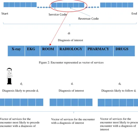
di
Diagnosis of interest
[image:13.612.72.525.189.627.2]X-ray EKG ROOM RADIOLOGY PHARMACY DRUGS
Figure 2: Encounter represented as vector of services
dj di dk
Diagnosis likely to precede di Diagnosis of interest Diagnosis likely to follow di
Figure 3: Vector of services for episode of care
Vector of services for the encounter with a diagnosis of interest
Vector of services for the encounter most likely to precede encounter with a diagnosis of
7
Figure 2 illustrates an encounter represented as a vector of services (mapped by procedural and
revenue codes) provided to a patient. In their study, Zhang et al. [12] clustered encounters,
represented by revenue codes, corresponding to claims associated with a given primary diagnosis.
Figure 3 shows the scope of the proposed methodology. For any patient, the episode of care
comprises services associated with the diagnoses of interest and with the encounters most likely
to precede and follow.
2. Literature Review
Several case studies have confirmed the value of adopting BPs as an effective means of reducing
health care costs. In one such program, The Texas Heart Institute adopted BPs for cardiovascular
surgeries of non-Medicare patients as early as 1984. The associated study showed that the
program’s combined facility and physician’s fees reduced coronary artery bypass costs by 44%
[14]. In 1991, the Health Care Financing Administration (HCFA) initiated the Medicare
Participating Heart Bypass Center Demonstration, in which a single negotiated global price was
paid to hospitals and physicians for all inpatient heart bypass care. As a result, the Government
and beneficiaries saved more than $17 million on bypass surgery in the four participating
institutions [15]. In 2006, the Geisinger Health System ProvenCare bundle payment model was
adopted for coronary artery bypass graft (CABG) procedures. Payments included the cost of
hospitalization and services within 90 days of discharge following surgery [16]. All patients treated
during the one-year period were compared with 137 patients treated in 2005. The results showed
a 16% decrease in length of stay, and mean hospital charges fell by 5.2% [17]. The Health Care
Incentives Improvement Institute implemented a bundled payment model named PROMETHEUS
for twenty-one chronic and acute medical conditions. Pilot sites implementing PROMETHEUS
8
reductions. In a study of 3942 patients undergoing joint replacements between July 2008 and June
2015, Navathe et al. [19] confirmed that a hospital that adopted the PROMETHEUS BP reduced
the cost per episode of care from $26,785 to $21,208, and the length of prolonged hospital stays
decreased by 67.0%. In 2009, Blue Cross Blue Shield of Massachusetts (BCBSMA) introduced
the Alternative Quality Contract (AQC), which combines a fixed per-patient payment with
performance incentive payments to reduce costs and improve health care quality [20]. AQC
enrollees experienced improved quality and lower spending between 2009 and 2013 when
compared with similar populations elsewhere [21].
Among recent implementations of BP models, The Centre for Medicare and Medicaid Innovation
has developed the Bundled Payments for Care Improvement (BPCI) initiative. BPCI proposed four
models for bundling episodes of care, allowing participating hospitals to choose between these. In
Model 1, BPs relate to episodes of care involving inpatient stay in acute care hospitals. In Models
2 and 3, Medicare uses the FFS reimbursement method to make payments to providers for all
services. Total expenditure for an episode is compared against a predetermined BP by CMS. If
total expenditure is below the bundled payment amount, the net profit is shared between CMS and
the awardee; on the other hand, if expenditure exceeds the bundle payment amount, the awardee
has to pay a recoupment amount to CMS. In this instance, awardees are providers that have signed
an agreement with CMS and assume financial liability for episode spending. Model 2 applies to
retrospective acute and acute care episodes, and Model 3 applies only to retrospective
post-acute care. In Model 4, CMS makes a single predetermined bundle payment to the hospital for an
episode of care, covering the cost of all services, physicians and related readmissions, and
9
two phases. By July 1, 2015, BPCI covered 2,115 participating providers [22].
BP implementations have shown promising results. Although very few models have been
implemented, they advance understanding of the feasibility and effect of bundled payments. In the
first place, all of these programs have been implemented in highly integrated systems, such as
academic medical centers or large hospitals, which offers a wide range of services. As such, their
design and outcomes may not be generalizable. Second, characterization of an episode of care is
difficult. In some existing BP models, episodes may be shorter or more extended, as bundled
payments require definition of included and excluded services. Third, pricing of an episode of care
varies significantly, and this may discourage adoption of BPs. Bundled payment implementations
have used different strategies entailing varying levels of financial risk for providers and payers.
An additional challenge is reaching an agreement between payers and providers on a payment
strategy and division of financial risk acceptable to both. Finally, risk adjustment must be properly
defined. Risk adjustment relates to variations in such factors as patient demographics, location,
and severity of illness. This study focuses on episode characterization. There follows a discussion
of the various methodologies proposed to assist episode characterization and subsequent
challenges arising.
A number of studies have based episode of care characterization on changes in resource
consumption. Among these, Mehta et al. [23] monitored changes in resource consumption to
define the duration of an episode of care for diabetic foot ulcers. That study defined the episode of
care as beginning with increased resource consumption; similarly, a decrease in resource
10
one single pre-admission interval and a single post-admission interval to define episodes of care
and determined the duration of the encounter as the aggregated sum of all patient services during
the pre-admission interval and the post-discharge period. To determine such intervals, a 180-day
period (for pre-admission or post-admission) was partitioned into two parts, using a point Tc (T1 <
Tc < T180) such that difference of the mean service count between two partitions [T1,Tc ] and
[Tc,T180] was maximum and the variance in each partition was minimum. Conditions covered in
the study included malignant breast cancer, renal dialysis and caesarean delivery. Schulman et al.
[25] used average weekly charges and the proportion of days incurring charges as markers to define
the beginning and end of an episode of care. Wall et al. [26] defined the beginning and end of an
episode of care in terms of the minimum number of encounters required to constitute an episode
and the length of a clear zone, defined as the time interval between two encounters. Similarly,
Alemi et al. [27] proposed a characterization of episodes of care based on the time interval between
two consecutive diagnoses and their similarity. Cave [28] used a diagnostic cluster in combination
with a fixed time window; claims that fell into the same category within a given time window for
that category were grouped together in the same episode of care; a new episode was created if the
gap between claims exceeded the time window defined for the category. Costs were sensitive to
the duration of the gap between two diagnoses or between two claims. Several other methodologies
have also been used to determine the length of an episode of care, but the actual duration of
episodes of care for any given diagnosis remains uncertain.
Other approaches to episode characterization include rule-based algorithms, which require domain
knowledge and are labor-intensive. Hornbook et al. [29] developed a rule-based algorithm to
define the episode of care for pregnancy. Forthman et al. [30] used episode treatment groups to
11
episodes of care consisting of six pre-specified iterative steps, grouping 31 illnesses into five
generic types of episode. However, as the proposed heuristic is specific to the given condition, it
cannot be adapted for the wider population or for other subsets of patients and conditions.
Construction of a comprehensive set of rules to characterize all episodes of care may prove too
time-consuming.
Data mining techniques have been applied in a variety of health care domains, including episode
characterization, disease classification, and cost prediction. Using a supervised learning approach,
Son et al. [32] clustered claims into episodes that minimized a specific cost function, based on
claims data and imaging reports. In the absence of additional information, such as physicians’
notes and imaging reports, the model performs poorly. Kaur et al. [33] used cases registered to the
California Department of Alcohol and Drug Programs (ADP) to improve drug recovery services,
where k-means and hierarchical clustering techniques were used to show that the likelihood of
substance abuse depends on the patient’s education level, age, and marital status [33]. Jabbar et al.
[34] developed a method for classifying heart disease based on such factors as age, gender, and
obesity, using k-nearest neighbor and genetic algorithms. Lebedev et al. [35] applied random forest
techniques to clinical and magnetic resonance imaging data to detect Alzheimer’s disease. Using
k-nearest neighbor to predict patients’ rehabilitation potential, Zhu et al. [36] showed that the
algorithm performed better than those used in clinical assessment protocols. Using a neural
network, Kuo et al. [37] developed a model to estimate the medical cost of acute hepatitis patients.
Ismael et al. [38] also developed a set of neural network models of hospital charges for acute
coronary syndrome patients and compared their performance. The present study uses both
12
multi-class classification) to predict treatment cost by cluster, which requires better cluster
characterization and better cost estimation per cluster.
To address some of the challenges in characterizing episode of care, Zhang et al. [12] proposed a
methodology to cluster encounters on the basis of procedural patterns within each encounter. They
used spectral clustering [13] to group inpatient encounters associated with a given primary
diagnosis and then analyzed the service and cost patterns of the resulting clusters. However, they
failed to directly consider the impact of co‐morbidities. To take account of this effect, we have extended Zhang et al. [12] by analyzing the effect of including services for encounters most likely
to precede and follow the encounter of interest.
3. Methodology
For clustering based on procedural and non-procedural information, encounters are represented as
n-dimensional vectors. Encounters involving services associated with a primary diagnosis of
interest were selected, along with encounters most likely to immediately precede and follow that
encounter, as identified through correlation and directionality analyses. Spectral clustering was
used to group these encounters, assigning each encounter to a given cluster-id. The output of the
first clustering step was used as an input to a secondary classification step, employing supervised
learning algorithms such as naïve Bayes, support vector machine, k-nearest neighbors, boosting,
random forest, and feed-forward neural network. Different combinations of independent variables
were used to train the model, using the supervised learning methods mentioned above and
comparing them using specific performance metrics. Cost variation was analyzed for each cluster
13
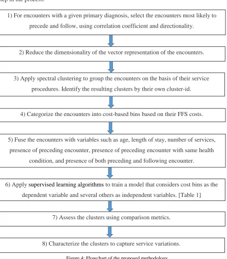
Figure 4 provides an overview of this methodology, followed by a detailed explanation of each
[image:20.612.76.522.108.617.2]step in the process.
Figure 4: Flowchart of the proposed methodology
1) For encounters with a given primary diagnosis, select the encounters most likely to
precede and follow, using correlation coefficient and directionality.
2) Reduce the dimensionality of the vector representation of the encounters.
3) Apply spectral clustering to group the encounters on the basis of their service
procedures. Identify the resulting clusters by their own cluster-id.
4) Categorize the encounters into cost-based bins based on their FFS costs.
6) Apply supervised learning algorithms to train a model that considers cost bins as the
dependent variable and several others as independent variables. [Table 1]
7) Assess the clusters using comparison metrics.
8) Characterize the clusters to capture service variations.
5) Fuse the encounters with variables such as age, length of stay, number of services,
presence of preceding encounter, presence of preceding encounter with same health
14
3.1 Selecting encounters
3.1.1 (Correlation coefficient) Selecting encounters most likely to precede and follow an encounter of interest
To determine the encounter immediately preceding and following the encounter of interest, we
rely on correlation and directionality analysis similar to the approach used by Hidalgo et al. [39]
in developing a Phenotypic Disease Network (PDN) to study comorbidity associations between
diseases. We analyze the likelihood of occurrence of any two primary diagnoses in consecutive
encounters across all patients.
To study the strength of the relationship between two diagnoses, we rely on the correlation
coefficient between two diagnoses as in (1). We select encounters whose correlation coefficients
are positive and significant. Let ϕi,j be a correlation coefficient, as defined in (1).
𝜙𝜙
𝑖𝑖,𝑗𝑗=
𝐶𝐶𝑖𝑖𝑖𝑖𝑁𝑁−𝑃𝑃𝑖𝑖𝑃𝑃𝑖𝑖�𝑃𝑃𝑖𝑖𝑃𝑃𝑖𝑖(𝑁𝑁−𝑃𝑃𝑖𝑖)�𝑁𝑁−𝑃𝑃𝑖𝑖�
(1),
where
Cijis the number of patients affected by both diagnoses (i and j);
N is the total number of patients; and
Pi is the number of patients affected by ith diagnosis.
Once all 𝜙𝜙𝑖𝑖,𝑗𝑗 have been identified, we establish statistical significance, using a t-test at 95 %
confidence level, to evaluate whether ti,j> t0.975, as defined in (2).
𝑡𝑡
𝑖𝑖,𝑗𝑗=
𝜙𝜙𝑖𝑖,𝑖𝑖√𝑛𝑛−2�1−𝜙𝜙𝑖𝑖2,𝑖𝑖
15
where n is the maximum number of patients between Pi and Pj (max (Pi,Pj)).
A high correlation value indicates a strong relationship between diagnoses.
3.1.2 Directionality
The correlation coefficient provides information about the relationship between two diagnoses but
says nothing about any causal association between them. The notion of directionality is needed to
understand the progression and relationship of the diagnoses. Positive directionality between
diseases i and j implies that a patient with ith diagnosis is most likely to be followed by a jth
diagnosis. Hidalgo et al. [41] used directionality between two connected diseases to design a PDN
to analyze which diagnoses were most likely to follow other diagnoses.
The strength of the relationship is calculated using directionality λi→j between two diagnoses i and
j as given in (3).
λ
i→j=log
10�
li→j
lj→i
�
(3),where
li→j =(Li→j+1)/Pi;
Li→jis the number of times diagnosis i was diagnosed before diagnosis j ;
Cijis the number of patients affected by both diagnoses (i and j); and
Pi is the number of patients affected by ith diagnosis.
When computing Li→j, we disregard those cases where both diagnoses were diagnosed in the same
16
diagnosis and negative if a diagnosis tends to follow another [39]. We select all pairs of diagnoses
with directionality above a minimum threshold, to be varied from 0.25 to 3.75.
The sample of encounters containing services for the diagnosis of interest and the preceding and
following encounters is larger than that used by Zhang et al. [12] for the same diagnoses of interest.
3.2 Reducing the dimensionality of the encounter vector’s representation
We also used the dimensionality reduction technique proposed by Zhang et al. [12] for encounters
represented as a vector of services, applying spectral clustering. Medical and clinical services are
encoded in multiple systems, including Current Procedural Terminology (CPT) codes as used by
the American Medical Association (AMA); Healthcare Common Procedure Coding System
(HCPCS) codes as used by CMS; Primary Procedure Codes as used by the National Centre for
Health Statistics of the U.S. Public Health Service; and Revenue Codes as used by the National
Uniform Billing Committee. There are over 9,000 CPT/HCPCS codes, many of which differ very
little. To reduce the dimensionality of these codes and to generate clusters with high cost
differences for clinical services, we adopt the dimensionality reduction approach proposed by
Zhang et al. [12], using Clinical Classifications Software for Services and Procedures (Agency for
Healthcare Research and Quality 2017) to synthesize all CPT/HCPCS codes into 244 categories.
When using revenue codes, the authors use their first two digits, which refer to hospital service
categories.
To characterize an episode of care, the encounter associated with the episode is represented as the
17
diagnosis. Each dimension represents the presence or absence of the services by a binary indicator,
depending on whether or not the service was provided to a patient during the encounter. We do
not include service frequencies in the vector, focusing on the procedural heterogeneity of services
for the given diagnosed condition rather than on differences in the magnitude of services delivered.
3.3 Applying spectral clustering to group the encounters based on service procedures
Once all encounters are collected and represented as a vector of services, spectral clustering as
proposed by Kannan et al. [13] will be used to determine a group of encounters with maximum
similarity within the same cluster and minimum similarity among encounters of different clusters.
After summarizing the services, a clustering algorithm is used to group encounters on the basis of
services provided. Based on revenue and procedure codes, we cluster those encounters involving
similar services.
Similarity between two encounters i and j (represented as service vectors xiand xj) is measured
using cosine similarity aijas in (4).
𝑎𝑎
𝑖𝑖𝑗𝑗=
(𝑥𝑥𝑖𝑖)∗(𝑥𝑥𝑖𝑖)||𝑥𝑥𝑖𝑖||∗||𝑥𝑥𝑖𝑖|| (4),
where
0 <= aij <= 1
The cosine similarity metric is commonly used with sparse binary data, offering more subtlety than
a Euclidean distance metric for high-dimensional data. To perform the spectral clustering, we
construct the similarity matrix A = [aij]. We can visualize our data in the form of a graph, where
18
should yield high similarity within clusters, as measured by high conductance and low similarities
between sub-graphs, expressed by intercluster weights. The spectral clustering algorithm [13]
identifies clusters by applying optimization to the (α, ε) measure, where α reflects the compactness
of each cluster and ε measures the differences between clusters. This bi-criteria measure is robust,
as it seeks to optimize both measures simultaneously, unlike other approaches such as k-center or
k-median, which focus on the optimization of a single measure.
The number of clusters is controlled by a tuneable parameter that takes account of both (α, ε)
criteria. To study the major clinical service pattern while characterizing episodes of care, we focus
on generating large clusters. Once clustering has been performed for a given (α, ε), each encounter
is assigned a cluster-id. This information is used in a classification step that relies on the use of
cost-based bins.
3.4 Categorizing encounters into cost-based bins
The cluster-based bundle payment assumes that treatment costs should be the same for all
encounters in any given cluster, enabling the division of encounters on the basis of FFS total cost.
The sample of encounters used in the first clustering step are classified into cost categories based
on their FFS total costs in order to enhance cluster quality and to regenerate new clusters with less
heterogeneous costs. Encounters are divided into bins on the basis of cost such that the number of
bins generated is equal to the number of clusters generated from spectral clustering. As each bin
corresponds to a group of clusters with similar total FFS cost, each encounter in a given cluster
should be assigned the same bundle payment amount. We first rank all encounters by FFS total
19
in each bin is approximately the same [40]. Consequently, each bin may contain a different number
of encounters. Once categorization has been performed, each encounter is assigned a cost bin label,
which serves as the dependent variable for the models in section 3.5.
3.5 Applying supervised classification algorithms to train the model
We further enrich the encounter data set so that the encounters contain information about their
cluster membership (from the spectral clustering step), with independent variables such as length
of stay, cluster-id, number of services per encounter, preceding encounter cost, presence of
preceding encounter, presence of preceding encounter with same primary health condition,
presence of preceding and following encounters as described in Table 1, and categorical cost bin
labels (from the previous cost bins categorization step). We use different possible combinations of
the independent variables described in Table 1 to predict the cost bin label, using supervised
classification algorithms with k-fold stratified sampling. The selected classification algorithms are
naïve Bayes, support vector machines, k-nearest neighbors, random forest, boosting, and
feed-forward-neural network.
The presence of continuous variables like length of stay makes it difficult to implement spectral
clustering for the classification step. As a result, we proceed with supervised classification
algorithms for the second classification step. Once the models have been defined, we compare the
models, using metrics of comparison that enable assessment of correctness in predicting the
20
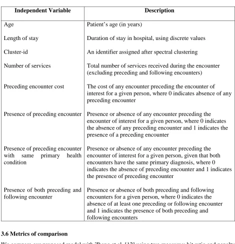
Table 1: Description of independent variables used during exploration of supervised classification algorithms
Independent Variable Description
Age
Length of stay
Cluster-id
Number of services
Preceding encounter cost
Presence of preceding encounter
Presence of preceding encounter with same primary health condition
Presence of both preceding and following encounter
Patient’s age (in years)
Duration of stay in hospital, using discrete values
An identifier assigned after spectral clustering
Total number of services received during the encounter (excluding preceding and following encounters)
The cost of any encounter preceding the encounter of
interest for a given person, where 0 indicates absence of any preceding encounter
Presence or absence of any encounter preceding the encounter of interest for a given person, where 0 indicates the absence of any preceding encounter and 1 indicates the presence of a preceding encounter
Presence or absence of any encounter preceding the encounter of interest for a given person, given that both encounters have the same primary diagnosis, where 0 indicates the absence of preceding encounter and 1 indicates the presence of preceding encounter
Presence or absence of both preceding and following encounters for a given person, where 0 indicates the absence of at least one preceding or following encounter and 1 indicates the presence of both preceding and following encounters
3.6 Metrics of comparison
We compare our proposed model with Zhang et al. [12] using two measures: hit ratio and penalty
error, as used by Bertsimas et al. [40].
(1) Hit Ratio: This corresponds to the percentage of encounters with correct cost bin prediction.
This can also be referred to as the accuracy of the model.
(2) Penalty Error: This corresponds to the penalty of underestimation and overestimation. While
21
error assigns different costs to underestimation and overestimation. The error cost of
underestimation is higher than for overestimation and is set as twice the penalty of overestimation
due to the chance of loss to the providers [40]. The penalty error is defined as an average penalty
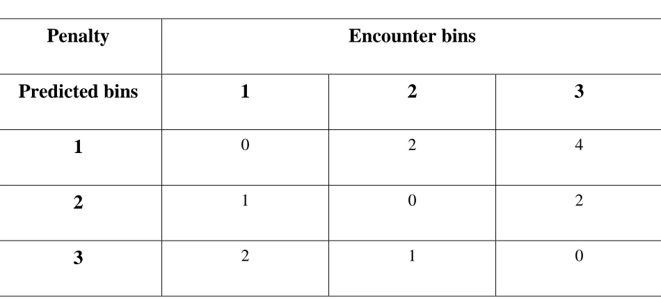
(i.e., penalty per encounter). Table 2 shows the penalty table scheme for the 3-bins system.
Encounter bins are arranged in order of cost (first as least expensive, last as most expensive). A
predicted bin of 2 with actual bin of 1 implies underestimation, attracting a penalty of 1. On the
other hand, a predicted bin of 2 and actual bin of 1 implies overestimation, attracting a penalty of
[image:28.612.76.551.357.572.2]1.
Table 2: Penalty table
Penalty
Encounter bins
Predicted bins
1
2
3
1
0 2 42
1 0 23
2 1 0The model with lowest penalty error and highest hit ratio is selected. Finally, we will analyze the
22
3.7 Characterizing the cluster
Various cluster features such as encounter costs and their variations were analyzed by Zhang et al.
[12], using coverage rate to assess the cluster’s services variation. Coverage rate is used to capture
homogenous procedural patterns among clusters; it is defined as the fraction derived from
occurrences of the procedures in a set of services R and occurrences of all procedures for patients
within the cluster:
𝐶𝐶𝐶𝐶𝐶𝐶𝐶𝐶𝐶𝐶𝑎𝑎𝐶𝐶𝐶𝐶
𝑅𝑅𝑎𝑎𝑡𝑡𝐶𝐶
𝑗𝑗=
∑𝑖𝑖𝜀𝜀𝑅𝑅 𝑟𝑟𝑖𝑖𝑖𝑖∑𝑖𝑖𝜀𝜀𝑅𝑅 𝑟𝑟𝑖𝑖𝑖𝑖+∑𝑖𝑖∉𝑅𝑅 𝑝𝑝𝑘𝑘𝑖𝑖 (5),
where
R is defined as set of services with more than 10% representation in at least one of
the clusters;
rij is the ratio of patients in cluster j receiving service i; and
pkj is the ratio of patients in cluster j receiving service k, which is not in R.
A higher coverage rate indicates that a large portion of the procedural variation is captured by the
representation. Additionally, we used the coefficient of variation (CV) to analyze payment
variations for each cluster, as defined in (6).
𝐶𝐶𝐶𝐶
𝑗𝑗=
𝑃𝑃𝑃𝑃𝑃𝑃𝑃𝑃𝑃𝑃𝑛𝑛𝑡𝑡 ′𝑠𝑠𝑆𝑆𝑆𝑆𝑖𝑖23
Patients in a cluster share common services and specialist examinations, which influences cost per
hospitalization. Low variation in costs within a cluster would imply that the homogeneity of
procedures or services is also reflected in the costs. Costs within each cluster can assist accurate
prediction of future cases involving similar conditions. The coefficient of variation (CV) is defined
as the fraction derived from the standard deviation and average cost of any resulting cluster j.
3.8 Analyzing cluster quality
To compare clusters that differ from each other in terms of distribution of features such as gender,
age, insurance type, length of stay, and mean cost per encounter, we conduct a pairwise comparison
of the resulting clusters based on the mean for each feature, using Tukey’s honest significant
differences (HSD) test as in Zhang [12] to facilitate comparison with Zhang’s approach.
We also apply the Bonferroni correction to control any increment in Type I error. The threshold
for Type I error is set at 𝛼𝛼 = 0.05, and we reject every individual null hypothesis at level
𝛼𝛼
sig.𝛼𝛼
𝑁𝑁(𝑁𝑁−1)/2
(7),
where N is the number of clusters.
The set of encounters generated by the included encounters will be a superset of the set of
encounters generated by Zhang et al. [12]. The comparison with Zhang’s approach involves
comparing the underpayment and overpayment cost variation for encounters common to both
approaches. The effect of directionality and controlling parameter (α) used in clustering will be
examined below.
24
4. Data
The data used here comprise de-identified and Health Insurance Portability and Accountability Act
of 1996 (HIPAA) compliant insurance claims records of 1.6 million residents of nine counties in
Upstate NY, generated between 2007 and 2014. The data set contains 334 million claim records,
containing information related to health care services that include inpatient, outpatient, and
pharmacy procedures. In the data, an encounter refers to the set of services sharing a primary
diagnosis by ICD-09 or ICD-10 code, encompassing all services from a patient’s first visit to a
health care provider to discharge or last visit. An individual can have more than one encounter.
For each encounter, the information includes start date, end date, primary diagnosis code,
secondary diagnosis code, claim type, place of encounter, and total encounter cost. This can be
viewed as a high-dimensional vector, where each dimension represents a feature of the encounter.
The primary and secondary diagnosis codes represent the medical conditions for which the patient
is treated. To protect patient identity, all service dates were masked by a random shift in reported
dates between [-15, +15] while preserving the order of services. Dates of encounters were
randomized by Finger FLHSA, making it impossible to trace the patient.
Any service involving shifted dates falling outside the given study period were excluded. Each
patient was assigned a unique member identification number (for research purposes only), and
each can be associated with multiple encounters. This patient id does not correspond to any
insurance or hospital identifier. The revenue and procedure codes map onto services and resources
consumed during a given encounter. While information such as age and gender is also available,
information about very young and very elderly individuals has been excluded from the database
25
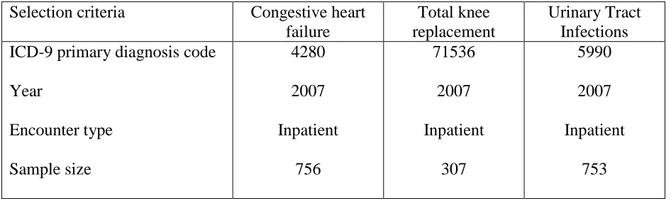
Table 3: Summary description of the dataset
Selection criteria Congestive heart
failure
Total knee replacement
Urinary Tract Infections ICD-9 primary diagnosis code
Year Encounter type Sample size 4280 2007 Inpatient 756 71536 2007 Inpatient 307 5990 2007 Inpatient 753
5. Analysis
5.1 Congestive heart failure (CHF) study
Using the proposed methodology, we implemented the clustering algorithm for inpatients with
CHF. The sample size was determined by threshold directionality; high-value thresholds result in
low sample sizes, as they include only encounters with diagnoses that are more likely to precede
or follow the given diagnosis. The sample size with directionality 0.25 is 756 and the sample size
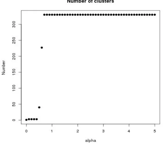
with directionality 3.75 is 607. The number of clusters was determined by the parameter α and is
also affected by directionality as shown in Figure 5 (for directionality 3.75) and Figure 6 (for
directionality 0.25). The number of clusters is low for lower values of α and increases as α
increases. A higher number of clusters results in a smaller number of encounters within each
individual cluster generated, hindering interpretation of the clusters. We set the tuning parameter
α at 0.4, resulting in 3 clusters. Inter-cluster and within-cluster similarity confirms that the
26
Figure 5: Number of clusters versus α for directionality 3.75
[image:33.612.150.446.409.659.2]27
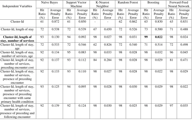
The three generated clusters have sample sizes of 385, 264, and 107. Based on the results shown
in Table 4, the boosting model with cluster-id, length of stay, and number of services as
independent variables has a high hit ratio and low average penalty error. Table 5 shows the
standard deviation of underpayments and overpayments to the provider (hospitals), where a single
payment is made to hospitals for each encounter, based on the mean total FFS cost for each cluster
and according to cluster membership. Using the proposed methodology, total standard deviation
28
Table 4: Results of CHF obtained using supervised classification algorithms
Independent Variables
Naïve Bayes Support Vector
Machine
K-Nearest Neighbor
Random Forest Boosting Forward-Feed
Neural Network Hit Ratio (%) Average Penalty Error Hit Ratio (%) Average Penalty Error Hit Ratio (%) Average Penalty Error Hit Ratio (%) Average Penalty Error Hit Ratio (%) Average Penalty Error Hit Ratio (%) Average Penalty Error
Cluster-Id 61 0.872 61 0.850 - - 62 0.862 63 0.830 63 0.831
Cluster-Id, length of stay 72 0.538 72 0.539 67 0.650 72 0.526 73 0.500 71 0.488
Cluster-Id, length of stay, number of services
93 0.130 94 0.092 98 0.027 98 0.031 99 0.022 98 0.024
Cluster-Id, length of stay, age
72 0.533 72 0.546 62 0.826 72 0.540 71 0.514 72 0.498
Cluster-Id, length of stay, number of services, age
92 0.134 95 0.083 98 0.033 98 0.028 98 0.032 96 0.045
Cluster-Id, length of stay, number of services, preceding encounter cost
92 0.137 93 0.112 84 0.284 98 0.028 98 0.029 81 0.471
Cluster-Id, length of stay, number of services, presence of preceding
encounter
92 0.133 93 0.110 98 0.027 98 0.028 98 0.022 98 0.029
Cluster-Id, length of stay, number of services, presence of preceding
encounter with same primary health condition
93 0.125 94 0.095 98 0.028 98 0.030 98 0.029 98 0.022
Cluster-Id, length of stay, number of services, presence of preceding and
following encounter
29
As CHF is a medically complex condition, the three clusters generated from the proposed
methodology have low coverage rates (83.1%, 82.1%, and 82.9 % for clusters 1, 2, and 3,
respectively). The resulting cluster service representation is shown in Figure 7.
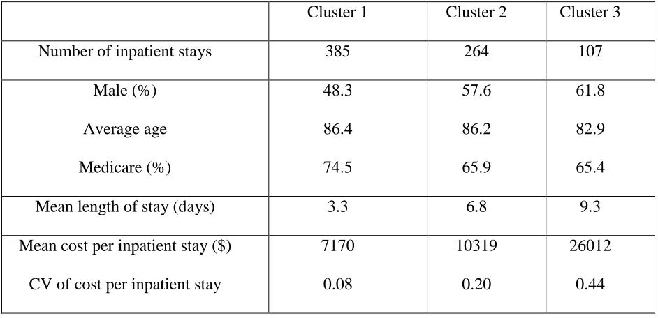
We further investigated differences between the clusters on the basis of non-procedural cluster
features such as insurance type, age, gender, length of stay, and cost level and variation. The results
for all three clusters are shown in Table 5. Patients in the cluster with low average age tend to be
less likely to be on Medicare. The differences between cluster 2 and other clusters are statistically
significant; results of statistical testing for non-procedural features are shown in Table 6. As cluster
1 is characterized by low length of stay, inpatient cost is low. Figure 8 shows the distribution of
[image:36.612.71.542.396.624.2]total cost per inpatient stay within each cluster.
Table 5: Non-procedural characteristics of CHF clusters
Cluster 1 Cluster 2 Cluster 3
Number of inpatient stays 385 264 107
Male (%)
Average age
Medicare (%)
48.3
86.4
74.5
57.6
86.2
65.9
61.8
82.9
65.4
Mean length of stay (days) 3.3 6.8 9.3
Mean cost per inpatient stay ($)
CV of cost per inpatient stay
7170
0.08
10319
0.20
26012
30
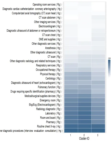
Figure 7: Representation of three CHF clusters.
Each row represents a service. The darkness level of each cell indicates the percentage of patients in the cluster (column) who received the service (row). Following each service name, “Rg” stands for hospital services; “Hg”
31
Table 6: Results of hypothesis testing
(Tukey’s HSD testing for nonprocedural features) among CHF clusters at family-level confidence level = 0.05. NS stands for non-significant results of comparisons. *, **, *** denote a significance level of 5%, 1%, and 0.1%,
respectively
C1 and C2 C2 and C3 C1 and C3
Male (%)
Average age
Medicare (%)
***
NS
***
**
**
NS
***
**
***
Mean length of stay (days) *** *** ***
Mean cost per inpatient stay ($) *** *** ***
[image:38.612.127.456.343.628.2]
32
The generated clusters also exhibit significant differences for non-procedural features as well,
supporting our classification process in characterizing the episode of care. The generated clusters
are compared with those generated using Zhang et al.’s [12] method for the same data based on
financial risk. The composition and distribution of clusters differ from Zhang’s, and it is difficult
to exactly match the clusters in our methodology with any particular cluster in Zhang’s
methodology. The methodology proposed here also resulted in reduction of the risk associated
[image:39.612.56.560.332.588.2]with overpayment/underpayment as shown in Table 7.
Table 7: Standard deviation of underpayment/ overpayment for CHF with respect to mean total FFS for encounters by cluster
Zhang’s Methodology Proposed Methodology
Cluster
1
Cluster
2
Cluster
3
Total Cluster
1
Cluster
2
Cluster
3
Total
Sample size 430 26 50 506 282 162 62 506
Mean cost of encounters ($)
8705 13100 25217 10936 7182 10345 25095 10936
Standard deviation of underpayment or overpayment value ($)
33
5.2 Total knee replacement (TKR) study
The sample size for directionality 0.25 is 307, and the sample size for directionality 3.75 is 295.
Proceeding with 0.25 directionality, we used clusters with 25 or more inpatient stays. The three
large generated clusters used here contain 71, 73, and 146 inpatient stays, respectively.
Based on the results in Table 8, the random forest model including cluster-id, length of stay, and
age show better performance. Table 9 shows the standard deviation of underpayments and
overpayments to the provider (hospitals) incurred by adoption of a cluster-based bundle payment.
The total variation/standard deviation in the proposed methodology is again lower in comparison
to the variation in Zhang’s methodology.
34
Table 8: Results of TKR obtained using supervised classification algorithms
Independent Variables
Naïve Bayes Support Vector
Machine
K-Nearest Neighbor
Random Forest Boosting Forward-Feed
Neural Network Hit Ratio (%) Average Penalty Error Hit Ratio (%) Average Penalty Error Hit Ratio (%) Average Penalty Error Hit Ratio (%) Average Penalty Error Hit Ratio (%) Average Penalty Error Hit Ratio (%) Average Penalty Error
Cluster-Id 46 1.228 48 1.22 - - 48 1.163 46 1.197 47 1.207
Cluster-Id, length of stay 43 1.263 47 1.244 46 1.218 48 1.130 46 1.197 46 1.174
Cluster-Id, length of stay, number of services
41 1.244 47 1.269 44 1.193 46 1.193 46 1.192 47 1.116
Cluster-Id, length of stay, age
43 1.049 48 1.207 46 1.106 52 0.948 49 1.048 41 1.521
Cluster-Id, length of stay, number of services, age
42 1.052 48 1.190 43 1.254 44 1.133 47 1.113 40 1.703
Cluster-Id, length of stay, number of services, preceding encounter cost
37 1.214 47 1.260 45 1.177 44 1.165 43 1.221 45 1.177
Cluster-Id, length of stay, count of services, presence of preceding
encounter
37 1.181 46 1.301 45 1.195 42 1.249 45 1.209 43 1.172
Cluster-Id, length of stay, count of services, presence of preceding
encounter with same primary health condition
37 1.181 41 1.650 45 1.186 44 1.184 45 1.212 47 1.137
Cluster-Id, length of stay, count of services, presence of preceding and
following encounter
35
Because TKR is a medically less complex condition than CHF, the three clusters generated using
the proposed methodology have high coverage rates (95.1%, 94.1%, and 93.6% for clusters 1, 2
and 3 respectively). The resulting cluster service representation is shown in Figure 9. Standard
procedure knee replacement surgery is present in all three clusters.
The results for non-procedural characteristics for all three clusters are shown in Table 9. Clusters
with low mean length of stay tend to be low-cost. Cluster 1 has low length of stay and therefore
low inpatient cost. Figure 10 shows the distribution of total cost per inpatient stay within each
cluster. The results of statistical testing for non-procedural features are shown in Table 10. Clusters
[image:42.612.72.542.374.600.2]2 and 3 show no statistical differences.
Table 9: Non-procedural characteristics of TKR clusters
Cluster 1 Cluster 2 Cluster 3
Number of inpatient stays 109 148 33
Male (%)
Average age
Medicare (%)
44.0
83.9
86.2
33.8
78.5
41.9
48.5
71.9
9.1
Mean length of stay (days) 3.2 3.3 4.1
Mean cost per inpatient stay ($)
CV of cost per inpatient stay
13623
0.15
15174
0.15
15929
36
Figure 9: Representation of three TKR clusters.
Each row represents a service. The darkness level of each cell indicates the percentage of patients in the cluster (column) who received the service (row). Following each service name, “Rg” stands for hospital services; “Hg”
37
Table 10: Results of hypothesis testing
(Tukey’s HSD testing for nonprocedural features) among TKR clusters at family-level confidence level = 0.05. NS stands for non-significant results of comparisons. *, **, *** denote a significance level of 5%, 1%, and 0.1%,
respectively
C1 and C2 C2 and C3 C1 and C3
Male (%)
Average Age
Medicare (%)
***
***
***
***
***
***
NS
***
***
Mean length of stay (days) NS *** ***
Mean cost per inpatient stay($) *** *** NS
[image:44.612.85.491.342.650.2]38
Table 11: Standard deviation of underpayment/ overpayment for TKR with respect to mean total FFS for encounters by cluster
Zhang’s Methodology Proposed Methodology
Cluster
1
Cluster
2
Cluster
3
Total Cluster
1
Cluster
2
Cluster
3
Total
Size 72 73 145 290 109 148 33 290
Mean cost of encounters ($)
13932 14326 15215 14677 13623 15174 15929 14677
Standard deviation of underpayment or overpayment value ($)
1557 1149 1904 1689 1207 1910 1724 1668
5.3 Urinary Tract Infections (UTI) Study
The sample size with UTI health condition for directionality 0.25 is 753. The six large clusters
generated with more than 25 inpatient stays, have 28, 53, 54, 56, 179 and 351 inpatient stays.
Based on the results shown in Table 12, the boosting model with Cluster-Id and length of stay as
predictors has better performance. Table 16 shows the standard deviation of underpayments and
39
Table 12: Results of UTI obtained using supervised classification algorithms
Independent Variables
Naïve Bayes Support Vector
Machine
K-Nearest Neighbor
Random Forest Boosting Forward-Feed
Neural Network Hit Ratio (%) Average Penalty Error Hit Ratio (%) Average Penalty Error Hit Ratio (%) Average Penalty Error Hit Ratio (%) Average Penalty Error Hit Ratio (%) Average Penalty Error Hit Ratio (%) Average Penalty Error
Cluster-Id 20 3.666 21 3.880 - - 19 3.616 22 3.947 20 3.766
Cluster-Id, length of stay
26 2.167 28 2.759 31 2.063 30 2.267 35 2.057 30 2.403
Cluster-Id, length of stay, count of services
25 2.224 29 2.755 26 2.196 27 2.252 30 2.161 30 2.258
Cluster-Id, length of stay, age
29 2.091 30 2.809 27 2.197 29 2.189 31 2.029 30 2.265
Cluster-Id, length of stay, count of services, age
28 2.096 29 2.914 23 2.382 27 2.081 31 2.080 29 2.186
Cluster-Id, length of stay, count of services, preceding encounter cost
25 2.391 27 2.838 28 2.184 24 2.201 31 2.165 27 2.319
Cluster-Id, length of stay, count of services, presence of preceding
encounter
25 2.455 27 2.856 26 2.200 25 2.191 31 2.169 29 2.151
Cluster-Id, length of stay, count of services, presence of preceding
encounter with same primary health condition
25 2.455 27 2.956 27 2.184 24 2.223 30 2.163 29 2.236
Cluster-Id, length of stay, count of services, presence of preceding and
following encounter
40
Six UTI clusters were generated from the proposed methodology. The resulting clusters’ service
representation is shown in Figure 11. The clusters with low mean length of stay tend to have low
cost. Cluster 1 has low length of stay and thus low inpatient cost. Figure 12 shows the distribution
[image:47.612.53.551.230.597.2]of the total cost per inpatient stay within each cluster.
Table 13: Non-procedural characteristics of UTI clusters
Cluster 1 Cluster 2 Cluster 3 Cluster 4 Cluster 5 Cluster 6 Number of inpatient stays
252 108 150 23 132 56
Male (%) Average Age Medicare (%) 30.2 79.2 51.9 32.4 78.8 60.2 31.3 86.4 72.7 17.4 83.5 34.8 35.6 87.9 73.5 28.6 86.7 69.6
Mean length of
stay (days)
2.0 2.7 4.5 4.5 7.4 19.8
Mean cost per
inpatient stay($)
CV of cost per
41
Figure 11: Representation of six UTI clusters.
Each row represents a service. The level of darkness in each cell indicates the percentage of patients in the cluster (column) who receive the service (row). Following each service name, “Rg” stands for hospital services; “Hg”
42
Table 14: Results of hypothesis testing
(Tukey’s HSD testing for nonprocedural features) among UTI clusters at family-level confidence level = 0.05. NS stands for non significant results of comparisons. *, **, *** denote a significance level of 5%, 1%, and 0.1%,
respectively
Male
(%)
Average
Age
Medicare
(%)
Mean of length of stay
(days)
Mean cost of per
inpatient stay($)
C1 and C2 NS NS ** NS NS
C1 and C3 NS *** *** *** NS
C1 and C4 *** *** *** NS NS
C1 and C5 NS *** *** *** ***
C1 and C6 NS *** ** *** ***
C2 and C3 NS * * NS NS
C2 and C4 *** *** *** NS NS
C2 and C5 NS * * *** ***
C2 and C6 *** * NS *** ***
C3 and C4 *** *** *** NS NS
C3 and C5 NS NS NS *** *
C3 and C6 * NS * *** ***
C4 and C5 *** *** *** NS NS
C4 and C6 *** *** ** *** ***
43
44
Table 15: Standard Deviation of Underpayment/ Overpayment for UTI with respect to the mean total FFS for encounters in cluster (Zhang’s methodology)
Table 16: Standard Deviation of Underpayment/ Overpayment for UTI with respect to the mean total FFS for encounters in cluster (Proposed methodology)
Proposed Methodology Cluster 1 Cluster 2 Cluster 3 Cluster 4 Cluster 5 Cluster 6 Total
Size 250 108 148 22 130 55 713
Mean Encounters’ cost ($) 6518 6664 7247 7102 8167 12020 7440
Standard deviation of Underpayment/
Overpayment value ($)
634 757 1294 622 2969 4689 2167
Zhang’s Methodology Cluster 1 Cluster 2 Cluster 3 Cluster 4 Cluster 5 Cluster 6 Total
Size 50 54 27 350 54 178 713
Mean Encounters’ cost ($) 7085 7207 7263 7815 7823 7885 7442
Standard deviation of Underpayment/
Overpayment value ($)
[image:51.612.66.563.419.666.2]45
6. Conclusion
The cluster-based bundle payments methodology is valuable in accelerating implementation of
bundle payments and represents a valid alternative to other BP methods. As well as providing the
structure for episode characterization, this automated process can also be generalized across other
conditions, making implementation easy. One of the merits of cluster-based bundle payment over
other methods of episode characterization is that it can be modified according to the patient
population, taking account of the different practices adopted by providers. In turn, providers can
use their own patient data to define the bundle in characterizing the episode of care; in other words,
clustering does not rely on clinical knowledge.
The cluster-based bundled payment system reduces the financial risk for providers and payers as
compared to single-value bundle payment. By modifying Zhang’s cluster-based bundled payment
approach, our cluster-based methodology incurs the same expected expenditures but reduces the
financial risk associated with underpayment and overpayment. This yielded a substantial reduction
in financial risk for slightly less complex conditions such as TKR, as well as for more complex
conditions such as CHF. This reduced financial risk further facilitates adoption of cluster- based
bundle payment.
One of the main challenges for episode characterization is the identification of comorbidities and
different health conditions among patients. Identification of any previous health condition is also
important, as this may affect treatment expenses and financial risk, so hindering adoption of bundle
payment. Our data-driven approach helps in characterizing the episode of care and retrieving a
46
with non-procedural information, our method incorporates comorbidity association, which
improves episode characterization and provides clusters with less cost variation. This payment
scheme can be applied across a wide range of diagnoses and has the potential to further reduce
risk.
In comparing the proposed methodology with Zhang’s methodology, one of the challenges is the
determination of performance metrics. The two methodologies employ a different set of encounters
for the same health condition, although many were common to both. Our study has a larger sample
size, and some of the patients who were assigned to large clusters in one methodology may have
been assigned to smaller renamed clusters in the other methodology. For that reason, the
comparison considered only the common encounters, which may affect our results and
performance metrics. As the comparison using coverage rate showed mixed results, the final
comparison used associated financial risk.
The present study focused only on inpatient data and on three conditions for a single year at the
same hospital, and the effects of including outpatient data, more hospitals, and more years of data
should be explored. This may result in higher financial risks, and health comorbidities and
significant previous health conditions may also vary across years and hospitals. Future work might
use different coding procedures or weighting criteria to include all patients removed in our study.
A number of patients were dropped from our study because they did not belong to any of the large
47
This study presents a novel approach to episode characterization based on a two-step methodology
of clustering followed by classification. The study is unique in including type of clinical and
physician services provided to patients, along with past health condition and evaluation criteria.
This may contribute to a more robust system with better episode characterization and correct cost
48