A Comparative Study on the Performance of Wireless Sensor Networks
Lin Zou
Zhongwei Zhang
Department of Mathematics and Computing
University of Southern Queensland
Toowoomba, QLD, Australia
[email protected]
[email protected]
Abstract
To increase the lifetime of the sensor networks, a recog-nized method is to switch off/on some sensor nodes between “sleep” and “activity” mode in order to save the energy. The performance metrics of an individual node can be cal-culated by using its DTMC model, the theoretical results include the average number of data units generated in a time slotλE, the sensor throughputT, the average buffer occupancy ¯B.
In our research, we have implemented a wireless sensor network on NS2 in which the sensors nodes can be either in sleep or activity modes. Our simulations have produced the experiment results of performance metrics. By compar-ing the experiment results with the theoretical results, we demonstrate the DTMC model is able to accurately describe the behavior dynamics of a sensor node.
1
Introduction
Because sensor nodes usually are so small in size that may be used conveniently in some place, where wired net-work can’t reach or too expensive to install. The sensor nodes are powered by battery which has a limited energy resource. Furthermore, the battery is usually difficult to replace or recharge as the sensor nodes are used in some special fields. As a result, when a sensor node exhausts its power, it will stop its functions. Because of this, the network topology has been changed and the sensor net-work’s capability including sensing phenomenon, informa-tion generainforma-tion and routing data might be degraded. Many researches strive to reduce the energy consumption [3, 4, 5], etc. For instance, a research has introduced to sleep mode to the sensor node which save some energy while the sensor nodes are idle [18].
In this paper, we look at the dynamics of sensor nodes while sensor node states transit from one to another. The rest of this paper is organized as follows. The model of
analyzing the performance of sensor nodes is introduced in Section 2. Simulation environment of NS2 and experiment results are shown in Section 3. We give conclusion and fu-ture work in Section 4.
2
Using Markov Chain to Represent Sensor
Node Dynamics
2.1
Sensor node states
Each sensor is characterized by two operational states: activity and sleep. In activity state the node is full work-load, while in sleep state it cannot take part in the network activity; thus, the network topology will be changed while nodes enter or exit the sleep state.
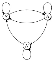
Based on the above observations, we describe the tempo-ral evolution of the state of a sensor node in terms of cycles, as depicted in Figure 1. Each cycle comprises a sleep state (S) and an activity state (A).
N
[image:1.612.391.477.493.593.2]R S
Figure 1. state evolution of a sensor node
with parameter (1−q). The scheduled periods of sleep and activity, expressed in time slots, are modeled as random variables geometrically distributed with parameterqandp, respectively.
2.2
Transition Matrix of A DTMC
The transition probabilities T(Sd, So) is from source state So to destinationSd. To represent the states of the complete DTMC we use the same notation as for the sim-plified model, adding an superscriptWorFto represent the state of the next-hops. Now, we are ready to find out the transition probabilities from one state to another. All these findings are listed in [19]. Note that each transition can be seen as going through three steps: every one is not indepen-dent of other two steps and no time order is distinct in the three steps.
To simplify the formula, we assume thatl0= (1−α)(1−
g),l=βg+ (1−α−β)(1−g),b0=g(1−α) +α(1−g),
b=g(1−α−β)+α(1−g)According calculation, we can calculate all transition probabilities of one sensor node from any state to others’. Then, we put the transition probabilities into a square matrix, which is called transition matrix.
2.3
Stationary Distribution of DTMC
Let us denote the stationary distribution of the complete DTMC by vector π = {πs}, wheres is one state listed above in the transition matrix. Based on Markov Chain the-ory, the stationary distribution vector ofπcan be computed. From the stationary distribution of the DTMC, we can de-rive,
• the average number of data units generated in a time slot,∧E,
∧E=
∞
i=0
(πRF
i +πRWi )·g
• the sensor throughputT, defined as the average number of data units forwarded by the sensor in a time slot, is
T =∞
i=1
(πRF
i +πNiF)·β
• the overall probabilitiesπR,πS,πN that a sensor is in the corresponding statesR,S,N
• the average buffer occupancy:
¯
B =
∞
k=1
[k·(πRF
k +πRWk +πNkF +πNkW)]
For a particular sensor node, we just add the index as an superscript to above equations.
3
Simulation and Experiment
NS2 simulator has been around since 1989 and several institutions and societies have supported and contributed to its development. NS2 has been used to implement many famous TCP flow control algorithms and protocols, conges-tion control mechanisms, etc. In our simulaconges-tion, we simply adopted a version of NS2 with the NRL’s Sensor Network Extension [6].
3.1
Theoretic results
After given the values ofα,β,wandf along with pa-rametersp, q andg, we can derive the transition matrix. Note that the sum of each of the columns in the transition matrix equals to1; in other word, that this must be true since a node must be in one of the states after one step transition. The transition matrix has been proved to be stable after a certain number of steps.
For example, let’s assume that α = 0.05, β = 0.05,
p = q = 0.1, g = 0.005, are given, then the transition matrix is stable after640steps.
Now, we assume that at the beginning of each trail run, all sensor nodes are in sleep state without any data in the network that means all nodes are in stateSW
0 , although the
stationary distribution is not affected by initial probabilities vector:
For instance, all sensor nodes eventually come to a steady state, and the distributions are:
q640 = T640·q
= [0.1382,0.1121,0.0896,0.0804,0.0267,
0.0277,0.1812,0.1592,0.0085,0.0092,
0.0592,0.0518,0.0028,0.0031,0.0193,
0.0168,0.0012,0.0014,0.0064,0.0053]T
Once we know the stable distribution, we can compute the metrics shown in Section 2,∧E,T, andB¯.
∧E =
∞
i=0(πRFi +πRWi )·g
= [(0.08961+0.08044)+(0.02666+0.02765)+ (0.00845+0.00923)+(0.00278+0.00307)+ (0.00121+0.00142)]×0.005
= 0.25051×0.005
= 0.00125282
and
T = ∞i=1(πRF
i +πNiF)·β
= [(0.02666 + 0.15923) + (0.00845+
0.05179) + (0.00278 + 0.01682)+
(0.00121 + 0.00525)]·0.05
= 0.27219×0.05
= 0.0136095
¯
B = ∞k=1[k·(πRF
k +πRWk +πNkF +πNkW)]
= [1×(0.02666 + 0.02765 + 0.18120+
0.15923) + 2×(0.00845 + 0.00923+
0.05918 + 0.05179) + 3×(0.00278+
0.00307 + 0.01928 + 0.01682)+
4×(0.00121 + 0.00142+
0.00641 + 0.00525)]
= 0.39474 + 0.2573 + 0.12585 + 0.05716
= 0.83505
In next section, we compare the theoretic metrics with the experiment results gained from NS2 simulation.
3.2
Comparison of Result Between
Simu-lation and CalcuSimu-lation
Two experiment scenarios, having 25 nodes and 100 nodes, are tested. In each of scenarios, the nodes are spread around in a square and the sink is away from the square. The detailed configuration parameters are shown in Table 1.
Parameters scenario 1 scenario 2
The number of nodes 25 100
The length of a time slot 0.1s
Simulation times 120,180and240s
maximum radio range:r 0.25
Reception in a time slot:α 0.05
Transmission in a time slot:β 0.05
Table 1. Parameters for two experiment sce-narios
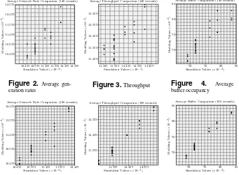
• Results comparison of scenario 1 where the simulation time is 120 seconds
Figure 2 shows that the simulation values of the aver-age data generation are not close to the modeling val-ues even they are incompact to distribute around the diagonaly = x. The difference is approximately in between from−4%to3%. Figure 3 shows that the simulation values are away from the modeling values, which the difference is approximately in between from
−4.8%to4.5%. The distribution of throughput values is incompact on the Figure 6. Figure 4 shows the av-erage buffer occupancies of sensor nodes also incom-pactly distribution on the figure. The difference of sim-ulation and modeling values is approximate between from−4%to4%. The result is not close to modeling values.
• Results comparison of scenario 1 where the simulation length is 180 seconds
Figure 5 shows that the simulation values are closer to the modelling values than the simulation in 120
seconds, which the difference is approximately in be-tween from −1%to1.5%. Figure 6 shows that the simulation values are closer to the modelling values than the simulation in 120 seconds, which the dif-ference is approximately in between from−1.2%to
1.2%. Figure 7 shows the difference of simulation and modeling values is approximate between from−1.6% to1.6%. The result is also closer than simulation in
120seconds. But it is hardly to present where the sen-sor nodes distribute on the figure.
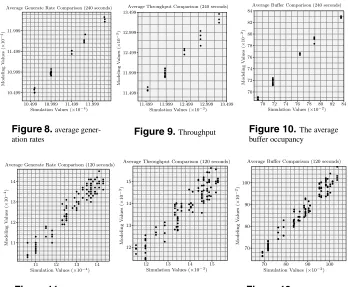
• Results comparison of scenario 1 where the simulation length is 240 seconds
Figure 8 shows that the simulation values are quite close to the modeling values, which the difference is approximate between from −1% to 1.5%. We no-tice that the results of running in 240 seconds is sim-ilar with running in 180 seconds Figure 9 shows that the simulation values are close to the modelling val-ues, which the difference is approximate between from
−1%to1%. Figure 10 shows that the simulation val-ues are close to the modelling valval-ues. We can see that the difference of simulation and modeling values is ap-proximate between from−1%to1.5%.
In summary, the simulating values in120seconds run-ning and the modeling values are not quite approach each other. Whereas in180and240seconds running, the simulating values are closer to modeling values than120seconds. This result validates that our sim-ulation need a long time running, almost 180or240 seconds, to match the model.
However, the result does not have persuasion for few nodes in a sensor network. So we increase the number of nodes in a sensor network to100nodes to compare the difference between two scenarios still in terms of three running time.
• Results comparison of scenario 2 where the simulation length is 120 seconds
Figure 11 shows that the simulation values are not very close to the modelling values, which the dif-ference is approximate between from −4% to 3%. The average generation rate of sensor nodes mainly concentrate on 0.000124to0.000144that means the average generation rate of most nodes are between
0.000124and0.000144. It also represents that the
10.499 10.999 11.499 11.999 12.499 12.999 10.499
10.999 11.499 11.999 12.499 12.999
Average Generate Rate Comparison (120 seconds)
Simulation Values (×10−4)
M
o
del
in
g
V
al
ues
(
×
10
−
[image:4.612.132.473.75.326.2]4)
Figure 2.Average gen-eration rates
11.499 11.999 12.499 12.999 13.499 11.499
11.999 12.499 12.999 13.499
Average Throughput Comparison (120 seconds)
Simulation Values (×10−3)
M
o
del
in
g
V
al
ues
(
×
10
−
3)
Figure 3.Throughput
70 75 80 85 70
75 80 85
Average Buffer Comparison (120 seconds)
Simulation Values (×10−2)
M
o
del
in
g
V
al
ues
(
×
10
−
2)
Figure 4. Average buffer occupancy
10.499 10.999 11.499 11.999 12.499 10.499
10.999 11.499 11.999 12.499
Average Generate Rate Comparison (180 seconds)
Simulation Values (×10−4)
M
o
del
in
g
V
al
ues
(
×
10
−
4)
Figure 5.average gener-ation rates
11.999 12.499 12.999 11.999
12.499 12.999
Average Throughput Comparison (180 seconds)
Simulation Values (×10−3)
M
o
del
in
g
V
al
ues
(
×
10
−
3)
Figure 6.Throughput
70 75 80 85
70 75 80 85
Average Buffer Comparison (180 seconds)
Simulation Values (×10−2)
M
o
del
in
g
V
al
ues
(
×
10
−
2)
Figure 7. The average buffer occupancy
This means that the buffer of each node stored the ference number of data units. We can see that the dif-ference of simulation and modeling values is approxi-mate between from−4%to4%. The result is also not close to modeling values.
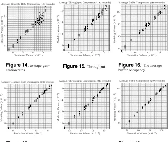
• Results comparison of scenario 2 where the simulation length is 180 seconds
Figure 14 shows that the simulation values are closer to the modelling values than the simulation in 120 seconds, which the difference is approximate between from −1.6% to 1.7%. The average generation rate of sensor nodes mainly concentrate on 0.000122 to
0.000142. It also represents that the sensor network
running in 120 seconds does not reach stable. Fig-ure 15 shows that the simulation values are closer to the modelling values than the simulation in 120 seconds, which the difference is approximate between from−1.6%to1.7%. The throughput of sensor nodes mainly concentrate on0.00132to0.00152. Figure 16 shows the average buffer occupancies of sensor nodes distribute uniformly on the figure. This means that the buffer of each node stored the difference number of data units. We can see that the difference of simula-tion and modeling values is approximate between from
−1.6%to1.7%. The result is also closer than simula-tion in120seconds.
• Results comparison of scenario 2 where the simulation
length is 240 seconds
The average generation rates of sensor nodes mainly concentrate on0.000122to0.00014. Figure 17 shows that the simulation values are quite close to the mod-elling values, which the difference is approximate be-tween from−1%to1.1%. The throughput of sensor nodes mainly concentrate on0.00132to0.0015. Fig-ure 18 shows that the simulation values are close to the modelling values, which the difference is approximate between from−1.1%to1.1%. Figure 19 shows the average buffer occupancies of sensor nodes distribute uniformly on the figure. This means that the buffer of each node stored the difference number of data units. We can see that the difference of simulation and mod-eling values is approximate between from−1.1%to
1.1%.
3.3
Comparison summary
In summary, the simulating values in100nodes scenario is much more accurate to present the nodes ’ behaviors than25nodes scenario in terms of average generation rate, throughput and buffer occupancy. The simulation is easy to modify the number of nodes in a sensor network to validate the result.
10.499 10.999 11.499 11.999 10.499
10.999 11.499 11.999
Average Generate Rate Comparison (240 seconds)
Simulation Values (×10−4)
M
o
del
in
g
V
al
ues
(×
10
−
4)
Figure 8.average gener-ation rates
11.499 11.999 12.499 12.999 13.499 11.499
11.999 12.499 12.999 13.499
Average Throughput Comparison (240 seconds)
Simulation Values (×10−3)
M
o
del
in
g
V
al
ues
(×
10
−
3)
Figure 9.Throughput
70 72 74 76 78 80 82 84 70
72 74 76 78 80 82 84
Average Buffer Comparison (240 seconds)
Simulation Values (×10−2)
M
o
del
in
g
V
al
ues
(
×
10
−
2)
Figure 10.The average buffer occupancy
11 12 13 14
11 12 13 14
Average Generate Rate Comparison (120 seconds)
Simulation Values (×10−4)
M
o
del
in
g
V
al
ues
(
×
10
−
4)
Figure 11.average gen-eration rates
12 13 14 15
12 13 14 15
Average Throughput Comparison (120 seconds)
Simulation Values (×10−3)
M
o
del
in
g
V
al
ues
(
×
10
−
3)
Figure 12.Throughput
70 80 90 100
70 80 90 100
Average Buffer Comparison (120 seconds)
Simulation Values (×10−2)
Mo
d
e
lin
g
V
a
lu
e
s
(
×
10
−
[image:5.612.130.478.73.360.2]2)
Figure 13.The average buffer occupancy
180seconds running the network reaches stable.
4
Conclusion
In this paper, we described in great details the approach of switching the sensor nodes between“sleep” and “activ-ity” states based on the Geometric distribution. We also demonstrated how to use the Markov chain to model the dynamics of sensor nodes. The DTMC based analysis is used to calculate the sensor node’s performance metrics in-cluding the throughput, the average generation rate and the average buffer occupancy. To validate the DTMC based an-alytic model, we run a large number of simulations for two scenarios.
The results showed that after a long time running, the simulation and modeling metrics are very close in terms of the average generation rate, throughput and average buffer occupancy. Moreover, through simulation we noticed that the sensor network become stable after 180 seconds run-ning.
In the future, we are going to extend the simulations and experiments to the general cases. We will investigate the performance of the sensor network, in which the changes of network architectures and topology may be studied further.
References
[1] Fan Ye, Haiyun Luo, Jerry Cheng, Songwu Lu, Lixia Zhang. A Two-Tier Data Dissemination Model for Large-scale Wireless Sensor Networks.MOBICOM02, September 2328, 2002, Atlanta, Georgia, USA.
[2] C.-F. Chiasserini and M. Garetto.Modeling the Perfor-mance of Wireless Sensor Networks. IEEE INFOCOM 2004.
[3] Qiangfeng Jiang, D. Manivannan.Routing Protocols for Sensor Networks.
[4] G. Asada, M. Dong, T. S. Lin, F. Newberg, G. Pot-tie, W. J. Kaiser.Wireless Integrated Network Sensors: Low Power Systems on a Chip.
[5] Wei Ye, John Heidemann, Deborah Estrin.An Energy-Efficient MAC Protocol for Wireless Sensor Networks. The Proceedings of the IEEE INFOCOM, 2002.
[6] Ian Downard, Naval Research
Labora-tory.SIMULATING SENSOR NETWORKS IN
NS-2.NRL Formal Report 5522-04-10, 2004.
11 12 13 14 11
12 13 14
Average Generate Rate Comparison (180 seconds)
Simulation Values (×10−4)
M
o
del
ing
V
al
u
es
(
×
10
−
4)
Figure 14.average gen-eration rates
12 13 14 15
12 13 14 15
Average Throughput Comparison (180 seconds)
Simulation Values (×10−3)
M
o
del
in
g
V
al
ues
(
×
10
−
3)
Figure 15.Throughput
70 80 90 100
70 80 90 100
Average Buffer Comparison (180 seconds)
Simulation Values (×10−2)
Mo
d
e
lin
g
V
a
lu
e
s
(
×
10
−
2)
Figure 16.The average buffer occupancy
11 12 13 14
11 12 13 14
Average Generate Rate Comparison (240 seconds)
Simulation Values (×10−4)
M
o
del
in
g
V
al
ues
(
×
10
−
4)
Figure 17.average gen-eration rates
12 13 14 15
12 13 14 15
Average Throughput Comparison (240 seconds)
Simulation Values (×10−3)
M
o
del
in
g
V
al
ues
(
×
10
−
3)
Figure 18.Throughput
70 80 90 100
70 80 90 100
Average Buffer Comparison (240 seconds)
Simulation Values (×10−2)
M
o
del
in
g
V
al
ues
(
×
10
−
[image:6.612.132.478.74.366.2]2)
Figure 19.The average buffer occupancy
MAC for Wireless Sensor Networks. In proceedings of the 1st International Workshop on Software for Sen-sor Networks (SenSen-sorWare) at COMSWARE06. New Delhi, India. January, 2006
[8] Bret Hull, Kyle Jamieson, Hari Balakrishnan. Miti-gating Congestion in Wireless Sensor Networks. Sen-Sys’04, November 3.5, 2004, Baltimore, Maryland, USA.
[9] Chieh-Yih Wan, Andrew T. Campbell, Lakshman Kr-ishnamurthy. PSFQ: A Reliable Transport Protocol for Wireless Sensor Networks.WSNA02, September 28, 2002, Atlanta, Georgia, USA.
[10] Rebecca Atherton, Leslie Hogben.A Look at Markov Chains and Their Use in Google. Iowa State Univer-sity, MSM Creative Component, Summer 2005.
[11] Hogben, Leslie. Elementary Linear Algebra. West Publishing Company, St. Paul, MN, 1987: 81-92
[12] Hefferon, Jim. (2003).Linear Algebra, chapter 3. Re-trieved 4/20/05 from
[13] National Council of Teachers of Mathematics (NCTM). New Topics for Secondary School Math-ematics: Matrices. Reson, VA: NCTM, 1988: 1, 2, 49-65, 96-98.
[14] Carter, Tamara; Tapia, Richard A.; Papakonstanti-nou, Anne. (1995-2003). Linear Algebra: An Introduction to Linear Algebra for Pre-Calculus Students, chapter 7, Retrieved 4/20/05 from http://ceee.rice.edu/Books/LA/index.html
[15] W. Rabiner Heinzelman, A. Chandrakasan, and H. Balakrishnan, Energy-Efficient Communication Pro-tocol for Wireless Microsensor Networks. 33rd Inter-national Conference on System Sciences (HICSS 00), Jan. 2000.
[16] A. Ephremides, Energy Concerns in Wireless Net-worksIEEE Wireless Communications, Aug. 2002.
[17] K. Fall and K. Varadhan.The NS Manual (Formerly NS Notes and Documentation. http://www.isi.edu/, 2002.
[18] Wei Ye and John Heidemann.Medium Access Control in Wireless Sensor Networks. USC/ISI TECHNICAL REPORT ISI-TR-580, OCTOBER 2003.