Geometric Properties and a Combinatorial Analysis of Convex Polygons Constructed of Tridrafters

RIT Scholar Works

Theses

5-10-2018

Geometric Properties and a Combinatorial

Analysis of Convex Polygons Constructed of

Tridrafters

Trevor Nelson

Follow this and additional works at:

https://scholarworks.rit.edu/theses

This Thesis is brought to you for free and open access by RIT Scholar Works. It has been accepted for inclusion in Theses by an authorized administrator of RIT Scholar Works. For more information, please contactritscholarworks@rit.edu.

Recommended Citation

Combinatorial Analysis of

Convex Polygons Constructed

of Tridrafters

by

T

revor

N

elson

A Thesis Submitted in Partial Fulfillment of the Requirements

for the Degree of Master of Science in Applied Mathematics

School of Mathematical Sciences, College of Science

Rochester Institute of Technology

Rochester, NY

Dr. Matthew Coppenbarger Date

School of Mathematical Sciences

Thesis Advisor

Dr. Darren Narayan Date

School of Mathematical Sciences

Committee Member

Dr. Hossein Shahmohamed Date

School of Mathematical Sciences

Committee Member

Dr. Matthew J. Hoffman Date

School of Mathematical Sciences

Abstract

The aim of this thesis is to show how the use of parity in tandem with the triangular grid as well as

a newly introduced and similar method are insufficient to provide proof for why convex regions composed

using the full set of shapes known as "proper tridrafters" have a portion shifted in a fashion known as

C

ontents

I Introduction 1

II Drafters 11

III Tridrafters 13

III.1 Construction of the Tridrafters . . . 13

III.2 Against-the-grain . . . 16

IV Analysis of the Fourteen Tridrafters 28 IV.1 A Parity Analysis of the Tridrafters . . . 28

IV.2 A Tri-Coloring Analysis of the Tridrafters . . . 38

IV.3 Combining Measurments . . . 41

V Measuring Solutions 48 V.1 Hexcombs of Solutions . . . 48

VI Conclusion 53 VII ACKNOWLEDGEMENTS 54 VIII Appendix 55 VIII.1 Closing Graphs . . . 55

VIII.2 Tridrafter Vectors In All Positions . . . 69

VIII.3 List of unique hexcombs . . . 81

VIII.4 Program Usage . . . 81

VIII.4.1Mathematica Program . . . 81

VIII.4.2 Cluster Network . . . 89

VIII.5 Hexcomb Measurements to Solutions . . . 90

L

ist of

F

igures

1 A solution to Haberdasher’s puzzle . . . 1

2 MacMahon square and triangle solution layouts . . . 2

3 Square and equilateral triangular lattice structures . . . 3

4 Bases from square lattice . . . 4

5 Bases from triangular lattice . . . 4

6 Polyominoes set examples . . . 5

7 4x5 Rectangle and Tetrominoes . . . 6

8 4x5 Rectangle and Tetrominoes Checkered . . . 6

9 Polyform Layouts (featuring pentominoes, hexiamonds, and heptiamonds) . . . 8

10 Eternity Region . . . 9

11 Sturdy and weak dodecadrafters . . . 9

12 First public solution . . . 10

13 Proper didrafters . . . 11

14 Improper didrafters . . . 12

15 The Fourteen Proper Tridrafters (Coloring within the figure has no significance) . . 13

16 Sample regions . . . 14

17 Trapezoid layout . . . 15

18 Tridrafters with and against-the-grain . . . 16

19 Four 30◦angles forming a 120◦angle . . . 19

20 The "T" Section . . . 22

21 Other convex tridrafter layouts . . . 23

22 The Aligned and Reflex Angles within Tridrafters . . . 25

23 ClosingT3 . . . 26

24 Up-down parity . . . 29

25 Left-Right parity . . . 29

26 East-west parity . . . 30

28 T1’s drafter orientations . . . 32

29 T_1’s Orientations Rotated and Reflected . . . 33

30 Coloring Orientations . . . 36

31 Parallelogram Region . . . 36

32 Two regions prepared for measurement . . . 37

33 Tri-coloring grid . . . 38

34 T1’s drafter positions on tri-coloring grid . . . 39

35 Hexcomb measuring table . . . 50

36 Coloring for hexcomb values . . . 50

37 ClosingT1 . . . 55

38 ClosingT2 . . . 56

39 ClosingT3 . . . 57

40 ClosingT4 . . . 58

41 ClosingT5 . . . 59

42 ClosingT6 . . . 60

43 ClosingT7 . . . 61

44 ClosingT8 . . . 62

45 ClosingT9 . . . 63

46 ClosingT10 . . . 64

47 ClosingT11 . . . 65

48 ClosingT12 . . . 66

49 ClosingT13 . . . 67

50 ClosingT14 . . . 68

L

ist of

T

ables

2 Color values by position . . . 41

4 Two actions . . . 44

5 Two action parity . . . 45

6 Two actions tri-coloring . . . 46

7 Identity hexcombs . . . 69

8 σhexcombs . . . 70

9 σ2hexcombs . . . 71

10 σ3hexcombs . . . 72

11 σ4hexcombs . . . 73

12 σ5hexcombs . . . 74

13 τhexcombs . . . 75

14 στhexcombs . . . 76

15 σ2τhexcombs . . . 77

16 σ3τhexcombs . . . 78

17 σ4τhexcombs . . . 79

I.

I

ntroduction

Since times ancient we as humans have set ourselves apart from other animals by having a curiosity

on how things work; even if the mechanism isn’t relevant to other branches of science at the time.

How might seemingly different things be put together to create a larger whole? We’ve entertained

ourselves with such a concept; often in the form of puzzles. Puzzles allow us to acquire knowledge

on how the small individual parts we’re given work together to create something larger than the

some of those parts. Geometric puzzles, logic puzzles, or even word puzzles can allow us to see

how we may approach problems in various fashions as there may be multiple solutions to the same

riddle. We see how things that look different can interlock with one another and be similar despite

the apparent first impression they may give. With this curiosity, we now have a tremendous

amount of geometric puzzles that have been created throughout human existence.

Some puzzles start with a whole and have us create the parts. Haberdasher’s puzzle is one

of the best known solved puzzles of this kind. We are asked "Can one take an equilateral triangle

and dissect it such that the pieces created can be reconfigured into a square?" Henry Dudeney

first proposed this question in 1902. After discussion with other mathematicians, an interesting

solution was found. Not only can the triangle be dissected, but the triangle may be separated into

four "hinged" pieces such that they could be swiveled to create the square solution as shown in

Figure 1 [16]. From this alone one may list an infinite number of solutions.

Figure 1:A solution to Haberdasher’s puzzle

Geometric puzzles will often make use of polygons for the creation of their individual

pieces or a specific polygon as the ending form of the overall goal.

Definition 1. Apolygonis a bounded region upon a flat plane whose boundary consists of a finite number of line segments, each of finite length, and each line segment intersects with exactly two

segments areverticesof the polygon. (E.g. the square has four sides and four vertices; the triangle has three sides and three vertices.)

Jigsaw puzzles will usually form a rectangle when joined together to create the intended

solution. Other puzzles make use of the grouping of similar polygons such as McMohan squares

and triangles. This puzzle utilize tiles with a color along each edge and each pair of tiles joined

alongside edges must match in color. These types of puzzles most often work with congruent

polygons which are also often regular such as squares, equilateral triangles, or some other relatively

simple shape. We are not limited to this though; see Fredrickson [3] for a comprehensive overview

of dissection puzzles.

Figure 2:MacMahon square and triangle solution layouts

What of creating other geometrical figures? Tessellations are things that have captivated

the attention of people both inside and outside of the mathematical community. Some of these

creations are simple enough to observe for anyone to be intrigued upon examining such work.

A very famous figure, perhaps the best known, would be M.C. Escher who has drawn the

attention of the entire world through his use of the mechanics of isometric relationships. We

create cells, one comprised of squares and the other of equilateral triangles, that might act as such

a foundation.

Figure 3:Square and equilateral triangular lattice structures

Alattice Lcan be regarded as a regular tiling of the plane by a primitive cells forming a set of edges. For our purposes, we will only utilize squares and equilateral triangles as our primitive

cells. (One more case will be utilized later)

With any particular lattice, we may utilize part of (Figures 4(a) and 5(a)), the whole of

(Figures 4(b) and 5(b)), the union of cells (Figure 5(c)), or the union of parts of cells (Figure 4(c))

to create abase; an alpha to start with when creating polygons of greater complexity. There are arguably an infinite number of bases that may be created. Schattschneider’s work [13] provides a

we will restrict our usage of lattice structures to squares and equilateral triangles.

Figure 4:Bases from square lattice

Figure 5:Bases from triangular lattice

Any puzzle involving physical pieces, for many, are the simplest to understand or at least

attempt due to their "hands on" nature. We take a set of figures created under a set of rules and

create a larger whole often using each element within the set constructed. Tiling puzzles are

perhaps the most versatile of these; they have complexities that range from the very simple to the

extreme. Solomon Golumb tackled many different puzzles dealing with polyominoes, which he

created in 1955 [4], shapes similar to dominoes but are not restricted to the rectangle formed by

two halves that are well known. Figures will later be introduced which are constructed in a similar

manner. To understand how the polyominoes are constructed we must be familiar with a few terms.

create two congruent polygons; distinct chirality does not make two polygons non-equivalent.

Definition 4. Theorderof a polyomino is determined by the number of bases utilized to form it. Definition 5. Two polygons areisometriesof one another if one may undergo a series of distance-preserving transformation between metric spaces.

Figure 6:Polyominoes set examples

One may question "How we know the sets given in Figure 6 are complete?" For example,

why aren’t there more of order 2? One could rotate the red polyomino shown to create a horizontal

version of this, but it is still far too similar to the original. The best known polyominoes are

perhaps the tetrominoes [4] which are seen in the game of Tetris which utilizes polyominoes of

order 4. One may argue that more polygons should be present in this set but these would be

isometries or equivalencies of polyominoes that already exist within the list shown.

What sort of puzzles can be created with these tetrominoes? These five elements have a

total area of 20 square units as each is made up of four squares. A natural question to ask is if it

possible to form a 4×5 rectangle using these five tetrominoes as pieces? We can prove that this is

impossible.

Take the 4×5 rectangle and checker the unit squares black and white so that each unit

square is of an alternate color to those orthogonally adjacent. Do the same with the five different

tetrominoes.

We see that four of the five pieces are balanced; each has the same number of black and white squares. The "T" however is imbalanced as it will have one white and three black or vice

Figure 7:4x5 Rectangle and Tetrominoes

Figure 8:4x5 Rectangle and Tetrominoes Checkered

white squares and 10 black squares. Due to the imbalance of our five pieces we will have either 8

white squares and 12 black squares, or 12 and 8 respectively. It is therefore impossible to lay the

five pieces upon the 4×5 rectangle. This is often referred to asparity-imbalance.

An interesting observation comes up when we construct the next set of polyominoes, each

new set an order larger than the last by 1. Looking at the number of unique polygons that may

be constructed: when composed of a single base square there is 1 figure, with two squares again

1 figure, with three there are 2, then 5, 12, 35, 108, 369, and the list keeps growing. There is no

specific formula for determining the quantity of polyominoes there will be of a specific order, but

we are able to place bounds on the cardinality of a set of polyominoes of a given order utilizing

Klarner’s Constant, the limit growth rate of polyominoesλfor polyominoes of ordern.

This value is discreetly discussed in the Barequet’s paper [1]. Their paper also provides

proof for providing an upper bound for the growth rateλ ≤4.5685, which is at this point the

most accurate upper bound forλ. The lower bound until recently was 3.98, but has recently been

With this knowledge in hand, it would give credit to the idea that the cardinality of sets

utilizing any particular base, varying in order, will increase in a similar manner with some form

of growth rate constant. Likely not the same, but the notion tells us that the set of any ordernwill always be finite in number.

Different sets of pieces have been created with the same method to that of polyominoes, but

with a different base [10].

Definition 6. Apolyformis an element of a set of polygons constructed by using a polygon as a base and joining copies under a set of given rules.

Definition 7. Aregionis a polygon with an area correlating to a specific set of polyforms. Polyforms simpler to understand and recognize utilize regular polygons as their base

(Figures 4(b) and 5(b)). Figure 9 shows examples of polyforms, varying in base and order, in

recognizable configurations. Both a simple and more complex layout is provided [5]. The first pair

utilizes pentominoes; a set of polyominoes of order 5. The second pair utilizes hexiamonds; a set

of polyforms made using a lattice such as shown in figure 3(b) and creating a set of order 6. The

last uses heptiamonds; similar to hexiamonds but of order 7. A comprehensive list of polyiamonds

is made available through Goodger’s work [5].

We take special note of these regions as they form a recognizable shape or pattern overall,

but these examples are a drop within the plethora of regions that could be constructed using the

three polyform sets mentioned.

LetPbe a set of polyforms (such as the set of pentominoes or a subset of hexiamonds). Let

Rbe a region on the plane. LetAbe a function that takes in eitherPorRand give a real number to represent the area of all polyforms in the setPor the area enclosed within the regionR. These areA(P)andA(R)respectively. WhenA(P) =A(R), we look to see if we may exhaustPand lay each polyform within the regionRsuch that there is no space left withinRleft uncovered. Such a layout(s), if it exists, is called asolution.

Triangles have the least number of sides and vertices possible for a polygon, it’s impossible

Figure 9:Polyform Layouts (featuring pentominoes, hexiamonds, and heptiamonds)

it may be compiled by some finite quantity of triangles. O’ Rourke’s work [9] utilizes computers

to prove and expand upon this. Once done creating polyform sets using regular triangles (like the

hexiamonds and heptiamonds), it’s natural to consider a set based on a slightly more complex

form; which brings us to the base shape for creating the set of polyforms this paper focuses on:

thedrafterwhich is a 30◦-60◦-90◦triangle scaled to have an area of 1 unit.

In 1999, a Scottish enterprenour Christopher Monckton created a set of pieces using the

drafter as a base. He offered a prize of one million pounds to anyone who could offer a solution to

his challenge, the Eternity Puzzle, within four years of the puzzle’s release. A regular dodecagon,

shown in Figure 10 [2] was given for any to attempt to find a solution using provided pieces, a

sub-set of dodecadrafters, which is the set of polyforms of order 12 that utilize the drafter as a

base.

Only 209 of the set of 52630 possible dodecadrafters, no two being equivalent, were provided.

Any dodecadrafters that that formed holes were excluded. Also, the pieces had no 30◦ vertices or "weakly hanging" triangles that could be easily broken apart upon handling. This was to ensure a

"safer, sturdier" puzzle. A sturdy and weak example are shown in Figure 11 on the left and right

Figure 10: Eternity Region

were provided have specific (or lack of) properties.

Figure 11:Sturdy and weak dodecadrafters

Half of prize money was put up by Christopher Monckton himself. The other half was

provided by underwriters within London’s insurance market. All solutions were to be mailed

in and looked over on September 21 of 2000. If no solution was deemed correct, the following

mailed in solutions would be looked over on September 30, 2001. This was to repeat until the year

of 2003.

find a solution. He calculated that there were 10500possible attempts at creating solutions. Given

the puzzle’s size, Monckton believed the puzzle "intractable" [14]

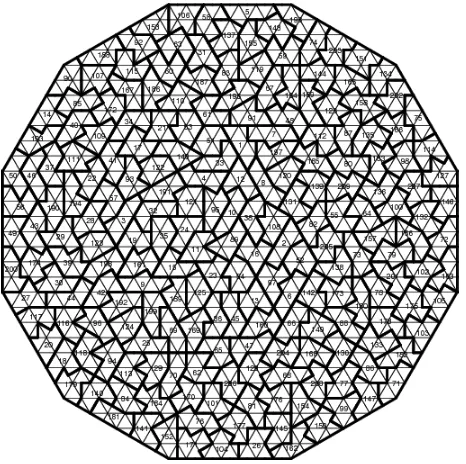
Figure 12:First public solution

The prize was claimed by Alex Selby and Oliver Riordan’s a year later; their solution is

shown in Figure 12. This solution was simply the first to be mailed in and accepted according to

the rules given for said challenge. After the challenge had been completed, Cristopher Monckton

apparently had to sell his home in order to pay this prize. Years later he made a statment that

said his claim was a PR stunt meant to boost sales. Another solution was subsequently found

by Guenter Stertenbrink [6], and there are many others. These solutions do not match clues that

were given with the puzzle from Monckton describing his solution layout and Monckton never

published his solution; this would imply that there are countless other solutions waiting to be

II.

D

rafters

Here, we introduce a simpler version of what was utilized in the eternity puzzle: polyforms of

order 2 that use the drafter as a base.

Definition 8. A polydrafteris a polyform with a drafter used as a base and is constructed by joining drafters such that each is joined with at least one other by edges of non-zero length.

Definition 9. Given any polyformP, when possible to be placed such that each individual base rests entirely within a cell of the grid the base was made from, the polyform isproper. Otherwise, it isimproper.

We will be focusing on the didrafters which are proper of which there are six. They are

constructed and labeled asD1throughD6in Figure 13.

It’s important to note that under the conditions laid out for creating polydrafters, they aren’t

necessarily proper. Examples of improper didrafters are shown in Figure 14. The quantity of

improper didrafters is infinite. One could take any proper didrafters and translate one of the two

drafters alongside the edge shared between the two any length.

III.

T

ridrafters

III.1

Construction of the Tridrafters

From the didrafters (Figure 13) we constructtridraftersby adding a third drafter to any of the didrafters such that the new polyform is proper. This results in a polydrafter of order 3. An

analysis of the tridrafters will be the main focus for the remainder of this thesis.

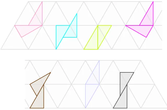
Figure 15 shows the complete set of tridrafters that may be constructed with this process.

For example,T1throughT4may each be constructed by adding a drafter toD6.

Let us scale the lattice such that the area of the cells is 2; this makes the area of a single

drafter 1. Using 14 tridrafters, each having an area of 3, any polygon constructed by joining them

together will have an area of 42. Any regionRwith an area of 42 may have a solution.

In Figure 16 below, there are regions with an area of 42 which may or may not have solutions.

For simplicity, the regions chosen are convex and symmetrical.

Figure 16: Sample regions

Though a region may have an area of 42 drafter units, this does not imply that a solution

exists for it. The elongated trapezoid in Figure 16 for example. Bernd Karl Rennhak of Germany

has made use of his own program and verified with the "Logelium Solver" that there are a total

of 1516 possible convex regions with the needed area that can be considered. Additionally, only

These numbers have been verified by other programs used to find solutions to puzzles in general,

resulting in exhaustively finding all regions with every unique solution. The other trapezoid

region, Figure 17, has two solutions and are simpler to observe than others as its edges conform

to the edge set of the triangular lattice and will be the main reference for explaining properties

found in all solutions.

III.2

Against-the-grain

The tridrafters that are utilized to form solutions for regions, defined as being proper, have the

capability of being placedwith-the-grain; a state of being placed in alignment with the lattice grid. While this is true for all the tridrafters individually, when two Tridrafters are connected they

are not necessarily placed with-the-grain simultaneously. Figure 18 shows two tridrafters placed

with-the-grain on the left and the same two tridrafters placed against-the-grain to the right.

In the figure below, we see the triangular lattice constructed utilizing the black nodes.

Lines can be drawn through these black nodes to form the triangular lattice used to created

the tridrafters. Each of the red nodes represents a midpoint between each pair of black nodes.

When tridrafters are placed with-the-grain together such as the pair on the left, the vertices of the

hypotenuse lie upon the black nodes forming an equilateral triangle between the drafters joining

the tridrafters.

We describe placement asagainst-the-grianwhen this does not occur. When a tridrafter is placed against-the-grain but the vertices that make up the hypotenuse lies upon red midpoint

nodes instead, it is placedorthogonally against-the-grain. Note how here a parallelogram is formed between the drafters joining the tridrafters.

Figure 18:Tridrafters with and against-the-grain

A solution for a region is with-the-grain if and only if all tridrafters within the solution lie

with-the-grain simultaneously. A solution for a region is against-the-grain otherwise.

region’s border. In trying to do so we often come to a point where we are seemingly forced to

cross the border or create a hole which is impossible to fill. This is known as abreachand avoid

respectively.

The trapezoid has four corners, two of which measure 60◦ and the other two 120◦. These will act as our starting locations for the placement of tridrafters to look into how our potential

solutions would need to be structured. The first corners to look at will be the 60◦corners. We may use a single tridrafter that contains a 60◦ angle or two tridrafters that contain 30◦angles to fill in a corner of this measurement.

Lemma 1. Either both T1and T7are placed in the60◦corners of the trapezoid, or one of the two are used

with the other corner being filled with T2, T5, or T6; two of these three used in tandem with one another.

Proof. There are two different methods to fill a 60◦corner. Utilize a single tridrafter that contains a 60◦angle or by connecting two 30◦corners of two individual tridrafters.

OnlyT1andT7contain a 60◦angle and can be placed in said corner with-the-grain. Of the tridrafters that contain 30◦corners, onlyT2,T5, andT6(only one of its three angles) can be used without causing a breach or a forming a void.

The 120◦corners are larger and therefore have a wider spread of choices for how to fill them. We may use a single tridrafter that contains a 120◦angle, use two tridrafters that contain a 90◦ angle and 30◦angle between them, use two tridrafters that contain two 60◦angles between them, use three tridrafters that contain a 60◦and two 30◦angles between them, or use four tridrafters that contain four 30◦angles between them.

Corollary 1.1. It is impossible to fill a120◦corner utilizing only tridrafters with60◦angles as only T1

and T7have the necessary60◦angles to be joined to fill in said corner and at least one must be placed to fill

a60◦corner.

Lemma 2. Only T1or T7exclusively may be used to fill in a120◦corner.

Lemma 3. To fill in corner larger than60◦ utilzing a90◦angle, the90◦angle must be formed by two individual drafters.

Proof. The 90◦ angles may be formed by either individual drafters or two joined drafters. The former with the altitude and base of the drafter acting as edges of the overall tridrafter. The

latter with the 60◦and 30◦angle being joined. Should the single drafter be used, it will always lie against-the-grain. Thus we are forced to utilize tridrafters with 90◦ angles formed by two individual drafters.

Lemma 4. It is impossible to have a with-the-grain solution utilizing two tridrafters connecting a90◦and

30◦degree angles to fill in the120◦corner of the trapezoidal region.

Proof. From Lemma 3, onlyT1,T2, andT8may be utilized for their 90◦angles.

WhenT1is placed in one of the 120◦such that its 90◦angle is covering part of the corner, of the remaining tridrafters to connect to it to fill this corner: IfT2is utilized, onlyT7orT8may be attachedT2’s right angle. Using the former would violate Lemma 1. When using the latter, only

T5andT6can be attached toT8. In connecting tridrafters toT8, choices that don’t cause breaches or voids will cause a hole in the shape ofT1to form. As this is already being utilized, we cannot fill said hole. IfT5is utilized, due to Lemma 1,T2andT6along withT7 are placed in the 60◦ corners. At this point, no tridrafters can be joined toT5without causing breaches or voids. If

T6 is utilized, due to Lemma 1,T2andT5 along withT7 are placed in the 60◦ corners. At this point, no tridrafters can be joined toT5without causing breaches or voids. IfT7is utilized, we breach Lemma 1. IfT8is utilized, a 120◦angle is formed; it will not be possible to fill this. IfT9is utilized, onlyT7orT8can connect to it. When usingT7, we breach Lemma 1. When usingT8,T2 andT6can connect to it. When usingT2,T5andT6must be used with one another to connect to

without causing a breach or a void.

WhenT2is placed in one of the 120◦corners such that its 90◦angle is covering part of the corner, of the remaining tridrafters to connect to it to fill this corner: OnlyT5may be connected to fill this corner. Nothing can connect toT5without causing breaches or voids.

WhenT8is placed in one of the 120◦such that its 90◦angle is covering part of the corner, of the remaining tridrafters to connect to it to fill this corner: IfT2is utilized, onlyT7can connect to it. At this point,T5,T6, andT1must be placed in the 60◦corners. IfT5andT6are placed in the 60◦ on the same side asT8,T1must be placed on the other. Nothing can connect toT1. IfT1is placed in the 60◦on the same side asT8,T5andT6must be placed on the other.T5andT6may be oriented in two different ways; either will result in nothing but breaches or voids when other

tridrafters are joined to them.

It is therefore impossible to have a with-the-grain solution utilizing two tridrafters to form

a 120◦angle using a 90◦and 30◦ angle between them.

Lemma 5. It is impossible to fill a120◦corner using four30◦ angles from four tridrafters and have a with-the-grain solution.

Proof. There are very few unions of Tridrafters that create 120◦angles from four 30◦angles. One is shown in Figure 19; these four tridrafters (T2,T5,T6, andT8) only work due to their elongated nature allowing for us to maneuver the pieces around.

Figure 19: Four 30◦ angles forming a 120◦angle

unavailable, we cannot fill in a 120◦corner in this way.

Lemma 6. It is impossible to utilize both T1and T7to cover both60◦ corners of the region and have a

with-the-grain solution.

Proof. Assume that bothT1andT7are utilized for their 60◦angles to fill the two 60◦corners. This will leave the 120◦angles to be filled by other means. From Corollary 1.1, Lemma 4, and Lemma 5, we may conclude that only utilizing three tridrafters, one with a 60◦angle and the other two with 30◦ angles are available. OnlyT5,T13, andT14 have 60◦ angles and are available. WhenT5is placed so that its 60◦angle is placed within the 120◦ corner such that it lays with-the-grain, it may be oriented in one of two ways. In either, onlyT2,T6, orT8may connect to it specifically alongside

T5’s longest edge. IfT2is utilized, onlyT8may join to it. Doing this causes a 120◦corner to form; there are no combinations of tridrafters available to fill in this newly formed corner. WhenT13 is placed so that its 60◦angle is placed within the 120◦ corner such that it lays with-the-grain, a void is formed. WhenT14 is placed so that its 60◦angle is placed within the 120◦corner such that it lays with-the-grain, a void is formed.

It is therefore impossible to utilize bothT1andT7for both 60◦corners of the region. This allows us to replace Lemma 1 with the following as follows:

Lemma 7. Either T1or T7exclusively is placed in the60◦corner of the trapezoid with the other corner

being filled with T2, T5, or T6; two of these three used in tandem with one another.

Lemma 8. Either T1or T7’s120◦corners must be utilized to fill one of the120◦corners of the region to

create a with-the-grain solution.

Proof. From Lemma 4, Lemma 5, and Corollary 1.1 we can conclude that the only ways to fill the 120◦corners is withT1orT7’s 120◦angle and a combination of one 60◦angle with two 30◦angles, or two combinations of the latter.

corners such that it’s 60◦angle covers part of the 120◦corner and lays with-the-grain, the other is immediately reserved for one of the 60◦corners by Lemma 7 andT5must be placed in the other 120◦corner. WhenT5is placed in one of the 120◦corners such that it’s 60◦angle covers part of the 120◦corner and lays with-the-grain, it may be placed in one of two orientations. With both, onlyT2,T6, andT8may connect to it alongside its longest edge. IfT2is utilized we violate Lemma 7. IfT6is utilized we violate Lemma 7. IfT8is utilized we cause a void. ThereforeT5cannot be utilized to fill in a 120◦corner. Thus there are not enough eligible 60◦angles to be used with this method to cover both 120◦corners.

Corollary 8.1. It is impossible to create a with-the-grain solution utilizing a60◦angle with two30◦angles between three tridrafters filling a120◦corner.

Through the use of these lemmas, we are able to conclude the following theorem.

Theorem 9. It is impossible to have a with-the-grain solution for the trapezoidal region.

Proof. By Lemma 4, it’s impossible to fill either 120◦corner by using two tridrafters, one with a 30◦angle and the other with a 90◦angle. By Lemma 5, it’s impossible to fill a 120◦corner using four tridrafters with 30◦angles. By Corollary 8.1, it’s impossible to fill a 120◦corner using a 60◦ angle with two 30◦ angles between three tridrafters. We may then use onlyT1andT7to fill in either 120◦corner. In doing so, by Lemma 7, the use of one will remove the possibility of using the other for the second corner. At this point, we have no valid options to fill in the second 120◦ corner.

As there is no with-the-grain solution for the trapezoid due to the interaction between the

tridrafters often being forced to cause breaches or voids, a natural query would be if it’s just as

difficult to create a with-the-grain solution for any convex region.

Conjecture 1. Every solution to a convex region will have tridrafters placed against-the-grain.

This is what we wish to prove due to the lack of any counter-proof to this claim from any

discovered solutions to any region.

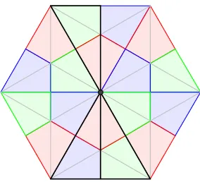
Figure 20 shows a solution for the trapezoidal region in tandem with a drafter grid that

trapezoid region is composed of 21 full cells or 42 drafter units. At first glance, the tridrafters as

placed in the given solution, may appear to be with-the-grain. Looking closer though, one can

observe that there is a section of four tridrafters that exhibit the against-the-grain trait. These 4

pieces are with-the-grain in relation to one another as shown in Figure 20 in gold. The other 10

tridrafters are with-the-grain in relation with one another as well shown in green. This solution

has two different underlaying drafter grids, the one in gold and the one in green.

Figure 20: The "T" Section

There is only one other known solution to the trapezoid region crafted by removing the

four tridrafters in the gold area that make up the "T" section out, performing an action of vertical

reflection on all four tridrafters, and placing them back in the same "T" section which will have no

effect upon the gold and green drafter grids drawn in Figure 20. Looking at these two colored

drafter grids we see that the smaller gold portion is similar to the green drafter grid. It’s as if the

original grid shifted horizontally so that what would be black nodes in Figure 18 were now at red

nodes. It seems that if we’re to find a solution we’ll have a sub-region that does not rest upon the

A solution for two different convex shapes are shown displaying this same feature in

Figure 21. The green and yellow grids that lay beneath the solutions illustrate the against-the-grain

grid shift between the two sub-regions. The right configuration shows that regions with the same

underlying grid can be entirely disjointed from one another similar to the trapezoid region’s

solutions.

Figure 21:Other convex tridrafter layouts

This characteristic is identified most easily with what was shown in Figure 18 Tridrafters

are placed orthogonally against-the-grain and form parallelograms similar to the third improper

didrafter depicted in Figure 14 rather than equilateral triangles when joined.

Another natural question that may arise is "Why is this characteristic so common?" There

are facts about this set of 14 tridrafters that give credence to the idea of the against-the-grain

property of being common, if not necessary. Let’s first assume that a person is attempting to create

solution that is with-the-grain.

Definition 10. A polydrafter hasacute valenceif it has at least one concave angle present.

The degree of acute valence will vary depending on how many concave angles are present.

T1/2/5 have an openness of degree 0,T3/4/6/7/8/13/14of 1, andT9/10/11/12 of 2.

LetPbe a polygon constructed of joined tridrafters that is concave due to an arbitrary angle

linked toPsuch that the resulting polygon is convex, we say that T hascompletedθ.

Definition 11. A polygon hasconvex completionif there is no internal angleθwhich has a value

greater than 180 degrees.

Theorem 10. To create a convex polygon when linking Tridrafters, altitudes must be linked to close it. Proof. Assume two tridraftersTmandTn are linked together. Assume one of the tridrafters,Tnhas an open 270◦ angle. The 270◦degree angle must be closed for the resultant polygon to be convex. This can only be done by linking tridrafterTmwith a 90◦corner to the 270◦corner of tridrafterTn. 90◦ angles are present only with the right angle of a single drafter, formed by the altitude and base acting as the rays of the angle, or the joining of a 60◦and 30◦ angle between two drafters, formed by the altitude and hypotenuse acting as the rays of the angle of said two drafters. If we

utilize the former to close, either the base or altitude ofTmmust link to the altitude ofTn. If the base is used to link the two, the result will not be convex. If the altitudes are linked, the result

may be convex. If we utilize the latter to close, either the hypotenuse or altitude ofTmmust link to the altitude ofTn. If the hypotenuse is used to link the two, the result will not be convex. If the altitudes are linked, the result may be convex. Thus, tridrafters must be linked by altitudes to

create a resultant convex polygon.

Theorem 11. To create a convex polygon with-the-grain, the270◦angle must be closed utilizing a right angle formed by a single drafter. (This will be referred to as an aligned angle).

Proof. Assume tridrafter Tn is open. Assume two tridraftersTmis closingTn. Assume the two tridraftersTmandTn lie with-the-grain in relation to one another. Based on the first theorem we must use the altitude from a right angle formed from a single drafter or the right angle formed by

two drafters. If we link altitudes of right angles formed in the latter format, an against-the-grain

Figure 22 depicts all tridrafters and labels the reflex and aligned angles.

Figure 22:The Aligned and Reflex Angles within Tridrafters

Theorem 12. All aligned angles must close a270◦open angle.

Proof. Assume all tridrafters are aligned with-the-grain Assume the tridrafters all fit within a convex region with an area of 21 cells There are a total of fifteen 270 degree internal angles

between the 14 tridrafters. There are a total of fifteen aligned angles. Each of the fifteen 270 degree

internal angles must be closed to prevent the resultant polygon from being concave. Thus, to

create a convex with-the-grain configuration, there must a 1:1 utilization between each 270◦and 90◦angle.

Looking at these theorems, it’s would seem prudent to observe what type of layout emerges

when we close one tridrafter with a second. The goal is to create a fully closed polygon so we’ll

take a look into if, when closed, the degree of openness is reduced, remains constant, or increases.

In the graph below, Figure 23, shows what occurs when each tridrafter is used to close tridrafter

Figure 23:ClosingT3

The shape of each node shows how many available right angles the tridrafter has, or how

many options there are to close an open tridrafter. Circles have zero available right angles, triangles

have one, and squares have two. The coloring of said nodes represents the degree of openness of

the tridrafter. Uncolored nodes have a degree of 0, blue nodes of 1, and black nodes of 2. Lastly,

the color of the arcs joining the 13 tails to the featured head, the tridrafter in the center, represents

how the degree of openness changes upon closing. Green represents that no new concave angles

are formed causing the degree of openness to fall by 1, yellow represents that one concave angle

is formed keeping the degree constant, orange represents that two concave angles are formed

increasing the degree by 1, and red represents that three concave angles are formed causing the

degree to increase by 2.

All graphs of this nature can be found in VIII.1 in the appendix section.

Due to the nature of the tridrafter, verified by the graphs shown, we can observe a few

tail end of an arc as they have no available right angles to close an open angle. Triangular nodes

will act as a tail for one arc per right angle present in the tridrafter being closed. Square nodes will

act as a tail for two arcs per right angle present in the tridrafter being closed. Uncolored nodes

will never be on the head end of an arc as they have no open angles that need to be filled.

Looking at each of these 14 graphs, we see that onlyT1andT2have the capability of closing another tridrafter and reduce the degree of openness. This at least lends a strong argument for

the idea that when attaching tridrafters together with-the-grain, a concave shape will result as all

IV.

A

nalysis of the

F

ourteen

T

ridrafters

IV.1

A Parity Analysis of the Tridrafters

According to the results of Rennhak’s program, and assuming it’s complete [12], we know of every

solution to every possible convex region. We know then that it’s impossible to create a convex

solution with every tridrafter to be with-the-grain simultaneously. Hence our conjecture is true,

but there is no underlaying mathematical reason to explain this. How does one go about trying to

prove why a with-the-grain convex solution is impossible? The first thing done here is creating a

method to mathematically quantify the pieces of the puzzle. We do this in two different ways.

The first method uses the idea parity mentioned earlier. We create parity patterns by shading cells

upon planes which are created in similar matter to those found and described in Levine’s paper [7]

on Plane Symmetry Groups. We’re ensured the plane will repeat itself infinitely as it’s generated

in a manner conforming to the ideas established from Schattschneider’s work [13].

Take an equilateral triangle on the plane with edge lengths of 2. Make one edge rest upon

the x-axis and one vertex the origin point. Suppose all points of the triangle are rotated by π

3/60◦ about either endpoint to form a new triangle. Repeat this six times to form a hexagonal cluster of

six cells. Color the upwards oriented cells black and the downwards oriented cells white. Suppose

that every point on the plane is translated to the right by 6 withT1(~x) =~x+ (6, 0)and translated diagonally up and right byT2(~x) =~x+ (3,

√

3). Repeating this action creates an infinite plane

Figure 24:Up-down parity

Take the same triangular lattice to form the same hexagonal cluster of cells. Draw six

altitudes, one for each triangle, starting from the vertex that is the center of the hexagonal cluster.

This will create 12 half cells, drafters, and we will color the drafters black and white alternatively.

Suppose that every point on the plane is translated to the right by 6 withT1(~x) =~x+ (6, 0)and translated diagonally up and right byT2(~x) =~x+ (3,

√

3). Repeating this action creates an infinite

plane with a pattern that will be referred to as theLeft-Rightparity, Figure 25, with relative size for our use.

Figure 25:Left-Right parity

Take the same triangular lattice to form the same hexagonal cluster of cells. Draw six

altitudes, one for each triangle, starting from the vertex that is the center of the hexagonal cluster.

This will create 12 half cells. Within one of these six cells we will color 1 of the halves black and

then the second black. We will continue this pattern for all six cells. Suppose that every point on

the plane is translated to the right by 6 withT1(~x) =~x+ (6, 0)and translated diagonally up and right byT2(~x) =~x+ (3,

√

3). Repeating this action creates an infinite plane with a pattern that

will be referred to as theEast-Westparity, Figure 26, with relative size for our use.

Figure 26:East-west parity

The following figure, Figure 27, divides the hexagonal area into 12 half-cells. Giving value

to these half-cells, 1 to the shaded and−1 to the unshaded, allows us to assign value that can

describe the tridrafters relative to the various orientations they may be placed in.

Figure 27: Numbering of the different orientations of the half-cell

We follow this process to give a value to the polydrafter.

2. Separate the polydrafter into thennumber of drafters that compose it while maintaining the individual drafter’s orientation.

3. Place each drafter upon the single one of the twelve orientations the piece will fit into.

4. Give the value of 1 to the drafter if placed in a shaded half-cell or a value of -1 if placed into

an unshaded half-cell.

5. Add thennumber of values together; this sum will be referred to asa.

6. Repeat process with the left-right parity to obtainb; repeat process with the east-west parity to obtainc.

We use these three parities which were created by Ed Pegg Jr. [11], not necessarily created

from the above explanations, they are just processes of recreating said patterns.

If we apply these patterns to our lattice and place our drafters upon the grid, then we are

able to give three values to each drafter and therefore tri-drafter, one from each parity. When

we place a drafter onto the grid for one method, it stays in that same orientation for the other

methods; only the grid pattern behind it is changed to give the other needed values.

It is important to keep in mind that we arenotplacing the entire tridrafter into the grid as one piece. We are looking at the orientation of each individual drafter that composes the

polydrafter, measuring each of their values, and then adding all values together. An example

with T1is given in Figure 28. We see a drafter with an orientation of 2, 7, and 8. These three drafters have parity measurements ofh−1,−1, 1i,h1, 1, 1i, andh1,−1,−1irespectively. Adding

Figure 28:T1’s drafter orientations

Definition 12. LetRbe a figure (polydrafter, region, etc.). We definepas the function that takesR

and maps it to the 3-dimensional vectorha,b,ciwherea,b, andcare the parity values as defined in the measuring process. We callha,b,citheparity vectorofR.

As a tridrafter can be placed into the grid in a multitude of ways there are multiple parity

vectors associated with each tridrafter. This vector will alter whenever the tridrafter is rotated

60◦represented by the actionσ, or reflected represented by the actionτ. Ultimately, any single

tridrafter may have one of four parity vectors, very similar in composition, dependent on its

Figure 29 shows the effects of rotational and reflective transformations.

Figure 29:T_1’s Orientations Rotated and Reflected

Theorem 13. Given a polydrafter T with p(T) =ha,b,ci, p(σ(T))=h−a,b,−ci.

Proof. Any polydrafter may be measured through the process described relative to Figure 28. If the polydrafter is rotated 60◦ then all drafters composing the polydrafter rotate 60◦. The Left-Right parity has rotational symmetry in increments of 60◦resulting in the Left-Right value being unaffected when the drafter is rotated 60◦. The Up-Down and East-West Parities have rotational symmetry in increments of 120◦with the half-cells altering between shaded and unshaded every 60◦. Therefore any drafters rotated 60◦will not have its Left-Right value altered; the Up-Down measurement and East-West measurements are negated.

Theorem 14. Given a polydrafter T with p(T) =ha,b,ci, p(τ(T)) =h−a,−b,ci.

Proof. Any polydrafter may be measured through the process described relative to Figure 28. If the polydrafter is reflected vertically then all drafters composing the polydrafter are reflected. The

East-West parity has reflective symmetry resulting in the East-West value being unaffected when

the drafter is reflected. The Up-Down and Left-Right Parities alter between shaded and unshaded

with every reflection. Therefore any drafters reflected will not have its East-West measurement

Lemma 15. Given a polydrafter T with p(T) =ha,b,ci, p(σ(τ(T))) =h−a,b,−ciand p(τ(σ(T))) =

h−a,b,−ci

Rotating and reflecting any polydrafter vertically will alter the parity vector’s measurement from

ha,b,citoha,−b,−ci.

Proof. Rotating and reflecting the polydrafter one time apiece will cause the Up-Down parity value to remain unaffected due to being negated twice, and both values for the Left-Right parity and

East-West parity will be negated.

Corollary 15.1. The parity vector of any polydrafter can only be altered to one of four forms: its original

We can give a parity vector to a region as we do with polydrafters. We need only take the

parity vectors of each orientation that is being covered within the region.

Table 1:Parities by position

Orientation a b c

1 -1 1 -1

2 -1 -1 1

3 1 1 1

4 1 -1 -1

5 -1 1 -1

6 -1 -1 1

7 1 1 1

8 1 -1 -1

9 -1 1 -1

10 -1 -1 1

11 1 1 1

12 1 -1 -1

Note that a full upward cell may be covered by a pair of drafters in orientation 3 and 4,

7 and 8, or 11 and 12. Each of these pairs when added together give the resultant parity vector

h2, 0, 0i. A full downward cell may be covered by a pair of drafters in orientation 1 and 2, 5

and 6, or 9 and 10. Each of these pairs when added together give the resultant parity vector

h−2, 0, 0i.

Lemma 16. A region has the potential for a solution where all polydrafters are with-the-grain if and only if the region’s border lays only upon the borders or upon the altitudes of the grid’s cells.

Proof. If we only connect the polydrafters with-the-grain then the border of the region the poly-drafters create will lay upon the the grid’s cell borders or altitudes. If the region itself has part of

its border lying upon the cell borders or altitudes but other parts that do not, then the polydrafters

What this tells us, is that out of the 75 convex regions that do have solutions, we need only to

analyze the regions whose borders may allow for connecting tridrafters in a with-the-grain fashion.

If a region already shows the signs of against-the-grain shifting, it doesn’t have a solution where

all of the tridrafters are connected as such. The trapezoid shown earlier, having its border lay

only on cell borders, seemingly has the potential for a solution where all tridrafters are connected

with-the-grain. This is because the region can be divided into properly placed drafters that can be

associated with orientations as shown in Figure 30. We call regions like thiscalculable.

Figure 30:Coloring Orientations

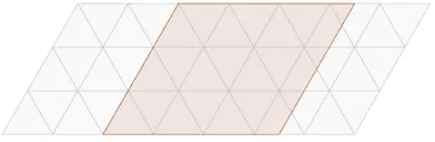
In Figure 31, we see the parallelogram region. We see its upper, lower, and left edges laying

upon the cell borders; the right edge however does not. No matter how one may shift this region

on the grid, at least one edge will not lay on the borders or altitudes of cells simultaneously with

all others. Regions like thisnon-calculable.

Theorem 17. If there is no combination of parity vectors that add up to a region’s parity measurement then there is no proper solution.

Proof. Assume there is a proper solution for a given region. If it exists then we would be able to measure the parity vector of each polydrafter within the region. Adding each drafter’s parity

vector would then result in the same parity vector of the region itself. If we can’t find a combination

that creates the desired parity vector, then no proper solution exists for the region.

Regions which are non-calculable have no parity vector defined for them. This allows for

the following lemma.

Lemma 18. A non-calculable region will have no with-the-grain solution.

If we perform a parity measurement upon the trapezoidal region in Figure 32, shown below,

it has a parity vector ofh6, 0, 0 i. Looking through all combinations of manipulating our 14

tridrafter’s parity vectors, there are some which do create a result ofh6, 0, 0i. This doesn’t mean

that there are solutions that are properly connected; it simply doesn’t rule out the possibility. (the

method to find these combinations are explained in a later section) Theoretically, we may create

more parities using similar processes that created the three used here. Often though the values

will change with the same pattern showing no new relationships when rotating and/or reflecting,

or the values have no recognizable cyclic pattern. These new parities are then often redundant or

too complex to be of inherent use.

Figure 32 shows the trapezoid and a home-plate region. Both are calculable and colored to

assist in finding their parity vectors to aid in analysis.

IV.2

A Tri-Coloring Analysis of the Tridrafters

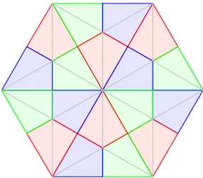
A second method, new in design, is thetri-coloringmethod. As the name may suggest, we use three colors to give values to our tridrafters based upon these three colors. This gives us three

values similar to the three variant parity method but at the same time; one for each color. We take

the equilateral triangles and each of them have all three altitudes placed creating six congruent

30◦-60◦-90◦triangles ormini-drafters. We then take the six triangles and color them in pairs such that the triangles with their 30◦ angles in the same corner are colored the same as shown in Figure 33. When the equilateral triangle is pointed upwards: the two in the upper corner are

colored red, the two in the left corner are colored blue, and the two in the right corner are colored

green. The downward cells are 180◦ rotations of the upward cells. Looking back at the cells, we see we have three kites within each cell made up of two right triangles which are given a

value of 1, giving the entire kite a value of 2. We also represent these in a vector form with three

components.

Figure 33:Tri-coloring grid

Following the same process to determine values with respect to parity, we can do the same

for tri-coloring. Here,xwill represent the number of red mini-drafters covered by the drafter,y

for the blue, andzfor the green.

Definition 13. LetRbe a figure (polydrafter, region, etc.). We definetas the function that takesR

and maps it to the 3-dimensional vectorhx,y,ziwherex,y, andzare the tri-coloring values as

T1’s tri-coloring vectort(T1), in it’s shown position, would beh3, 2, 4i. Figure 34 provides a visual.

Figure 34:T1’s drafter positions on tri-coloring grid

Just as it was with ourparityprocess, when performing actionsσorτ, the vector’s

compo-nents are altered. Unlike the parity measuring though, our numbers remain constant and shift

their positions within the vector rather than being negated.

Theorem 19. Performing actionσ(P)will alter the tri-coloring vector’s measurement fromhx,y,zito

hz,x,yi. Given a polydrafter T with t(T) =hx,y,zi, t(σ(T)) =hy,z,xi.

Proof. Any polydrafter may be measured through a similar process relative to Figure 34; here count the number of colored half-cells and add them to determine the appropriate colored values.

If the polydrafter is rotated 60◦ then all drafters composing the polydrafter rotate 60◦. After realigning the drafter to its new orientation; red values now rest in a green area, blue values now

rest in a red area, and green values now rest in a blue area. This causes each component of the

vector to shift to the left.

Theorem 20. Given a polydrafter T with t(T) =hx,y,zi, t(σ2(T)) =hz,x,yi.

Proof. Any polydrafter may be measured through a similar process given relative to Figure 34; here count the number of colored half-cells and add them to determine the appropriate colored

now rest in a green area, and green values now rest in a red area. This causes each component of

the vector to shift to the left twice.

Theorem 21. Given a polydrafter T with t(T) =hx,y,zi, t(τ(T)) =hx,z,yi.

Proof. Any polydrafter may be measured through a similar process relative to Figure 34; here count the number of colored half-cells and add them to determine the appropriate colored values.

If the polydrafter is reflected vertically then all drafters composing the polydrafter are reflected

as well. The red values then still rest in a red area, blue values now a green area, and green

values now in a blue area. This causes the second and third components of the vector to swap

locations.

Corollary 21.1. The tri-coloring vector of any polydrafter T can only be altered to one of six forms when performing actionsσandτ: its originalhx,y,zi,hy,z,xi,hz,x,yi,hx,z,yi,hy,x,zi, orhz,y,xi.

Note that a full upward and downward cell will always have 2 red mini-drafters, 2 blue

mini-drafters, and 2 green mini-drafters which will always result in a tri-coloring vector of

Table 2:Color values by position

Orientation x y z

1 1 2 0

2 1 0 2

3 2 0 1

4 0 2 1

5 0 1 2

6 2 1 0

7 1 2 0

8 1 0 2

9 2 0 1

10 0 2 1

11 0 1 2

12 2 1 0

We can give a tri-coloring vector to any region just as we gave a parity vector before.

The trapezoidal region we’ve worked with is composed of 21 full cells. As each cell has the

tri-coloring vector ofh2, 2, 2i, the region has a tri-coloring vector ofh42, 42, 42i. Note that like with

the parity vector, no tri-coloring vector can be given to a region such as the rhombus shown in

Figure 31.

Just as we have multiple combinations to create theh6, 0, 0ivector from our parity

measure-ments, we have multiple combinations that create the resultant vectorh42, 42, 42i. This method, on

its own, also fails to prove the observed conjecture.

IV.3

Combining Measurments

Definition 14. Thehexcombis the six component vectorha,b,c,x,y,ziwherea,b, andc are the values from parity measuring andx,y, andzare the values from tri-color measuring.

When we perform theσorτaction, we simply apply the individual rules fora,b, andc,

and then the individual rules forx,y, andzas they have been explained previously. Table 1 shows each of the 14 tridrafters, labeled with respect to the tridrafter shapes listed in figure 13, and their

measurments as itsidentityform, I.

The identity position, I, is arbitrary. One may create a table similar to Table 3 gathering the

Table 3:Ivalues

I(Tn) a b c x y z

T1 1 1 -1 3 2 4

T2 1 1 -1 3 2 4

T3 1 3 1 5 2 2

T4 1 1 -1 1 2 6

T5 1 1 3 3 2 4

T6 1 1 -1 3 2 4

T7 1 1 -1 3 2 4

T8 1 1 3 3 2 4

T9 1 1 -1 3 2 4

T10 1 1 -1 1 3 5

T11 1 1 3 1 2 6

T12 1 3 1 3 3 3

T13 1 1 3 1 3 5

T14 1 1 -1 3 2 4

Tables 5 through 16 located in the appendix show tables like the one above for all 12

position’s values (starting with this for Table 5) for all 14 drafters.

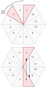
Jost and Maor depict actions simply; through the use of a pictorial chart showing how all six

portions of an equilateral triangle are formed by drawn altitudes. [6] A useful tool to this problem

would be a table that shows the resultant position a shaped ends up in when we take any two

actions with repetition allowed. We have a total of 12 actions that describe what position the shape

is in with respect to the standard position it starts in.

1. σm(Tn): The tridrafter,Tn is rotated 60◦mtimes, 0≥m≥5. 2. τ(Tn): The tridrafter,Tn is reflected vertically.

If we take any two random actions, repetition allowed, and perform them on any polydrafter,

possible pair of ordered actions and what position they result in. To find the resultant position

of combining two actions, match the row to the first action performed and the column to the

second action performed. The main purpose of this table is to demonstrate that any combination

or actions will always result in one of the twelve originally defined positions; implying that this

set of actions is closed.

For example,σ4(τ(T4))is takingT4in its initial positionIfrom its position and performing a reflection followed by a total of four rotations of 60◦. The resultant position can be found in the table in the seventh row and the fifth column; the result beingσ2τ. You can also reason from

this that reflecting a polydrafter followed by rotating it four times is the same as rotating the

polydrafter twice and then reflecting it.

Table 4:Two actions

Action I σ σ2 σ3 σ4 σ5 τ στ σ2τ σ3τ σ4τ σ5τ

I I σ σ2 σ3 σ4 σ5 τ στ σ2τ σ3τ σ4τ σ5τ σ σ σ2 σ3 σ4 σ5 I στ σ2τ σ3τ σ4τ σ5τ τ σ2 σ2 σ3 σ4 σ5 I σ σ2τ σ3τ σ4τ σ5τ τ στ σ3 σ3 σ4 σ5 I σ σ2 σ3τ σ4τ σ5τ τ στ σ2τ σ4 σ4 σ5 I σ σ2 σ3 σ4τ σ5τ τ στ σ2τ σ3τ σ5 σ5 I σ σ2 σ3 σ4 σ5τ τ στ σ2τ σ3τ σ4τ τ τ σ5τ σ4τ σ3τ σ2τ στ I σ5 σ4 σ3 σ2 σ στ στ τ σ5τ σ4τ σ3τ σ2τ σ I σ5 σ4 σ3 σ2 σ2τ σ2τ στ τ σ5τ σ4τ σ3τ σ2 σ I σ5 σ4 σ3 σ3τ σ3τ σ2τ στ τ σ5τ σ4τ σ3 σ2 σ I σ5 σ4 σ4τ σ4τ σ3τ σ2τ στ τ σ5τ σ4 σ3 σ2 σ I σ5 σ5τ σ5τ σ4τ σ3τ σ2τ στ τ σ5 σ4 σ3 σ2 σ I

Looking closely, we see that this is the dihedral group with 12 elements,D6. We will take it and make two more. These will be copies of Table 4 with all actions that cause the same resultant

for the tri-coloring vectors.

Table 5:Two action parity

Action I σ σ2 σ3 σ4 σ5 τ στ σ2τ σ3τ σ4τ σ5τ

I I σ σ2 σ3 σ4 σ5 τ στ σ2τ σ3τ σ4τ σ5τ

σ σ σ2 σ3 σ4 σ5 I στ σ2τ σ3τ σ4τ σ5τ τ σ2 σ2 σ3 σ4 σ5 I σ σ2τ σ3τ σ4τ σ5τ τ στ

σ3 σ3 σ4 σ5 I σ σ2 σ3τ σ4τ σ5τ τ στ σ2τ σ4 σ4 σ5 I σ σ2 σ3 σ4τ σ5τ τ στ σ2τ σ3τ

σ5 σ5 I σ σ2 σ3 σ4 σ5τ τ στ σ2τ σ3τ σ4τ τ τ σ5τ σ4τ σ3τ σ2τ στ I σ5 σ4 σ3 σ2 σ

στ στ τ σ5τ σ4τ σ3τ σ2τ σ I σ5 σ4 σ3 σ2 σ2τ σ2τ στ τ σ5τ σ4τ σ3τ σ2 σ I σ5 σ4 σ3

σ3τ σ3τ σ2τ στ τ σ5τ σ4τ σ3 σ2 σ I σ5 σ4 σ4τ σ4τ σ3τ σ2τ στ τ σ5τ σ4 σ3 σ2 σ I σ5

Table 6:Two actions tri-coloring

Action I σ σ2 σ3 σ4 σ5 τ στ σ2τ σ3τ σ4τ σ5τ

I I σ σ2 σ3 σ4 σ5 τ στ σ2τ σ3τ σ4τ σ5τ

σ σ σ2 σ3 σ4 σ5 I στ σ2τ σ3τ σ4τ σ5τ τ

σ2 σ2 σ3 σ4 σ5 I σ σ2τ σ3τ σ4τ σ5τ τ στ

σ3 σ3 σ4 σ5 I σ σ2 σ3τ σ4τ σ5τ τ στ σ2τ

σ4 σ4 σ5 I σ σ2 σ3 σ4τ σ5τ τ στ σ2τ σ3τ

σ5 σ5 I σ σ2 σ3 σ4 σ5τ τ στ σ2τ σ3τ σ4τ

τ τ σ5τ σ4τ σ3τ σ2τ στ I σ5 σ4 σ3 σ2 σ

στ στ τ σ5τ σ4τ σ3τ σ2τ σ I σ5 σ4 σ3 σ2 σ2τ σ2τ στ τ σ5τ σ4τ σ3τ σ2 σ I σ5 σ4 σ3 σ3τ σ3τ σ2τ στ τ σ5τ σ4τ σ3 σ2 σ I σ5 σ4

σ4τ σ4τ σ3τ σ2τ στ τ σ5τ σ4 σ3 σ2 σ I σ5 σ5τ σ5τ σ4τ σ3τ σ2τ στ τ σ5 σ4 σ3 σ2 σ I

Again, table 4 has the same symmetry as the dihedral groupD6. What this tells us is that no matter which of our original 12 actions we take and combine with any other action, we never

end up with a result that couldn’t be made with a single one of those original actions in the first

place. Applying each action once to each drafter and measuring its hexcomb yields all possible

forms the polydrafter may be expressed in.

Finding the hexcomb of a specific region is simply combining the parity and tri-coloring vectors

for said region together.

With the knowledge of our 12 possible single actions already relaying the results of any

com-bination of actions, one is able to come to the question "What are all possible resultsha,b,c,x,y,zi with all 14 pieces being measured in every possible position?". As there are 14 pieces with 12

possible positions there are 1214or 56, 693, 912, 375, 296 potential unique hexcombs.

Using Mathlab and the RIT Cluster Network, all possible results were calculated. The

V.

M

easuring

S

olutions

V.1

Hexcombs of Solutions

Each of the 75 convex shapes that can be created using the 14 tridrafters potentially have a hexcomb

to describe it. The following procedure explains how the potential hexcombs were found.

1. Take the outline of the region and place it so at least one side conforms to the triangular

grid.

2. Move the outline around such that as many sides as possible conform to the triangular grid

or the altitudes of the triangles that make up the grid simultaneously.

3. If it is possible to have all sides conform simultaneously, find the hexcomb that defines the

shape.

4. If it is not possible to have all sides conform simultaneously, the shape has no parity or

tri-coloring vector, and thus cannot be given a hexcomb.

Like the rhombus from Figure 31, if the entirety of the region can’t conform to cell borders,

the region can not be assigned a hexcomb value as it has no parity vector or tri-coloring vector to

describe it.

For those regions that can be placed upon the grid such that a hexcomb can be measured,

we find it. We find the hexcomb with the following procedure.

1. Place the region upon the grid such that all sides of the shape are bound by the triangular

grid or the trangle’s altitudes.

2. Color all equilateral triangles that point upwards black.

(a) Each black cell has a value ofh2, 0, 0, 2, 2, 2i

3. Color all equilateral triangles that point downwards grey.

4. Color all right triangles created fro