A stochastic optimization model for real-time operation of reservoirs using uncertain forecasts

WATER RESOURCES RESEARCH, VOL. 20, NO. 8, PAGES 1039-1046, AUGUST 1984

A Stochastic

Optimization

Model for Real-Time Operation

of Reservoirs

Using Uncertain Forecasts

BITHIN DATTA1

Department of Civil Engineering, University of Washington

MARK H. HOUCK

School of Civil Engineering, Purdue University

A real-time operation model primarily useful for daily operation of reservoirs is developed. This model is based on a chance constraint formulation and assumes a particular form of the linear decision rule. It uses the conditional distribution function (CDF) of actual streamflows conditioned on the forecasted values. These CDF's are constructed by incorporating the statistical properties of forecast errors for different time steps. The objective considered is the minimization of weighted probable deviations from storage and release targets. These weights are surrogates for th e actual loss functions, and the probable

deviations are functions of the reliability•levels specified in the model. With the use of target values for release and storage, this model is capabl e of using a release policy that is a subset of a seasonal policy and overcomes the myopic (short-sighted) nature of operation. Simulation of actual operation, using this model for a hypothetical reservoir, demonstrates the feasibility and efficiency of this approach. This

model is shown to be applicable for a system of reservoirs. The restrictions associated with the use of a

linear decision rule are shown to be invalid for this model.

INTRODUCTION

Fundamental distinctions exist between optimization models intended for planning and those intended for short-

term or real-time operation of reservoirs. These distipctions

are based on the type of inførmation provided to these models

and the goals and objectives to be satisfied. Long-term plan-

ning models should incorporate seasonal hydrologic data and long-term benefit functions. Long-term planning targets are obtained as outputs from these models.

F6r real-time

operation,

where

decisions

are

made

relatively

quickly and are based on short-term information, decisions

regarding release should be dependent ,on the starting reser- voir storage, penalities for deviations from planned targets, and short-term forecasts. When dealing with very small time

steps such as 1 hour, the hydrologic forecasts have very little

uncertainty,

and it should

be possible

to use

these

forecasts

as

deterministic

inputs

to an optimization

model.

This paper

does not address the problem of minute-by-minute operation,

however. The model described here emphasizes the incorpor-

ation of uncertainties inherent in short-term (for example, 12- hour, 1-day, 3-day etc.) hydrologic forecasts into the decision- making process. Reliability measures of the system per- formance are developed on the basis of the forecasts' errors or

hydrologic uncertainties.

Background

Some

of the past

research

dea[•gg

with real-time

operation

of reservoirs

is reported

•n Ja•!•n and

Wilkinson

[1972],

Windsor

[1973],

Trott

ana

¾eh

t73-1, chu

and

¾eh

[1978],

Yeh et al. [1979], Toebes and Rukvichai [1978], Fults and Hancock [1972], Becker and Yeh [1974], Becker et al. [1976],

• Presently at Water Resources Management Laboratory, Engi-

neering Experiment Station, University of Arkansas.

Copyright 1984 by the American Geophysical Union. Paper number 4W0694.

0043-1397/84/004W-0694505.00

Tennessee

Valley

Authority

[1974t'i

Houck

[198•:J],'Shane

and

Gilbert

[1980],

•aziciail

et al. [1983],

and

Siavai•'dason

[1976].

Useful

di•ussion

of the approaches

reported

in some

of

these papers can be found in Yeh [1982] and in Toebes and

Rukvichai [1978]. Sigvaldason [1976] proposed a simulation

model

for the real-time

operation

of a multireservoir

•system

by using a penalty function approach. Yazicigil et al. [1983] extended this simulation approach and presented a unified

screening and simulation approach for the Green River Basin

reservoir system. Houck [1981] commented on the s•nsitivity of the penalty functions used for real-time operation and pro-

posed a suitable form of the objective function to achieve an

operation policy that conformed more closely to a hypotheti- cal, ideal operation policy. Shane and Gilbert [1980] proposed the combined use of simulation and optimization methods for

a weekly time-step reservoir system scheduling model for the Tennessee Valley reservoir system.

No specific

review

of li{erature

related

to the

application

of

tems

Planning

or operation

is made

here.

Interested

readers

may refer to Hogan et al. [1981], ReVelle et al. [1969], Joeres et al. [1981], Houck and Datta [1981], Loucks and Dorfman

[1975], and Stedinger et al. [1983].

In this paper a real-time operation model is proposed that uses chance constraints, assumes a linear decision rule (nonre- strictive) as an operation policy, and incorpoi'ates the prob- abilistic.nature of real:time forecasts by considering the distri-

butionS:of

actual stre•:•mflow

volumes

conditioned

on fore-

casted values. The cOtiditional distribution functions are con- structed from the distribution of the errors associated with such forecasts. The objdCtive of the model is the minimization

of w. eighted probable deviations from storage and release tar-

gets

obtained

from a planning

model.

These

weights

are surro-

gates for the actual loss functions, and the probable deviations are functions of the reliability levels specified in the model.

1040 DATTA AND HOUCK' MODEL FOR REAL-TIME OPERATION OF RESERVOIRS

shown to be applicable to a system of reserviors. The re- strictions associated with the use of a linear decision rule are

shown to be invalid for this model.

DEVELOPMENT OF THE MODEL

Formulation of this model consists of two distinct steps. The first step involves the statistical evaluation of available forecasts for the inflows to the reservoir. The second step in-

volves the formulation of the optimization model incorpor-

ating the statistical characteristics of the forecast errors.

Incorporation

of Hydrologic

FOrecast

Errors

The model to be developed requires streamflow forecasts and information on the reliability of these forecasts: The nec- essary statistical analysis includes the determination of the

errors involved in forecasting the streamflow values for various time steps. These forecasts may be based on a sto- chastic model and/or a conceptual model. It is assumed that the errors have certain statistical properties that remain in-

variant for the time horizon for which the forecasts are made

and for the time horizon of the optimization model.

One method of quantifying the reliability of forecasts begins

with the estimation of the fractional error e for a given time

interval:

actual streamflow minus forecasted streamflow

e=

forecasted streamflow

This definition implies that the errors in forecasis are normal-

ized

by the magnitude

of respective

forecasts.

This

definition

may be modified, and the error considered may be assumed to be independent of the magnitude of forecasts for different cases, especially when a time series model is being used for forecasting and where the errors, as a requirement, are white

noise.

From the existing streamflow records and the available

forecasted streamflows for a portion of the record it is possible

to construct the cumulative distribution function of e. This

can be used to define the cumulative distribution function of the actual inflow, Rt(f•), during a period of t days with a

forecast offt because

Rt(ft) = eft + ft

This distribution function is the basis of assessing the reliabil- ity that the actual streamflows will remain within given

ranges. The following optimization model is then formulated t

by utilizing this information. T

The

Optimization

Model

TAR

This

optimization

model

utilizes

the

forecasted

streamflow

T R•(t,

•

volumes and the distribution function of the actual stream-

flows

conditioned

on

forecasted

values.

The

explicit

objective

Xmin(t

' t')

target values for release and storage for the time horizon of the model. The implicit objectives are to satisfy given lower and upper bounds of storage and release with specified relia- bilities. The following notation is used in the model.

bt(f,) decision variable for the period between the be- ginning of day 1 and the beginning of day t + 1, conditioned on forecasted streamflow equal to f,

during the same period, m3;

CAP capacity of reservoir, m 3;

Dr(t,

•

release

deficit

from target

value

for the period

be-

tween the beginning of day t + 1 and the beginning

of day œ

+ 1, m3;

Dts storage

deficit

from target value at end of day t,

m 3 ß

Er(t,

•

release

excess

from

target

value

for the period

be-

tween the beginning of day t + 1 and the beginning of day [ + 1, m3;

E, s storage excess from target value at end of day t, m 3 ß

f, forecasted

streamflow

for the period

between

the

m 3 ß

Ft( ) cumulative

distribution

function

of R,(f•);

Ft-•( ) inverse

cumulative

distribution

function

of

K(t, •

a tolerance

limit placed

on the deviation

of release

commitments obtained as solutions on a particular

day for release

in the period

between

the beginning

tained

from

the solution

on the previous

day,

m3;

Pr probability of;

Pt

sd a constant

equal

to the weight

specified

in the ob-

jective function for the storage deficit from the

target

value

at end

of day t;

ptSe a constant equal to the weight specified in the ob- jective function for the storage excess from the

target value at end of day t;

pt?d a constant

equal

to the weight

specified

in the ob-

jective function for the release deficit from the

target

release

in the period

between

the beginning

of day t + 1 and the beginning

of day [ + i;

pt• re a constant equal to the weight specified in the ob-

jective

function

for release

excess

from

the target

release in the period between the beginning of day

t + 1 and the beginning

of day [ + 1;

Rt(f ,) streamflow between the beginning of day 1 and the

beginning of day t + 1, conditioned on forecasted

streamflow equal to f, during the same time period,

m 3 ß

S• initial storage at beginning of day 1, m3;

Smin minimum storage allowable, m3;

St+ x(f•) storage at the beginning of day t + 1, conditioned on forecasted inflow equal to f, in the time period

from the beginning

of day 1 to the beginning

of

day t + 1, m 3;

tth day;

time horizon considered, days;

target storage during the time horizon considered, m 3 ß

target release between the beginning of day t + 1 and the beginning of day [ + 1, m3;

minimum allowable release for the period between the beginning of day t + 1 and the beginning of

day [ + 1, m3;

Xt(f•) release between the beginning of day 1 and the

beginning of day t + 1, conditioned on forecasted

streamflow equal to f, in the same time period, m3;

X(t, [)= X•(J•)- Xt(f,

) release

between

the beginning

of

day t + 1 and the beginning

of day [+ 1, con-

ditioned

on forecasted

streamflow

equal

to f• in the

DATTA AND HOUCK' MODEL FOR REAL-TIME OPERATION OF RESERVOIRS 1041

The explicit form of the objective function considered in this model is the minimization of the weighted sum of maximum

probable deviations from storage and release targets. These

maximum probable deviations are defined by the reliabilities with which these deviations are not to be exceeded. A linear equivalent of this objective function suitable for inclusion in a linear program is

T

Minimize

D = • (Pt

sd

* Dts

q- Pt

se

ß Et

s)

t=l T-1 T

q- E

E [Pti

rd

* Dr(

t, t') + Pti

re

ß Er(t, t)]

(1)

t=0 i=t+ 1

The values of at s and Et s are deficit and excess storages at

the end of day t, and the values

of Dr(t, t• and Er(t, t• are the

deficit and excess releases for the period between the be-

ginning of day t q- 1 and the beginning of day [ q- 1. The appropriate constraints to define the excess and deficit storage values are

S,+,(ft) = TAR + E, •- D, • (2)

D/> 0 (3)

œ/_> o (4)

Use of expected values in the objective function of a real-

time operations model is restrictive in the sense that it requires

utility functions that reflect how prone or averse the decision

makers are to risk. Though theoretically plausible, in practice, utility functions are difficult if not impossible to construct because of the presence of multiple objectives, conflicting in- terests, and multiple decision makers. Therefore, the expected value criterion is not used in the objective function of this model.

The decision rule used assumes the release from the be- ginning of day 1 to the beginning of day t + 1, conditioned on

forecasted streamflow equal to f,, to be a linear function of the

storage at the beginning of day 1:

x,( f ,) = s, - b,( f ,) (5)

The value of the decision variable bt(ft) will be chosen to optimize the objective function.

Substituting the decision rule Xt(f0 = S• - bt(ft) in the con- tinuity or mass balance equation, the following equations are obtained:

St+

•(f,)= S• + Rt(f,)- Xt(f,)= Rt(f,) + bt(f,)

(6)

t=l, 2 .... ,T

X(t, œ)

= X•(f•)- Xt(ft

) = bt(ft

) - b•(f•) (7)

t= 1,2,..., T- 1 t<œ<T

X(0, 1)= S, - b,(f,) (8)

The chance constraints imposed, considering Rt(f•) as a random variable, are

1. The probability that the storage at the beginning of each period is greater than or equal to a specified value, Smi,,

must equal or exceed a specified minimum value fi(t).

Pr[St+ •(ft) > Smin] >' •(t) (9)

or

Pr[Rt(f•) < Smi n -- bt(ft)] • 1 - fi(t) (10)

or

Ft[Smi n - bt(ft)] • 1 - fi(t) (11)

or

Smi n -- bt(ft ) •-• Ft-'[1 - fi(t)] t= 1, 2, ..., T (12)

2. The probability that reservoir storage at the beginning of each period will be less than the reservoir capacity CAP must equal or exceed a specified value 7(0. Apparently this equation means that there may be a nonzero probability of

the reservoir capacity being exceeded. In reality this means

that there will be a spill equal to the amount by which the

capacity is exceeded.

Pr[St+ ,(f•) _< CAP] _> 7(t) (13)

or

CAP - bt(ft)

> Ft -' [7(t)]

t = 1, 2 ... T

(14)

3. The probability that the release between the beginning

of day t + 1 and [ + 1 is greater

than

the minimum

specified

value

Xmin

(t, œ)

for that period

must

equal

or exceed

a speci-

fied minimum value •(t, D.

Pr[X•(f•)- Xt(ft

) > Xmin(t

, œ)]

• •(t, t")

(15)

or

Pr[bt(ft)- b•(fO

> Xmin(t,

/)] > •(t, D

(16)

The quantity

X(t, t') is used

rather

than daily releases

because

the model assumes that the releases for shorter time periods are subsets of longer time period releases. The high degree of statistical dependence between inflows over these periods is accounted for in this way. Because bt(f) and b•(J•) are not

random variables for a particular solution, •(t, œ) is assumed equal to 1, so that the above constraints reduce to

bt(ft

) -- b•(f•)

• Xmin(t

, œ)

(17)

t=l, 2 .... ,T-1 t<[<T

S, - b,(f,) > Xmin(0 , 1) (18)

Constraints 17 and 18 imply that the probabilities of meeting the release constraints are dependent on the probabilities of

meeting the constraints on storages. These constraints ensure

that bt(f,)

_>

b•(f•),

t </'. If these

constraints

were

not specified,

it could have been possible that the releases specified by Xt(f,)

would not be monotonically increasing functions of t. This is because different forecasts and error distributions are used for different values of t(t = 1,..., T).

4. In order to account for the objective function given by equation (1), constraint sets that specify the maximum prob- able deviations from storage targets as a function of the speci- fied reliability levels must be incorporated. Constraints serving

this purpose may be specified as

Pr[St+ •(ft) > TAR- Dt •] > 6(0 (19)

or

or

Pr[Rt(ft ) + bt(ft ) > TAR - Dt •] > 6(0 (20)

1042 DATTA AND HOUCK: MODEL FOR REAL-TIME OPERATION OF RESERVOIRS

Similarly, for storage excesses from the target value, Pt[St+ •(ft) -• TAR + ES(t)] •_ #(t)

or

(22)

TAR + ES(t)- bt(ft ) >_ F,-'[/•(t)] (23) t=l, 2 ... T 5. Because of this model's formulation, the release may be met with 100% probability, provided there is enough water in storage. Constraints that specify the deficit or excess releases to be incorporated in the objective function may be stated as

X(t, • _• TRe(t

, •- D'(t, •

(24)

or

Tee(t,

h - b,(f,)

+ b•(f•)_•

D'(t, t")

t= 1,2,..., T-1

(25)

t<i'_<T

and

Also

or

and

Tea(O, 1) - S • + b • (f•) _< D'(O, 1) (26)

X(t, h •- Tee(t,

h + E'(t, h

o,(f,)- o,(f,)-

h -< e'(t, h

t=l, 2 ... T-1

(28)

t<i'_<T

S, - b,(f•)- Tee(O, 1) _< E'(O, 1) (29) 6. The primary function of this model is predictive in nature; it may therefore be desirable that the proposed release policy for the next several days not change too dramatically as the release policy is updated during these several days. By limiting the changes in release policy from one day to the next, the flexibility to respond to streamflow forecast changes is reduced, but the ability to plan activities dependent on the release policy is enhanced. To restrict the deviations between the releases predicted for the same day or days by a previous solution of the model and a current solution of the model, these constraints may be added:

X(t, t")

_• XO(t,

t")

+ K(t, t")

X(t, h -• X•( t, h- K(t, h

XO(t,

• denotes

the optimum

value

of the predicted

release

between the beginning of day t q- 1 and the beginning of day

[ q- 1 obtained

as solution

to the model

on the previous

day.

In practice the value of t may be restricted to 1 or 2 days, and

the value of [ may be restricted

to t q- 1 or t q- 2 in these

constraints. Real-time forecasts are quite accurate only for a

lead time of 1 or 2 days, and restricting the operation policy to

a function of the policy based on forecasts of longer intervals may not be advantageous. Theoretically, however, these con- straints may be extended to cover the whole time horizon incorporated in a particular solution. Equivalent constraints using the linear decision rule may also be stated as:

b,(f,)- b,(f•)

_• X•(t, h + K(t, h

and

b,(f,)- b,(f•)

•_ X•(t, h - K(t, h

Therefore, this model consists of the objective function

(equation (1)) of minimizing the weighted sum of maximum probable deviations from target values of releases and storages for the time horizon of the model and a set of constraints (12, 14, 17, 18, 21, 23, 25, 26, 28, 29, 32-35) on performance re- quirements and the reliabilities with which these performance

criteria are to be met. The forecasts required for a single day's

solution of this optimization model are one time-step ahead

forecasts for time periods varying from 1 day to the time

horizon, which may be about 30 days. For each time step, different forecasting models may be used.

The objective function can be generalized to represent

better the actual penalty (opportunity cost) for deviations from the target values if ptsd, ptse, pt?a, and Pa re are defined as

functions instead of constants. The discounting factors for un-

certainties in the future may be assumed to be included in these functions. Using these functions instead of the weights (constants) as described before will require their definition in the constraint set and most likely require piecewise lin- earization because they will be nonlinear.

A further generalization of the objective is possible by al- lowing the reliability levels (fi, •, #) to be variables. Then the penalty functions would not only be functions of storage and

releases but also the reliabilities of those storages and releases.

Appropriate ranges of the cumulative distribution functions (CDF) of actual inflows conditioned on forecasted flows would have to be included (piecewise linearized) in the constraint set. One last extension of the objective would be to include the entire CDF's of storages and releases in the objective. This could be done approximately by defining several reliability levels (fi, •, #) between 0 and 1, determining the associated storage or release values, and approximating the remainder of

the CDF's.

In the next section the solution of the model will be dis-

cussed. The results of simulating the operation policies in a,

simulation model and motivations for some of the results will

be presented. It is hoped that this evaluation will help to make the assumptions in the model more clear.

SOLUTION OF THE MODEL

The first step in the evaluation of this model was to es-

tablish a hypothetical reservoir system for test purposes. In

practice the capacity of the reservoir will be a known value; however, because the reservoir system used in this evaluation is hypothetical, a single linear decision rule (LDR) model [Re-

Velle et al., 1969] with 12 seasons per year was used to find

the optimal capacity reservoir for the tests. The capacity re- quired for this hypothetical reservoir on the Tygert River in

West Virginia was 168.7 ß 106 m 3.

The next step in the model construction was the devel- opment of the forecasting models for different time steps Simple autoregressive models were used because the primary purpose of the optimization model presented here is not to evaluate the degree of accuracy of the forecasting models but

to utilize the information on the probable errors associated

DATTA AND HOUCK: MODEL FOR REAL-TIME OPERATION OF RESERVOIRS 1043

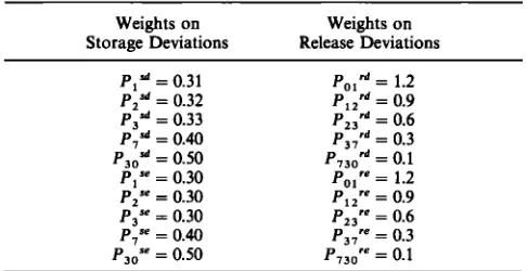
TABLE 1. Weights for the Objective Function

Weights on Weights on

Storage Deviations Release Deviations p•a = 0.31 Po• rd = 1.2 Pe a = 0.32 P•2 rd = 0.9 P3 sa = 0.33 P23 rd = 0.6

p?a = 0.40 P37 •a = 0.3

P3o s•t = 0.50 P73o n• = 0.1 p•se = 0.30 Po• •e = 1.2 p:s• = 0.30 P•:r• = 0.9 P3 se = 0.30 P23 re = 0.6 P7 se = 0.40 P37 re = 0.3 P3o se = 0.50 P73o re = 0.1

quences, different forecasting models may be developed for

different periods of the year.

The use of a linear decision rule, in the formulation of this model does not limit the solution space as it does in other models. S• is always a known quantity in an operation model, and therefore bt(ft ) can easily be replaced by S•- Xt(ft). Equation (12) would become

Smi n -- S 1 -•- St(f) • F t - '[-1 - fi(t)] (36)

It is now possible to find the optimum value of the decision

variables

X,(ft) and X(t, • by utilizing

(17).

This would

not be

the case with a planning model where S• is the initial storage at the beginning of a season and is to be treated as a random

variable. The limitiations often cited when a linear decision

rule (LDR) is used should not be valid here. This model should serve as an example where use of an LDR is not at all

restrictive.

The optimization model already presented is a generalized version of the model that was solved. To limit the compu- tational burden and to approximate more accurately the actual decision-making environment, the number of CDF's to be considered in a time horizon of T days was limited. For this particular study, according to the notation used, the values of t were restricted to 0, 1, 2, 3, 7, and 30 days. Values of [ were restricted to 1, 2, 3, 7, and 30 days only. Also for constraints 32 and 34 the value of t was restricted to 0, 1, and 2 days, while the value of [ was restricted to 1, 2, and 3 days. This means that in each subsequent solution of this model, at the beginning of each day, the release policy for the first three

days of solution was restricted to within some specified toler- ance limits of the predicted release as obtained by a solution of this model for the previous day.

This model also requires as inputs the storage volume at the

beginning of each day and the updated forecasts made on a

real-time basis at the beginning of each day. The releases and

storages for the second, third, and later days as specified by

the model are only used for forecasting purposes to predict the releases in future time periods. Only the solution for the first day is used for making actual releases. This preserves the real- time characteristics of the operation policy. The release policy

as predicted for a longer time period may be restricted by introducing bounds into the model to maintain the releases for a given time horizon or for a particular season within

some limits of the release commitment made from a planning

model.

The objective weights used in this example (Pt sd, ptse, pard,

and Pa re) were chosen arbitrarily (Table 1), keeping in mind

the general assumption that deviations from release targets are mare costly than an equal amount of deviation from a storage

target. Also the meeting of targets on the first day of a particu-

lar solution is relatively more important than that of subse-

quent days when the model inputs are actually updated and the operation policy revised.

The model was solved for varying initial conditions and different reliability levels. The operation policies obtained as solutions were tested by simulation of reservoir operation. The mathematical programming package XMP [Marsten, 1980] was used to solve the linear optimization models. Some of the

many variations of the model that were tested are given in

Table 2. These models were tested for an identical set of

streamflow data for a period of 30 days. The daily flows actu- ally occurring consisted of a series of high flows beginning on the third day and ending on the seventh day and a series of low flows beginning on the twenty-second day. Tables 2 and 3

summarize some of the results obtained.

Table 2 shows some of the variations of the model that were

tested. The columns in Table 2 specify the various levels of

reliabilities that were used in these models. In model A, only

the predicted values of streamflow were used. Therefore no reliability levels are applicable to this model. Model C speci- fies lower reliability levels as compared to model B for all the performance requirements except the storage deviation from target value in the 7- and 30-day periods.

Table 3 shows some results of solving these models at the beginning of each day for a 30-day period and of simulating

operating conditions by using actual streamflow volumes. Be- cause a series of high flows was considered for these examples,

the maximum volumes of the releases and storages were con-

sidered critical. It is evident from Table 3 that the maximum

storage attained during this period is largest in model A.

While model C results in a smaller value of excess deviation

from release target compared to model B, this occurs at the expense of attaining a higher storage excess than model B. This is because in model B the deviations from storage target

are restricted with higher reliabilities; however, in the process

of complying with this requirement, model B is forced to re-

lease a larger amount in order to be risk averse, i.e., to avoid

TABLE 2. Identification of Models With Different Inputs S 1 on

Model First Day, Xmi n (0, 1),

Identity 10 6 rn3 10 6 rn3 •1, •1 •2, •2 •3, •3 •7, •7 •30, •30 •I, ]A1 •2, ]A2 •3, ]A3 •7, •/7 •30, ]A30

A 85.57 2.44 --* • • •

B 85.57 2.44 0.90 0.85 0.85 0.75 0.70 0.85 0.85 0.80 0.70 0.70 C 85.57 2.44 0.75 0.75 0.75 0.70 0.70 0.75 0.75 0.75 0.75 0.75

CAP

= 168.70'106

m3;•

TRR(t,

•)= (;--t)*2*Xmin(O,

1); Smin

= 24.45'106

m3;

TAR

= 73.35'106

m3;

K(t, ;) - T•(t, ;); Xmin(t, t) = (t -- t)*Xmin(0, 1).

1044 DATTA AND HOUCK' MODEL FOR REAL-TIME OPERATION OF RESERVOIRS

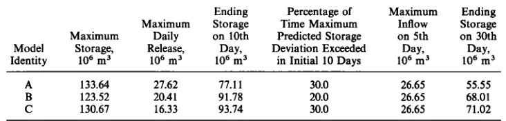
Model

Identity

TABLE 3. Simulation and Optimization Results for Different Models Ending Percentage of Maximum Maximum Storage Time Maximum Inflow Maximum Daily on 10th Predicted Storage on 5th Storage, Release, Day, Deviation Exceeded Day,

10 6 m 3 10 6 m 3 10 6 m 3 in Initial 10 Days 10 6 m 3

A 133.64 27.62 77.11 30.0 26.65

B 123.52 20.41 91.78 20.0 26.65

C 130.67 16.33 93.74 30.0 26.65

Ending

Storage

on 30th

Day,

10 6 m 3

55.55 68.01 71.02

bigger deviations in the future. Also the ending storages after 30 days (which is also the time horizon of the models for a particular solution) are nearer to the target value for models B

and C than for model A.

The inadequacy of using only predicted values as determin- istic inputs to the model is evident from the performance of

model A. Because this model simply uses the predicted values,

whenever high flows occur that differ appreciably from the predicted value, this model fails to recognize the higher per- centile values of future probable flows. This may result in very high deviations from the target values at certain stages. Also,

for a series of low flows, when not enough water is available to

meet the release targets during the last few days, the storage is depleted faster than with the other two models.

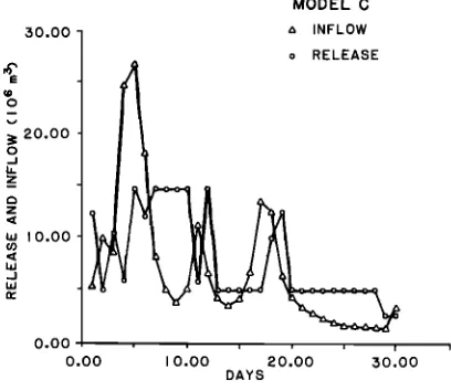
Figures 1-3 show release patterns obtained for these three

different models for an identical set of inflows. The fluctu-

ations in release volumes and storage volumes are most pro-

nounced in model A. Model C shows the minimum fluctu-

ation. With uncertain inputs, very large probable deviations from target values are guarded against in models B and (2 with higher reliabilities than model A. However, in model C the reliability levels are smaller than those of model B, and

therefore the critical values of minimum or maximum inflows

considered probable are less critical in model C than in model B. This may cause model B to release a higher volume than model C when a high flow is forecasted with identical initial

conditions.

Although many other variatons of the model with different inputs were considered, they are not reported here because it is not possible to reach definitive conclusions from limited examples. It is especially true when the performance of the model is very much dependent on the quality of the forecasts obtained from the forecasting model. This aspect is discussed in greater detail in Datta and Burges [1984]. These evaluations only show that the model is solvable, it gives sensible results

30.00

20.00

IO.OO

o.oo ,

o.oo

MODEL A

INFLOW o RELEASE

! i ! i

!

I0.00 20.00 30.00

DAYS

that are not counterintuitive, and these evaluations may be used to aid the judgment of the decision makers.

EXTENSION OF THE MODEL TO A SERIES OF RESERVOIRS

One of the strong points of the model presented is that it does not require complicated statistical manipulations such as convolution. Also, the linear programming algorithm can be used. This algorithm is simpler to use and substantially more versatile in many situations than other solution approaches such as dynamic programming. Therefore this model should be very useful if it can be extended to a series or network of reservoirs and still remain well within the range of compu- tational feasibility. The modification necessary to use this model for a system of reservoirs in series is presented here as an illustration. The objective function is now modified to

T N

Minimize

D = • • (P,t

sa

ß D,t

s + Pit

se

, E,t

s)

t=l i=1

T-1 T N

t=O i=t+l i=1

ß [Pm

'a ß O,'(t, [) + Piti

re

* Er(t,

[)]

(37)

Here the subscript i denotes reservoir i, with N reservoirs in series; for this example the reservoirs are numbered starting with 1 as the most upstream reservoir down to N as the most downstream reservoir. All the weights P may again be re- placed by actual or hypothetical loss or penalty functions for deviations from storage and release targets.

The continuity or mass balance equation is to be modified

to reflect that the total inflow into a reservoir is the uncon-

trolled inflow from the basin plus the release from an up- stream reservoir minus any withdrawal by the users between

reservoirs.

Therefore

X(t, [) should

now be replaced

by Xi(t ,

and Y:(t, [)' X•(t, [) refers

to that part of the release

(with-

MODEL B

30.00 a INFLOW

20.00

lO.00

0.00

o RELEASE

i i i i

0.00 I 0.00 20.00 30 O0

DAYS

DATTA AND HOUCK: MODEL FOR REAL-TIME OPERATION OF RESERVOIRS 1045

30.00

• 2o.oo

o

z

I

z

ta I0.00

MODEL C

_ A INFLOW

o RELEASE

0.00 .... ,

0.00

10.00

20•00

30.00

DAYS

Fig. 3. Releases and inflows for model C.

drawal) from reservoir i used in the control area of reservoir i;

and Y•(t,

• refers

to that portion

of the release

from reservoir

i

that enters the downstream reservoir i+ 1 as inflow. If the

losses

incurred

as a result

of deviations

frøm

a release

target

are due solely

to the withdrawal

from a reservoir

Xi(t, t), then

the deviations from the target withdrawal for a particular res-

ervoir

will be determined

by Tm•,(t,

t) - Xi(t, •.

For purposes of this illustration the release from a reservoir is assumed to arrive at the next downstream reservoir in the same day. Therefore, equations (5)-(7) are now given as:

Xit(ft) d- Yit(J•it) -- Sil -- bit(•it) (38) = s,, + x,,ff,,)-

+ Y•- •,t(f•- •,t) t - 1, 2 ... T

For i = 1 the previous equations become

i=2 ... N (39)

s,,,+ ,(A,)= s,, + R,,(A,)- x,,(A,)-

(4O)

and

Xi(t, • + ri( t, b = bit(fit)

- bif(fii)

(41)

t=l, 2 ... T--1 t<[<T i=1 .... ,N

Other constraints are to be suitably modified. For example, constraint 12 will now be given by

Smini

-- bit(fit)

- Yi- 1,,(f/-

1,t)

• Fit- '[1 - •(t)]

(42)

t=l, 2 ... T i=2,...,N Constraint 25 will now be given by

rm•,(t,

•- b,t(f•,)

+ b•(f•) + Y•(t,

• < D[(t, •

(43)

t=l, 2 .... ,T-1 t<[_<T i=l,...,N where Y•(t, D is defined by

Y•(t,

t)= Y•(f•)- Y•t(f/,)

(44)

In a similar fashion, all other constraints can be modified.

When there are reservoirs in series and parallel, similar con-

straints can be formulated.

SUMMARY AND CONCLUSIONS

This model is primarily for use as a real-time daily oper-

ation model. It must be solved at the beginning of each day, with updated forecasts, revised conditional distribution func-

tions of future streamflows, and the state of the system given

by the initial storage used as inputs. The objective of oper-

ation is to minimize the sum of penalties associated with devi- ations from target or Meal conditions for operations over a time horizon of several days to a month.

Theoretically, this model can be extended to shorter time-

steps such as hourly operations. However, hourly operations

are generally based on almost perfect forecasts of streamflows

and exact consumer demands for water supply and hydroelec- tri c power. Therefore in such a situation a deterministic opti- mization model, rather than a chance-constrained model, may

be more appropriate. Operation policies obtained as solutions

from monthly or seasonal models may be used as planning inputs to the daily operation model so that the release in a time horizon of 30 days can be specified by appropriately fixing the value of the decision parameter br(fr) with some tolerance.

The solutions obtained from the optimization model for

different input conditions were studied in a simulation of res- ervoir operation by using these policies. The results obtained give some insight to the working of this model. The simulation results may aid in the selection of appropriate levels of the

reliabilities to be specified by the decision makers for meeting different operational requirements. Also, using only the fore- casted values and ignoring the uncertain parts is a special case

of this model and may be acceptable when the probabilities of

system failures are very low. Some limitations of using only a forecasted value were demonstrated through model A.

The time horizon that should be considered in a particular

solution of this model must be decided on the basis of the

operational objectives. If the smaller time-step operation poli- cies are intended to be subsets of longer time-step operation

policies like seasonal or weekly time steps, the value of T should be appropriately specified.

This model was shown to be extendable to a system of

reservoirs. Also, the restrictions generally associated with the use of linear decision rules were shown to be invalid for this

model.

Acknowledgments. This material is based upon work supported by The National Science Foundation under grant CME-7916819. The authors are also grateful to the Purdue Research Foundation for their generous financial support under grant XR-0340.

REFERENCES

Becker, L., and W. W-G. Yeh, Optimization of real time operation of multiple reservoir system, Water Resour. Res., 10(6), 1107-1112,

1974.

Becker, L., W. W-G. Yeh, D. Fults, and D. Sparks, Operation models for the Central Valley Project, J. Water Resour. Plann. Manage. Div., Am. Soc. Civil Eng., 102(WR1), 101-115, 1976.

Chu, W. S., and W. W-G. Yeh, A nonlinear programming algorithm for real time hourly reservoir operations, Water Resour. Bull., 14(5),

1048-1063, 1978.

Datta, B., and S. J. Burges, Short-term single, multipurpose reservoir

operation: Importance of loss functions and forecast errors, Water Resour. Res., in press, 1984.

Fults, D. M., and L. F. Hancock, Optimum operations models for Shasta-Trinity system, J. Hydraul. Div., Am. Soc. Civil Eng., 98(HY9), 1497-1514, 1972.

1046 DATTA AND HOUCK: MODEL FOR REAL-TIME OPERATION OF RESERVOIRS

Houck, M. H., What is the best objective function for real-time opti- mal reservoir operation?, paper presented at International Sympo- sium on Real Time Operation of Hydrosystems, Univ. Waterloo, Ontario, Canada, 1981.

Houck, M. H., and B. Datta, Performance evaluation of a stochastic optimization model for reservoir design and management, Water Resour. Res., 17(9); 827-832, 1981.

Jamieson, D. G., and J. C. Wilkinson, River Dee research program, 3, A short-term control strategy for multipurpose reservoir systems, Water Resour. Res., 8(4), 911-920, 1972.

Joeres, E. F., J. S. Gunther, and H. M. Englemann, The Linear De- cision Rule (LDR) reservoir problem with correlated inflows, 1, Model development, Water Resour. Res., 17(1), 18-24, 1981. Loucks, D. P., and P. J. Doffman, An evaluation of some linear

decision rules in chance-constrained models for reservoir planning and operation, Water Resour. Res., 11(6), 777-782, 1975.

Marsten, R. E., The Design of the XMP Linear Programming Li- brary, MI$ Tech. Rep. 80-2, Univ. Ariz., Tucson, 1980.

ReVelle, C. S., E. Joeres, and W. Kirby, The linear decision rule in reservoir management and design, 1, Development of the stochastic model, Water Resour. Res., 5(4), 767-777, 1969.

Shane, M. R., and K. C. Gilbert, Weekly Time Step Reservoir System Scheduling Model, Part 1 and 2, report, Tenn. Val. Auth., Water Syst. Dev. Branch, Norris, Tenn., 1980.

Sigvaldason, O. T., A simulation model for operating a multipurpose multireservoir system, Water Resour. Res., 12(2), 263-278, 1976. Stedinger, J. R., B. F. Sule, and D. Pei, Multiple reservoir system

screening models, Water Resour. Res., 19(6), 1383-1393, 1983. Tennessee Valley Authority, Development of a comprehensive Ten-

nessee Valley Authority water resource management program,

paper presented at conference of International Institute for Applied

Systems Analysis, Laxenberg, Austria, July 1974.

Toebes, G. H., and C. Rukvichai, Reservoir systems operating policy•ase study, J. Water Resour. Plann. Manage. Div., Am. $oc. Civil Eng., 104(1), 195-209, 1978.

Trott, W. J., and W. W-G. Yeh, Optimization of multiple reservoir systems, J. Hydraul. Dit)., Am. Soc. Cit)il Eng., 99(HY10), 1865-1884,

1973.

Windsor, J. S., Optimization models for the operating of flood control systems, Water Resour. Res., 9(5), 1219-1226, 1973.

Yazicigil, H., M. H. Houck, and G. H. Toebes, Daily operation of a multipurpose reservoir system, Water Resour. Res., 19(1), 1-14,

1983.

Yeh, W. W-G., State of the art review: Theories and applications of systems analysis techniques to the optimal management and oper- ation of a reservoir system, Rep. UCLA.ENG-82-52, Univ. Calif., Log Angeles, 1982.

Yeh, W. W-G., L. Becker, and W. S. Chu, Real time hourly reservoir operations, J. Water Resour. Plann. Manage. Div., Am. Soc. Civil Eng., 105(WR2), 187-203, 1979.

B. Datta, Water Resources Management Laboratory, Engineering Experiment Station, University of Arkansas, Fayetteville, AR 72701.

M. H. Houck, School of Civil Engineering, Purdue University, West Lafayette, IN 47907.