Dynamics Based Control: An Introduction
Zinovi Rabinovich
Jeffrey S. Rosenschein
School of Engineering and Computer Science
The Hebrew University of Jerusalem
Jerusalem, Israel
Abstract
In this paper we introduce a novel approach to continual planning and control, called Dynamics Based Control (DBC). The approach is similar in spirit to the Actor-Critic [6] approach to learning and estimation-based differential regulators of classical control theory [12]. However, DBC is not a learning algorithm, nor can it be subsumed within models of standard control theory. We provide a general frame-work for applying DBC to discrete Markovian environments, and discuss the key differences between it and a popular alternative for this type of environment — Partially Observable Markov Decision Processes (POMDPs). We then show how a recently developed control scheme based on Extended Markov Tracking (EMT) [9, 10] can be seen as a suboptimal algorithm within the DBC framework, and discuss EMT’s limitations relative to the general DBC approach.
1
Introduction
Consider NASA engineers who encounter a serious problem: two spacecraft, while attempting to dock in orbit, keep crashing or whirring out of control. At first, control schemes and sensors are blamed for being inexact, and great efforts are invested in perfecting the precision of spacecraft positioning. Bizarrely, as precision improves, the problem perseveres and becomes even more violent. A surprising solution is proposed that finally solves the problem — reduce positioning precision. As long as orbits do not change too much, docking can be done using a simple funnel-like mechanism. This kind of problem, control of change over time, or in other words control of system dynamics, is what we describe in this paper.
The central idea behind Dynamics Based Control (DBC) is that if laws governing changes in a system, the system dynamics, are beneficial in some sense, then neither state estimation precision nor the state itself matter as much. These system dynamics, like the funnel of a vortex, will channel the system into the desired configuration. The target of a DBC algorithm would be to select actions in such a way as to create or simulate the beneficial dynamics.
Recalling our spacecraft docking scenario, applying Dynamics Based Control (DBC) would mean that instead of attempting to set the orbit position directly, one should ensure that it has the tendency to recover from deviations from an ideal orbit. This tendency would be the beneficial system dynamics, and it requires much less effort than precise positioning of a spacecraft. A similar effect is observed while driving a car (the “small corrections principle”); there is no attempt to precisely position the car in the middle of a car lane, but rather it is directed to return there.
The “small corrections principle” has another interpretation, that of classical control theory [12]. Control theory holds a concept of neighboring control. Should the system manifest itself in an ideal, noiseless way, the control signal (actions selected) would be clear. But if a (small) deviation in system state occurs, the control signal can be augmented by a small difference as well, usually proportional to the real or estimated state-difference, as observed in literature on linear systems [3, 12]. Though DBC uses terminology such as
system deviation, the focus is on the rules that govern the system, rather than on the system state itself.
The main principle of action selection in DBC can be split into two phases: dynamics estimation and
dynamics correction. Estimation can be done in numerous ways, starting from true system identification
DBC-type action selection is actually quite widespread. Consider, for example, color creation on a computer screen. Color perception by humans (that is, light frequency estimation) is based on three distinct receptors, each detecting a very specific frequency or hue. This is used in color monitors, where most of colors are not actually emitted by the screen. Instead, three sources of constant hue are tapped into, and a mixture is created that simulates for the human eye the required color. This scheme parallels the phases of
estimation and correction as performed by DBC.
Similar dual structure can be found in learning algorithms such as Actor-Critic algorithms [6]. A Critic estimates the value function, a system performance evaluator, while an Actor uses the estimation to refine its strategy. However, Actor-Critic algorithms are learning algorithms, and produce at the end a good value function estimate and the corresponding, usually static, strategy. The DBC framework by itself is not a learning algorithm, though it can be utilized in creating one (see below).
The rest of the paper is organized as follows. In Section 2 we provide a formal introduction to Dynamics Based Control, focusing especially on Markovian stochastic environments. This is followed in Section 3 by comparison to a classical control alternative for these environments — Partially Observable Markov Decision Processes (POMDPs). Section 4 demonstrates how recently introduced EMT-based control fits the DBC architecture under the Markovian assumption, and also exposes the limitations of the naive EMT-based control, as opposed to the general DBC framework. Section 5 provides some concluding remarks and directions for future developments of DBC.
2
Dynamics Based Control
Dynamics Based Control (DBC) specification can be broken into three interacting levels: Environment Design Level, User Level, and Agent Level.
• Environment Design Level concerns itself with the formal specification and modeling of the
envi-ronment. For example, this level would specify the laws of physics within the system, and set its parameters, such as the gravitation constant.
• User Level in turn relies on the environment model produced by Environment Design to specify the
ideal or beneficial system dynamics it wishes to observe. The User Level also specifies the estimation or learning procedure for system dynamics and the measure of deviation. In our spacecraft docking scenario these would correspond to specifications of self stabilization at an optimal orbit, and angular speed and radii difference evaluations.
• Agent Level in turn combines the environment model from the Environment Design level, and the
dynamics estimation and ideal dynamics specification from User Level, to produce a sequence of actions that create system dynamics as close as possible to the ideal one with respect to the deviation measure specified by the User Level.
As we are interested in the continual development of a stochastic system, such as happens in classical control theory [12] and continual planning [5], the question becomes how the Agent Level is to treat the deviation measurements over time. A classical approach would be to use expectation, to average over all possible system developments. However, we prefer to use a probability threshold alternative — that is, we would like the Agent Level to maximize the probability that the deviation measure will remain below a threshold.
Specific action selection would depend on system formalization. One possibility would be to create a mixture of available system trends, much like what happens in Behavior-Based Robotic architectures [1]. The other alternative would be to rely on the estimation procedure provided by the User Level, and utilizing the Environment Design Level model of the environment to choose actions so as to manipulate the dynamics estimator to believe that a certain dynamics has been achieved. Notice that this manipulation is not direct, but via the environment. Thus, for strong enough estimator algorithms, successful manipulation would mean a successful (i.e., beyond discerning via the available sensory input) simulation of the ideal or beneficial system dynamics.
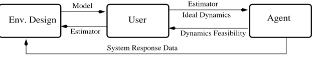
User
Env. Design Agent
Model
Ideal Dynamics Estimator
Estimator
[image:3.595.144.456.84.141.2]Dynamics Feasibility System Response Data
Figure 1: Data flow of the DBC framework
Extending upon the idea of Actor-Critic algorithms [6], DBC data flow can provide a good basis for the design of a learning algorithm. For example, the User Level can operate as an exploratory device for a learning algorithm, inferring an ideal dynamics target from the environment model at hand that would expose and verify most critical features of system behavior. In this case, feasibility and system response data from the Agent Level would provide key information for an environment model update. In fact, the combination of feasibility and response data can provide a basis for the application of strong learning algorithms such as EM [2, 8].
2.1
DBC for Markovian Environments
For a Partially Observable Markovian Environment, DBC can be specified in a more rigorous manner. In this case, the phases or levels of DBC can be seen as follows:
• Environment Design level is to specify a tuple< S, A, T, O,Ω, s0>, where:
– Sis the set of all possible environment states;
– s0is the initial state of the environment (which can also be viewed as a distribution overS);
– Ais the set of all possible actions applicable in the environment;
– Tis the environment’s probabilistic transition function:T :S×A→Π(S). That is,T(s0|
a, s)
is the probability that the environment will move from statesto states0under action
a;
– Ois the set of all possible observations. This is what the sensor input would look like for an outside observer;
– Ωis the observation probability function:Ω :S×A×S →Π(O). That is,Ω(o|s0, a, s)is the
probability that one will observeogiven that the environment has moved from statesto states0
under actiona.
• User Level, in the case of a Markovian environment, operates on the set of system dynamics described
by a family of conditional probabilitiesF={τ:S×A→Π(S)}. Thus ideal or beneficial dynamics can be described byq ∈ F, and the learning or tracking algorithm can be represented as a function
L:O×(A×O)∗→ F, that is, it maps sequences of observations and actions performed so far into
an estimateτ ∈ Fof system dynamics.
There are many possible variations available at the User Level to define divergence between system dynamics; several of them are:
– Trace distance orL1distance between two distributionspandqdefined by
D(p(·), q(·)) = 1 2
X
x
|p(x)−q(x)|
– Fidelity measure of distance
F(p(·), q(·)) =X x
p
p(x)q(x)
– Kullback-Leibler divergence
DKL(p(·)kq(·)) =X x
p(x) logp(x)
Notice that the latter two are not actually metrics over the space of possible distributions, but nev-ertheless have meaningful and important interpretations. For instance, Kullback-Leibler divergence is an important tool of information theory [4] that allows one to measure the “price” of encoding an information source governed byq, while assuming that it is governed byp.
The User Level also defines the threshold of dynamics deviation probabilityθ.
• Agent Level is then faced with a problem of selecting a control signal functiona∗
to satisfy a mini-mization problem as follows:
a∗
= arg min
a P r(d(τa, q)> θ)
whered(τa, q)is a random variable describing deviation of the dynamics estimateτa, created byL
under control signala, from the ideal dynamicsq. Implicit in this minimization problem is thatL
is manipulated via the environment, based on the environment model produced by the Environment Design Level.
3
DBC vs. POMDPs
The comparison of the DBC approach to classical control can be done via the comparison of DBC to Par-tially Observable Markov Decision Processes (POMDPs). Since POMDPs are a classical representative of the control theory of stochastic systems, and DBC has a well-formed formalization over Markovian envi-ronments, comparison between them will help illuminate the key features of the DBC approach.
Structurally, POMDPs can also be fitted into the three levels of the Environment Design Level, User Level, and Agent Level. Furthermore, one can assume that the Markovian environment model produced by the Environment Design Levels of both approaches completely overlap (see Table 1 for a structural comparison). However, the User and Agent Levels differ significantly. At User Level, instead of idealized system dynamics, the POMDP approach defines a reward functionr:S×A×S→Rto express preferences over different system transitions. POMDP at User Level also defines an optimality criterion, determining how the reward should be treated over time, e.g., discounted accumulated optimality dictates that reward is additively collected with every next step being less profitable by a discount factor. Agent Level then faces the problem of finding an action selection policy so as to maximize the expected optimum reward. For instance, in the case of discounted accumulated optimality this would beπ∗
= arg max
π E
P
γir i
, where
ridenotes the reward obtained at time sliceiunder the policyπ, and0< γ≤1is a discount factor.
In some cases the POMDP approach also defines a reward function remodeling procedureF(π∗)→r,
that transforms the reward function according to some features of the resulting action selection behavior. This way the POMDP approach achieves reward function composition that results in a system behavior with specific features. Contrast this with DBC, which specifies the idealized system behavior directly.
Environment Design User Agent
< S, A, T, O,Ω> M r:S×A×S→ R
S - set of states D F(π∗)→r π∗= arg max
π E[
P
γtrt]
A - set of actions P r - reward function
T :S×A→Π(S)- transition F - reward remodeling O - observation set q:S×A→Π(S)
Ω :S×A×S→Π(O) D L(o1, ..., ot)→τ π∗= arg min
π P rob(d(τkq)> θ)
B q - ideal dynamics C L - dynamics estimator
[image:4.595.92.506.531.663.2]θ- threshold
Table 1: Structure of POMDP vs. Dynamics-Based Control
3.1
Properties of POMDP-Induced Policy
Even within its framework, POMDP-induced policy has one important technical limitation — its optimiza-tion is expectaoptimiza-tion oriented, and is applied as is for all possible system developments. Computed off-line, POMDP-induced policy is, in a sense, an open-loop control mechanism.
3.1.1 Optimality Concept
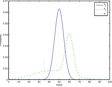
POMDP policy selection dictates that a policy with a maximum expected utility be taken as optimal. Let us concentrate on this notion of expectation. Consider two policiesπ1andπ2applied to the same POMDP,
and distributions of the (accumulated) value under these two policiesD1 andD2 respectively, as shown
in Figure 2. POMDP optimization dictates that the policyπ1should be selected and applied at all times.
However, the variance of the value underπ1is high, which means that if a critical value exists below which
the gain is forbidden to drop (as denoted byαin Figure 2) —π1may not be suitable.
0 10 20 30 40 50 60 70 80 90 100 0
0.01 0.02 0.03 0.04 0.05 0.06 0.07
Value
Probability
[image:5.595.200.395.267.420.2]π2 π1 α
Figure 2: Value distribution under POMDP policies
The expectation problem can be discussed from another point of view, that of system development. POMDP policies can be seen as a solution set for a Sequential Decision Making (SDM) problem. Each pol-icy creates a distribution over system developments (state-action sequences), and one has to choose among different policies based on a comparison of distributions. An SDM problem defines a preference order over system development, in a sense, determining an ideal system development and a measure of divergence be-tween development sequences. The POMDP concept of solution combines policy-induced distribution and SDM-induced preference over the state-action sequences by assigning real values to sequences and optimiz-ing over the value expectation. Returnoptimiz-ing to our previous argument, we see that POMDP-optimal policy can have a very high probability of large deviations from an ideal system development sequence, a property unintended by, and not desired by, the SDM formulation.
3.1.2 Controller Similarity
Although POMDP policies can be history dependent, description length feasibility argues that a policy will have only finite (and rather small) variability in response to different system developments that actually take place. This, together with off-line computation and optimality based on average performance, underscores
Issue POMDPs (see 3.1) DBC (see 3.2)
Action Selector Off-line computed policy On-line action selection Controller Similarity Open-loop (3.1.2) Closed-loop (3.2.1)
User preference interpretation State value oriented (3.1.3) Transition frequency oriented (3.2.2) Optimality concept Expectation oriented (3.1.1) Context dependent, situated (3.2.3)
Complexity PSpace Unknown for DBC
[image:5.595.89.509.667.744.2]POMDP policies’ inability to adapt and change for a specific system development that actually occurs, and which deviates from the expected development under application of the policy.
3.1.3 User Preference Interpretation
POMDP solutions also exhibit a form of user-preference distortion. By formal definition, reward/cost is obtained based on specific transitions exhibited by the system. However, a POMDP’s induced policy is computed with respect to a Value Function, which is a state-oriented, rather than transition-oriented, concept. This may potentially cause distortion of User preferences when expressed by the reward structure.
3.2
Properties of DBC-Induced Policy
Dynamics Based Control (DBC) is a closed-loop control scheme, and action selection is bound to a system development that actually occurs at run-time. DBC is also directly tied to system-transition preference, expressed as the ideal system dynamics.
3.2.1 Controller Similarity
DBC is a situated, context-dependent scheme because it uses an estimation algorithmL that is used to identify the system development that actually takes place at run-time. In fact, DBC (and EMT-based control as a representative of a DBC scheme) takes this to an extreme, in that it viewsLas the “actual” system, and selects actions in a way that leadsLto a required estimate.
It is important to note thatLis not influenced directly; otherwise, its estimate and DBC action-selection make no sense. Rather, L is influenced only through the environment that it estimates. This mode of operation is most similar to a closed-loop differential controller, and is explicitly on-line.
Note, also, that DBC formally is not a learning, tracking, or estimation algorithm by itself, although it has a tracking (estimator) component utilized with its structure.
3.2.2 User Preference Interpretation
The DBC discussion and POMDP discussion above can be unified by taking the point of view of distribu-tions over different system development sequences. Unlike POMDP, the DBC framework attempts a direct comparison between distributions over system development sequences. This is done by considering “induc-tor” stochastic functions, that represent different stochastic behaviors and thus different distributions over system development sequences. DBC assumes that the ideal system development sequence and the measure of deviation from it can be combined into such an “inductor” function,q— the ideal system dynamics. The learning/tracking algorithmLis then used to seek the same form of representation for the actual system development,τ.
3.2.3 Optimality Concept
A DBC policy considersτ andq, that is, the “estimated actual” and the “ideal” distributions over system development sequences, and selects an action based on their direct comparison. The DBC concept of op-timality is based on a threshold probability, and an optimal policy is the one that is capable of keeping deviation from the ideal system dynamics below the threshold with highest probability.
4
EMT-based Control as a DBC
Recently, a control algorithm was introduced called EMT-based Control [9, 10], whose scheme fits perfectly into the DBC framework. Although it presents an approximate greedy solution in the DBC sense, initial experiments using EMT-based control have been encouraging [11]. EMT-based control is based on the Markovian environment definition, as in the case with POMDPs, but its User and Agent Levels are of the DBC type.
• User Level of EMT-based control defines a limited-case, idealized system dynamics independent of
momentary system dynamics estimator — the Extended Markov Tracking (EMT) algorithm. The al-gorithm keeps a system dynamics estimateτt
EM Tthat is capable of explaining recent change in an
aux-iliary Bayesian system state estimator frompt−1topt, and updates it conservatively using
Kullback-Leibler divergence. SinceτEM Tt andpt−1,tare respectively the conditional and marginal probabilities
over the system’s state space, “explanation” simply means thatpt(s0) =P
s
τEM Tt (s
0|
s)pt−1(s), and
the dynamics estimate update is performed by solving a minimization problem:
τt
EM T =H[pt, pt−1, τt
−1
EM T] = arg minτ DKL(τ×pt−1kτ
t−1
EM T×pt−1)
s.t. pt(s0) =P
s
(τ×pt−1)(s0, s)
pt−1(s) =P
s0
(τ×pt−1)(s0, s)
• Agent Level in EMT-based control is sub-optimal with respect to DBC (though remains within the
DBC framework),performing a greedy action selection based on prediction of EMT’s reaction. The prediction is based on the environment model provided by the Environment Design level, so that if we denote byTathe environment’s transition function limited to actiona, andpt−1the auxiliary Bayesian
system state estimator, then the EMT-based control choice is described by
a∗
= arg min
a∈ADKL(H[Ta×pt, pt, τ
t
EM T]kqEM T×pt−1)
Note that this follows the DBC framework precisely; a dynamics estimator (EMT in this case) is manip-ulated via action effects on the environment to produce an estimate close to the idealized system dynamics. Yet naive EMT-based control is suboptimal in the DBC sense, and has several additional limitations that do not exist in the general DBC framework.
4.1
EMT-based Control Limitations
EMT-based control is a sub-optimal (in the DBC sense) representative of the DBC structure. It limits the User by forcing EMT to be its dynamic tracking algorithm, and replaces Agent optimization by greedy action selection. This kind of combination, however, is common for on-line algorithms. Although further development of EMT-based controllers is planned, evidence so far suggests that even the simplest form of the algorithm possesses a great deal of power, and trends that are optimal (in the DBC sense of the word).
There are two further, EMT specific, limitations to EMT-based control that are evident at this point. Both already have partial solutions and are subjects for future research.
The first limitation is the problem of negative preference. In the POMDP framework for example, this is captured simply, through the appearance of values with different signs within the reward structure. For EMT-based control, however, negative preference means that one would like to avoid a certain distribution over system development sequences; EMT-based control, however, concentrates on getting as close as possible to a distribution. Avoidance is thus unnatural in native EMT-based control.
The second limitation comes from the fact that standard environment modeling can create pure sensory
actions — actions that do not change the state of the world, and differ only in the way observations are
received and the quality of observations received. Since the world state does not change, EMT-based control would not be able to differentiate between different sensory actions.
Notice that both of these limitations of EMT-based control are absent from the general DBC framework, since it may have a tracking algorithm capable of considering pure sensory actions and, unlike Kullback-Leibler divergence, a distribution deviation measure that is capable of dealing with negative preference. Furthermore, as was mentioned, EMT-based control itself has a number of possible extensions that promise to be less prone, or not at all prone, to the aforementioned limitations.
5
Conclusions and Future Work
changes of system state and its estimation, DBC attempts to estimate and vary the qualitative features of system modulations. A Dynamics Based Controller can operate either as a direct mixer of available sources of system dynamics, or as a simulator with respect to a given dynamics estimator.
The DBC framework, even limited to well-studied Markovian environments, significantly differs in its approach and the resulting control signal (action policy) from the classical control approach, as represented (for example) by Partially Observable Markov Decision Processes.
Although at this point a complete and exact solution of the DBC framework is not available, a promising beginning in this direction exists — control based on Extended Markov Tracking (EMT) [9, 10]. EMT-based control is computationally efficient, and in fact is polynomial in environment description parameters. Initial experiments using EMT-based control have been encouraging [11].
EMT-based control does have limitations, the main two being negative dynamics preference and pure sensory actions. It seems, however, that extended state representations may resolve these problems, and this direction is currently under investigation.
DBC also requires extensive feasibility and complexity studies, paralleling those done for POMDPs, as well as utilizing its potential for composition of learning algorithms. The latter would be significant for the field of robotics, providing flexible automated techniques for environment model calibration simultaneous with task performance. In this direction it would be interesting to take a closer look at the application of EMT combined with EM, as the latter can use Kullback-Leibler divergence for its operation, thus directly making use of information from an EMT-based controller.
6
Acknowledgment
This work was partially supported by grant #039-7582 from the Israel Science Foundation.
References
[1] Ronald C. Arkin. Behavior-Based Robotics. MIT Press, 1998.
[2] Jeff A. Bilmes. A gentle tutorial of the EM algorithm and its application to parameter estimation for Gaussian mixture and Hidden Markov Models. Technical Report TR-97-021, Department of Electrical Engineering and Computer Science, University of California at Berkeley, 1998.
[3] Chi-Tsong Chen. Linear System Theory and Design. Oxford University Press, 1999.
[4] T. M. Cover and J. A. Thomas. Elements of information theory. Wiley, 1991.
[5] Marie E. desJardins, Edmund H. Durfee, Charles L. Ortiz, and Michael J. Wolverton. A survey of research in distributed, continual planning. AI Magazine, 4:13–22, 1999.
[6] Vijay R. Konda and John N. Tsitsiklis. Actor-Critic algorithms. SIAM Journal on Control and
Opti-mization, 42(4):1143–1166, 2003.
[7] Omid Madani, Steve Hanks, and Anne Condon. On the undecidability of probabilistic planning and related stochastic optimization problems. Artificial Intelligence Journal, 147(1–2):5–34, July 2003.
[8] Radford M. Neal and Geoffrey E. Hinton. A view of the EM algorithm that justifies incremental, sparse, and other variants. In M. I. Jordan, editor, Learning in Graphical Models, pages 355–368. Kluwer Academic Publishers, 1998.
[9] Zinovi Rabinovich and Jeffrey S. Rosenschein. Extended Markov Tracking with an application to control. In The Workshop on Agent Tracking: Modeling Other Agents from Observations, at the Third
International Joint Conference on Autonomous Agents and Multiagent Systems, pages 95–100,
New-York, July 2004.
[11] Zinovi Rabinovich and Jeffrey S. Rosenschein. Robot-control based on Extended Markov Tracking: Initial experiments. In The Eighth Biennial Israeli Symposium on the Foundations of Artificial
Intelli-gence, Haifa, Israel, June 2005.