Optimal harvesting strategy based on rearrangements of functions

(1)

Optimal Harvesting Strategy Based on Rearrangements of

Functions

∗

Behrouz Emamizadeh† _{Amin Farjudian}‡ § _{Yichen Liu}¶

Abstract

We study the problem of optimal harvesting of a marine species in a bounded domain, with the aim of minimizing harm to the species, under the general assumption that the fishing boats have different capacities. This is a generalization of a result of Kurata and Shi, in which the boats were assumed to have the same maximum harvesting capacity. For this generalization, we need a completely different approach. As such, we use the theory of rearrangements of functions. We prove existence of solutions, and obtain an optimality condition which indicates that the more aggressive harvesting must be pushed towards the boundary of the domain. Furthermore, we prove that radial and Steiner symmetries of the domain are preserved by the solutions. We will also devise an algorithm for numerical solution of the problem, and present the results of some numerical experiments.

Keywords:Population biology, Rearrangements of functions, Reaction-diffusion, Optimization, Symmetry.

Mathematics Subject Classification:35K57, 35Q92, 35J25, 65K10, 65K15

1 Introduction

Kurata and Shi [KS08] considered the problem of optimal harvesting of a marine species with the aim of minimizing harm to the species. From an applied marine economy perspective, the main result of their work is a formal argument in support of designation of no-harvesting zones.

To be more precise, consider a species of (say) fish living in a lakeΩwith boundary∂Ω. The species is a source of income for fishermen, and as such, it is imperative to come up with harvesting strategies that, on the one hand, allow the fishermen to make a living, and on the other hand, minimize harm to the species and provide long term sustainability of the source of income.

In mathematical biology, reaction-diffusion equations have provided a standard model for the study of population dynamics of many species. Assuming thatwdenotes the population density, a fairly general form of a reaction-diffusion equation may be expressed as:

∂w/∂t=∇ ·(D∇w)+ f(w,x,t), x∈Ω,t>0, (1)

in which f is regarded as the source function [Mur02, Chap. 11]. For modelling the fish population in a lake, we consider the same set of assumptions as taken by Oruganti, Shi, and Shivaji [OSS02], i. e.:

1. The fish move around via a ‘random walk’ in the boundedhomogeneousenvironmentΩ, which im-plies that Dis constant throughout the domain. Of course, in a more general setting, it could be a function ofw,x, andt.

2. The population dynamics is subject to logistic growth.

With these assumptions, one obtains the following equation:

∂w/∂t= D∆w+aw(1−w/K), x∈Ω,t>0, (2)

where D > 0, and in which a,K > 0 denote the linear reproduction rate and the carrying capacity of the environment, respectively. If the species is subject to harvesting, then a further term should be subtracted from the right hand side of (2) to account for the loss of population due to harvesting. Hence, the modified equation takes the form:

∂w/∂t=D∆w+aw(1−w/K)−h(x,w), x∈Ω,t>0, (3)

in whichh(x,w) denotes the harvesting density per unit time.

As we are interested in qualitative properties of solutions, we would like to make some simplifications in order to turn (3) into a more manageable one. First, we assume that the harvesting density per unit time is directly proportional to the densitywand some harvesting effortE(x) at each point x ∈Ω. Hence, we take

hto be of the form:

h(x,w)=E(x)w.

This is acceptable as, for instance, fishers would cast the same type of net at a pointx∈Ωregardless of the density of population at that point.

Second, to avoid clutter, we would like to take the specific values thataandKtake out of the discussion. To that end, we introduce the change of variablesw(x,t)=K u(y,t) andy= √a xinto (3), which leads to:

(3)

Indeed, for qualitative analysis of the solutions, the parametera appearing in the right hand side has no significance in what shall follow (see, e. g., [CC89]). Hence, we normalize the value ofato 1. Combining the effects of all the simplifications, and by taking the diffusion scaleto beB

√

D, we obtain:

∂u/∂t=2∆u+u−u2−E(y)u, y∈Ω0,t>0.

Regarding boundary conditions, we assume that the surrounding area of the region Ω is completely inhospitable, e. g.,Ωis a lake surrounded by land. This leads to the choice of Dirichlet boundary conditions. We remark here that a more general problem may be studied by considering Robin boundary conditions, but as, on the one hand, our focus in this article is not the effects of the boundary conditions, and on the other hand, with Dirichlet boundary conditions we have richer mathematical results at our disposal, we focus on the case of Dirichlet boundary conditions.

Putting together all the normalizations, simplifications, and considerations alluded to thus far leads to the dynamics of the fish population being modeled by the following reaction-diffusion equation with logistic growth:

            

∂u/∂t=2∆u+u−u2−E(x)u, x∈Ω,t>0,

u(x,t)=0, x∈∂Ω,t>0,

u(x,0)=u0(x), x∈Ω,

(4)

in which:

• Ω⊆_RN_{is a smooth domain, with}_N_≥_1;

• uis the population density;

• u0≥0 is an initial population density;

• is the diffusion scale;

• E(x)≥0 is the harvesting effort, and as a consequence,E(x)uis the harvesting density per unit time;

• All the variables are dimensionless.

Thebiological energy functionassociated with system (4) is given as follows:

E(u,E)B

2

Z

Ω| ∇u|

2_d_x

| {z }

kinetic energy

−1 2

Z

Ωu

2_d_x₊ 1

3

Z

Ωu

3_d_x₊ 1

2

Z

ΩE(x)u

2_d_x

| {z }

potential energy

, (5)

for u ∈ H₀1(Ω). As time passes, this quantity decreases for u(·,t). To see this, observe that using the Divergence theorem, and keeping in mind that∂u/∂tvanishes on∂Ω, one finds:

dE(u(·,t))

dt =

Z

Ω h

−2∆u−u+u2+E(x)ui∂u

∂tdx

= −

Z

Ω ∂u

∂t

!2

dx≤0,

fort∈(0,∞). This behavior ofE(u(·,t)), coupled with the fact thatE(u(x,t),E)≥ −C, for some positive constantC,1guarantee that there exists a functionu∞ ∈H₀1(Ω) such that:

lim

t→∞ku(x,t)−u∞(x)kH10(Ω) =0.

(4)

The functionu∞satisfies the following steady state equation:

      

2_∆_u₊_u₋_u2₋_E₍_x₎_u₌₀_, _x_∈_Ω_,

u(x)=0, x∈∂Ω. (6)

Of particular interest is the long term survival of the species which, according to the current formalism, is determined by the steady state solutionuof (6). As the effort functionE(x) is the only parameter under our control, we denote the solution of (6) byuE, to stress its dependence on the harvesting strategy. Indeed,

it has been shown (see, e. g., [CC89]) that when the diffusion scale is small enough, and the harvesting effort is not too aggressive—i. e., when{x∈Ω | E(x)<1}has positive measure—the population survives, in that equation (6) has a unique positive solutionuE, which satisfies:∀x∈Ω: 0<uE(x)≤1.

Nonetheless, the survival of the species is not the same as its well-being. We have already discussed how the solutionu(x,t) of the parabolic equation (4) descends (in energy terms) towards a minimum energy steady state. This hints at the biological system’s preference towards lower energy. By fixing, and noting the dependence ofuEonE—which is the parameter under our control—we define:

Φ(E)B

2

Z

Ω| ∇uE|

2_d_x ₋ 1

2

Z

Ωu

2

Edx+

1 3

Z

Ωu

3

Edx+

1 2

Z

ΩE(x)u

2

Edx. (7)

By incorporating the differential equation in (6) into the definition ofΦin (7), it can be shown that:

Φ(E)=−1 6

Z

Ωu

3

Edx.

To maximize the well-being of the species, our aim should be to devise a harvesting strategy E(x) which minimizesΦ(E) amongst all the admissible choices forE(x). This is equivalent to maximizingR_Ωu3_Edx, a quantity which, at an intuitive level, may be construed as atotal population distributionin the habitat. This also reinforces the idea of minimizingΦin order to maximize the well-being of the species. To that end, Kurata and Shi [KS08] consider the following assumptions onE(x):

1. Among all the admissible choices forE(x), the total effort is constant:

Z

ΩE(x) dx=β· |Ω|, (8)

in whichβ >0 is the average effort, and|Ω|denotes the Lebesgue measure ofΩ.

2. The effort functionE(x) is non-negative and bounded, i. e., for a maximum allowable harvesting effort

M≥β:

∀x∈Ω: 0≤E(x)≤ M. (9)

It is well known that the set

E0 _B

(

E∈L∞(D) 0≤ E(x)≤ M,

Z

ΩE(x) dx=β· |Ω|

) ,

which is exactly the admissible set of effort functions satisfying (8) and (9), is theσ(L2,L2)-closure of the set

E_B

MχA Ais a Lebesgue-measurable subset ofΩand|A|= β

M|Ω|

, (10)

in whichχAis the characteristic function of the setA, see, e. g., [LE16, Lemma 4.1]. Here,σ(L2,L2) denotes

the weak topology onL2(Ω) induced byL2(Ω).

(5)

solution is of a ‘bang-bang’ type, meaning that there must be a no-harvesting zone (of maximum measure possible) set aside over which no harvesting is allowed, and outside of which harvesting is carried out with maximum allowable effort. The authors go on to prove other interesting results regarding the location and geometry of the no-harvesting zone, e. g., that it preserves the Steiner symmetry of the domainΩ, and that symmetry breaking can happen over non-convex domains such as the dumbbell shaped domain and annulus. It is also argued that the no-harvesting zone must in general be away from the boundary ofΩand closer to the center of the domain.

1.1 Our alternative approach through rearrangements of functions

In this paper, we obtain a generalization of the result of Kurata and Shi [KS08] through the theory of rearrangements of functions as developed by G. R. Burton [Bur87; Bur89b; Bur89a]. Note that the setEin (10) is indeed arearrangement class(see Definition 3 on the next page). Thus, here we attack the problem from another angle. We first consider the optimization problem over a given rearrangement class, and then prove its solvability by relaxing the admissible set to its weak closure. In contrast to the result of [KS08] where the rearrangement class had to be generated by a characteristic function, here we can consider the

general multivalued generators.

The interpretation of the multivalued setting is as follows: imagine a fishing fleet consisting of boats of various capacities, and assume that, to make the deployment of each boat cost-effective, each boat is required to harvest to its maximum capacity. The problem is to find the best spatial strategy regarding the location of the boats.

Note that, if all the boats have the same capacity, the problem reduces to that considered in [KS08]. Here we solve the general multivalued problem using the theory of rearrangements of functions. Furthermore, we obtain an optimality condition, which in particular provides a generalization of the result of [KS08] regarding the location of boats. Specifically, it will be shown that the larger boats must be deployed closer to the boundary of the habitat.

Finally, we will develop an algorithm for numerical solution of the multivalued problem and present the results of some numerical experimentations. These results verify some of the theoretical conclusions of [KS08] and the current paper.

1.2 Structure of the paper

The rest of the paper is organized as follows:

• Section 2 contains the preliminaries on rearrangement theory and some basic properties of the steady state equation (6).

• Existence of solutions will be proven in Section 3.

• We prove preservation of Steiner and radial symmetries in Section 4.

• In Section 5, we present a numerical algorithm for finding minimizers, together with a number of figures from our experiments that verify the theory.

• To avoid a large gap in the flow of the content, we have included the lengthy proof of Lemma 13— from Section 3—in Section 6. This is an essential lemma which deals with the fundamental properties of the energy functionalΦ.

(6)

2 Preliminaries

The material in this section includes some basic results from the theory of rearrangements of functions, and some background on the steady state equation (6), which we will need later on.

2.1 Rearrangements of functions

For a Lebesgue measurable functionh:Ω→[0,∞) andα≥0, we let:

λh(α)B| {x∈Ω|h(x)≥α} |.

Definition 1. Let g₀ : Ω1 → [0,∞) and g : Ω2 → [0,∞) be Lebesgue measurable. We say that g is a rearrangement of g0if and only if∀α≥0 :λg0(α)=λg(α).

Definition 2. For a Lebesgue measurable g : Ω → [0,∞), the essentially unique decreasing rearrange-ment g∆of g is defined on(0,|Ω|)by g∆(s) B max{α∈R | λg(α)≥s}. The essentially unique increasing

rearrangement g_∆of g is defined by g_∆(s)Bg∆(|Ω| −s).

Definition 3. The rearrangement classR(g0)generated by g0is defined as follows:

R(g0)B{g:Ω→[0,∞) g is a rearrangement of g0}.

When the generator is clear from the context, we may simply writeR.

Definition 4. For a function f : Ω → _R, we say that the graph of f has no significant flat zones onΩif

∀c∈_R:| {x∈Ω f(x)=c} |=0.

Lemma 5. Let g0∈L∞(Ω)+, where L∞(Ω)+denotes the positive cone generated by non-negative functions in L∞(Ω). LetRbe the weak closure ofR_BR(g₀)in L2(Ω). Then,R ⊆ L∞(Ω), and∀g∈ R:kgk_∞≤ kg₀k_∞.

Proof. Letg∈ R, and assume thatDB{x∈Ω|g(x)>kg0k∞}has a positive Lebesgue measure. Asg∈ R,

there exists{gn} ⊆ Rsuch thatgn *ginL2(Ω). Then, we have:

Z

D

gndx= Z

ΩgnχDdx→

Z

ΩgχDdx=

Z

D

gdx. (11)

As eachgnis in the rearrangement class ofg0, we have

R

Dgndx ≤ kg0k∞|D|. On the other hand, from the

definition ofD, in conjunction with (11), we deduce:

kg₀k_∞|D|<

Z

D

gdx= lim

n→∞ Z

D

gndx≤ kg0k∞|D|,

which is a contradiction. As a result, the measure ofDis zero, andkgk_∞ ≤ kg0k∞.

Lemma 6. Assume that{gn}n∈Nis a sequence of non-negative functions in L

∞_(Ω)_{, g}_∈ _L2_(Ω)_{, and g}

n *g

in L2(Ω). Then, g is non-negative a.e. inΩ.

Proof. By Mazur’s Lemma, there exists a sequence{vn} in the convex hull of the set{gn | n∈N}, such

thatvn → g inL2(Ω). Therefore, vn → gin measure. Whence, there exists a subsequence of{vn}which

converges togalmost everywhere inΩ. This completes the proof.

Lemma 7. Let g0 ∈ L2(Ω)+, and let R B R(g0). Suppose Ψ : R → R is convex, weakly sequentially

continuous, and satisfies the following:

lim

t→0+

Ψ(u+t(v−u))−Ψ(u)

t =

Z

ΩG(u)(v−u) dx, ∀v,u∈ R, (12)

(7)

(i) Ψattains a maximum value relative toR.

(ii) Letu be a maximizer forˆ Ψrelative toR, and supposeΨis locally strictly convex atu, i. e.ˆ

∃ >0 : Ψ is strictly convex on R ∩B( ˆu, ),

Then,uˆ =η◦G( ˆu)a.e. inΩ, for some non-decreasing functionη.

Proof.

(i) We begin by considering the following maximization problem:

sup

u∈R

Ψ(u). (13)

Since Ψis weakly continuous, and Ris weakly compact, (13) is solvable. Let ¯u ∈ R be a solution. By applying the formula (12), we infer that ¯u maximizes the continuous linear functional L(h) :=

R

ΩG( ¯u)h dxrelative toh∈ R. It is known that the functionalLhas a maximizer ˜urelative toR[Bur87,

Theorem 4]. Since L is weakly continuous, it follows that ˜u maximizes L relative to R as well. Whence, in particular,L( ¯u)≤ L( ˜u).By using the convexity ofΨand the formula (12), we have:

Ψ( ˜u)−Ψ( ¯u)≥ lim

t→0+

Ψ( ¯u+t( ˜u−u¯))−Ψ( ¯u)

t =

Z

ΩG( ¯u)( ˜u−u¯) dx=L( ˜u−u¯)≥0.

Thus,Ψ( ˜u)= Ψ( ¯u), and ˜u∈ Ris a solution of (13), as desired.

(ii) Let us fix a maximizer ˆusatisfying the local strict convexity. For anyv ∈ R, there existst> 0 small enough such that:

0≥Ψ(v)−Ψ( û)> Ψ( û+t(v−uˆ))−Ψ( û)

t ≥

Z

ΩG( ˆu)(v

−uˆ) dx,

where the second inequality follows from local strict convexity of Ψat ˆu, and the third inequality is derived from the convexity ofΨ. Thus, ˆuis the unique maximizer of the continuous linear functional L₁(v) B

R

ΩG( û)vdxrelative tov ∈ R. By applying Theorem 5 in [Bur87], we infer û=η◦G( û) a.e.

inΩ, for some non-decreasing functionη, as desired.

2.2 Steady state equation (6)

We need the following result regarding existence and uniqueness of solutions of the boundary value problem (BVP) (6):

Proposition 8. Assume that| {x∈Ω|E(x)<1} |>0. Then, there exists an₁=₁(Ω,E)>0such that:

• When ≥₁, the BVP (6) has only the trivial solution uE =0.

• When0< < 1, the BVP (6) has a unique positive solution, which is positive throughout the (interior

of the) domain, and bounded above by1, i. e.:

∀x∈Ω: 0<uE(x)≤1.

Furthermore, this solution is globally asymptotically stable, in the sense that, for any u0∈L2(Ω)with u0(x)≥0for all x∈Ω, the solution u(x,t)of the parabolic equation (4) satisfies:

lim

(8)

Proof. See [CC89, Sect. 2].

Remark 9. There is indeed an explicit description of the value₁of Proposition 8. Consider the following eigenvalue problem:

      

−∆z=λ(1−E(x))z, x∈Ω,

z=0, x∈∂Ω, (14)

and letλ+₁ be the smallest positive eigenvalue of (14). Then1 = √1_λ₊

1

. For further details, see [CC89,

Sect. 2].

3 Existence of solutions

Let us first go through the formal statement of the problem. We take a non-negative functionE0 ∈L∞(Ω) as

the generator of the rearrangement classR(E0), whereE0satisfies:

1 |Ω|

Z

ΩE0(x) dx<1. (15)

Each element of this rearrangement class represents a harvesting strategy, and for eachE∈ R(E₀) andx∈Ω, the valueE(x) corresponds to the harvesting capacity of the boat located atx. The special case whereE0

is a characteristic function corresponds to the one considered in [KS08], where all the boats have the same capacity.

Since 1 depends onE when Ωis fixed, we need to maximize the 1 among the rearrangement class

R(E0), i. e.:

2(E0) := sup

E∈R(E0)

1(Ω,E). (16)

Proposition 10. Let E0be a non-negative function in L∞(Ω)which satisfies (15), and letRBR(E0). Then,

the maximization problem (16) is solvable. Furthermore, for any maximizerE, there exists a non-decreasing˜

functionϕsuch thatE˜ =ϕ◦uE˜.

Proof. By Remark 9, the maximization problem (16) is equivalent to the following minimization problem:

1

2(E0)2

= inf

E∈R(E0)

λ+₁(E). (17)

By applying Theorem 1 (i) in [CCP13], we have the desired results.

Remark 11. We know that ₁(Ω,·) is continuous on R [CCP13, Prop. 1 (i)]. For < ₂, there exists E1∈ R(E0)such that < 1(Ω,E1), while it is possible to have ≥1(Ω,E2)for some other E2 ∈ R(E0).

Now, let us fix a positive < 2(E0). We are interested in minimizing harm to the species, which

corresponds to minimization of the functional:

Φ(E)B

2

Z

Ω| ∇uE|

2_d_x ₋ 1

2

Z

Ωu

2

Edx+

1 3

Z

Ωu

3

Edx+

1 2

Z

ΩE(x)u

2

Edx=−

1 6

Z

Ωu

3

Edx (18)

over the setR(E0) of all the admissible strategies. We denote this problem by the usual notation:

inf

E∈R(E0)

Φ(E). (19)

(9)

Lemma 12. If—by a slight abuse of notation—we define:

Φ(v,E)B

2

Z

Ω| ∇v|

2_d_x ₋1

2

Z

Ωv

2_d_x₊1

3

Z

Ωv

3_d_x₊1

2

Z

ΩE(x)v

2_d_x_, ₍₂₀₎

then we have:

Φ(E)= inf

v∈H1 0(Ω)+

Φ(v,E). (21)

Indeed, for each fixed E, the solution uE of the BVP (6) is the unique minimizer ofΦ(v,E)with respect to

v∈H₀1(Ω)+.

Proof. SinceE(x)≥0, for everyv∈H1₀(Ω)+, we have

Φ(v,E)≥

2

2 kvk

2

H1₀(Ω)−

1 2

Z

Ωv

2_d_x₊1

3

Z

Ωv

3_d_x₌ 2

2 kvk

2

H₀1(Ω)+

1 6

Z

Ωv

2₍₂_v₋_{3) d}_x

≥

2

2 kvk

2

H1 0(Ω)+

1 6

Z

{v<3 2}

v2(2v−3) dx≥

2

2 kvk

2

H1 0(Ω)

− 9

8|Ω|. (22)

So,Φ(·,E) is coercive and bounded below onH₀1(Ω)+. By applying the direct method of calculus of vari-ations, we infer the existence of a minimizerv for (21). We intend to show thatv = uE, in the sense of

Proposition 8. To that end, we apply the classical techniques of variational inequalities, (see, e. g., [Eva10, Sect. 8.4.2]). It follows that:

      

v≥0, −2∆v≥(1−E(x))v−v2, inΩ,

−2∆v=(1−E(x))v−v2, onΩ∩ {v>0}. (23)

However, in the region {x∈Ω | v(x)=0}, the differential equation in the second line of (23) is trivially satisfied. This implies that the minimizer satisfiesv = 0 orv = uE. If ≥ (Ω,E), we must havev = 0.

On the other hand, if < (Ω,E), we infer thatv = uE is the unique positive solution, since Φ(uE,E) =

−1₆R_Ωu3_Edx<0.

Lemma 13. Let E0be a non-negative function in L∞(Ω)which satisfies (15), and letRBR(E0). Suppose that0< < 2(E0). The functionalΦ:R →Rsatisfies the following properties:

(i) Φis weakly sequentially continuous w. r. t. the L2topology.

(ii) Φis concave. Moreover, for any E ∈ Rwith uE >0,Φis locally strictly concave at E, i. e.:

∃ >0 : Φ is strictly concave on R ∩B(E, ).

(iii) For any given E and F inR, by assigning vBF−E, we get:

lim

t→0+

Φ(E+tv)−Φ(E)

t = 1 2 Z Ωvu 2

Edx. (24)

Proof. See Section 6.

Based on the properties of the energy functional as stated in Lemma 13, we can apply the theory of Burton [Bur87] to obtain the following existence result:

Theorem 1. Let E0be a non-negative function in L∞(Ω)which satisfies (15), and let0< < 2(E0). Then,

the minimization problem (19) is solvable. Furthermore, for any minimizer E∗, there exists a non-increasing

functionφˇ such that:

(10)

Proof. DefineΨ(E) B −Φ(E). By Lemma 13, the functionalΨ is weakly sequentially continuous w. r. t.

theL2topology, convex, and satisfies the formula (12) withG(E)=−1₂u2_E. Thus, we can apply Lemma 7 to deduce that the maximization problem:

sup

E∈R(E0)

Ψ(E) (26)

is solvable.

Let us fix a maximizer E∗ ∈ R(E₀), and note that we must have uE∗ > 0 by Remark 11. It follows from Lemma 13 (ii) thatΨis locally strictly convex atE∗. By Lemma 7 (ii), we haveE∗ = φˆ ◦(−1₂u2_E∗), for some non-decreasing function ˆφ. This implies thatE∗ = φˇ◦uE∗, in which ˇφ : [0,∞) → _R, defined by

ˇ

φ(t)Bφˆ(−t2/2), is non-increasing.

It should be obvious that any solution of the maximization problem (26) is a solution of our main

minimization problem (19), and vice versa. Hence, the proof is complete.

4 Symmetry results

In this section, we investigate preservation of Steiner and radial symmetries by the minimizer, whenΩhas the respective symmetries.

Theorem 2. Suppose that | {x∈Ω|E0(x)=kE0k∞} | > 0. If Ω is Steiner symmetric with respect to a

hyperplane P, then E∗is increasingly Steiner symmetric with respect to the hyperplane P.

Proof. The proof is similar to Theorem 2.5 in [KS08]. Without loss of generality, we assume thatΩ is

Steiner symmetric with respect to the hyperplanex₁=0. LetE∗be a minimizer of the optimization problem withE∗=φ˘◦uE∗ for a non-increasing ˘φas shown in Theorem 1. Then, we have:

−2∆uE∗ =(1− kE₀k_∞−u_E∗)u_E∗ +(kE₀k_∞−φ˘◦u_E∗)u_E∗.

Let us set f1(u)B(1− kE0k∞−u)uand f2(u)B(kE0k∞−φ˘◦u)u. By applying Theorem 3.6 in [Fra00], we

conclude thatuE∗ is decreasingly Steiner symmetric with respect to the hyperplane x₁ = 0. Recalling that

E∗=φ˘ ◦uE∗, we infer thatE∗is increasingly Steiner symmetric with respect to the hyperplanex₁=0.

The following is a direct consequence:

Corollary 14. Suppose that| {x∈Ω|E0(x)=kE0k∞} | > 0. IfΩis a ball centered at the origin, then E∗

is increasingly Schwarz symmetric with respect to the origin. Moreover, E∗is the unique minimizer of the

optimization problem (19).

Remark 15. The assumption| {x∈Ω|E0(x)=kE0k∞} |> 0is a reasonable one, as in practice we expect

the maximal harvesting to be taken over a region rather than at a point.

5 Numerical algorithm

The gradient formula (24) of Lemma 13, together with the optimality condition 25 of Theorem 1, give us the necessary machinery for devising a numerical algorithm for solving the minimization problem (19), which is only practical when the generator E0 is a characteristic function. For an example of such an algorithm,

see [EFZR16].

Fortunately, for the current problem we can devise an algorithm based on the approach of Eydeland and Turkington [ET88], which was also applied to a rearrangement problem by Elcrat and Nicolio [EN95]. The pseudocode in Fig. 1 is a simplified account of the main iteration in our algorithm.

Proposition 16. The iteration of Fig. 1 on the following page generates a minimizing sequence, i. e., at every iteration j we have:

(11)

Figure 1Iteration for generating a minimizing sequence. Input:A generatorE0, and an >0.

Output:An approximation of a local minimum.

1. Start withE0;

2. Set jB0;

3. Repeat

4. Ej+1Barg minE∈R(E0)

R

ΩEujdx, whereujBuEj;

5. jB j+1;

6. Until kEj+1−Ejk∞

kE0k∞ < .

Proof. This is straightforward, as we have:

Φ(Ej)+

1 2

Z

Ω(Ej+1−Ej)u

2

jdx = Φ(uj,Ej+1)

(by Lemma 12) ≥ Φ(uj+1,Ej+1)

= Φ(Ej+1). (28)

Note that by line 4 of the iteration, we have chosen Ej+1 to minimize the functional L1(h) B R_Ωhujdx

relative to the rearrangement class R(E₀). But as uj is non-negative, then Ej+1 also minimizes L2(h) B R

Ωhu2jdx. This implies that:

1 2

Z

Ω(Ej+1−Ej)u

2

jdx≤0,

which, together with (28), prove inequality (27).

5.1 Implementation

We have implemented an algorithm for solving (19) in dimensionN=2, using the iteration of Fig. 1, which provides the basic machinery for generating a minimizing sequence. Here, we discuss a couple of issues regarding concrete implementation of the algorithm.

5.1.1 Discretization and calculation ofEj+1

The only non-trivial step of the iteration is the calculation ofEj+1in Line 4. Suppose that we have a mesh

D={Di |0≤i≤P−1}(for someP∈N) over the domainΩ⊆R2, such thatΩ =∪D. The corresponding discretization of the generator provides a list ofPvalues, which we sort inascendingorder to obtain:

E₀(0)≤E(1)₀ ≤. . .≤ E₀(P−1).

These are the various values that the (discretized) generator takes over (say, the centroid of) each finite elementDi.

At each iteration j, we sort the values ofujover the (say, centroids of the) finite elements, indescending

order, to obtain:

uj(Dσ(0))≥uj(Dσ(1))≥. . .≥uj(Dσ(P−1)),

in whichσ :{0,1, . . . ,P−1} → {0,1, . . . ,P−1}is a permutation. To obtainEj+1, it suffices to assign the

valueE(₀k)to the finite elementDσ(k), fork∈ {0,1, . . . ,P−1}.

Thus, assuming thatujhas already been obtained, the calculation ofEj+1requires a simple sorting ofP

(12)

Remark 17. Care must be taken as the current procedure relies on uj having no significant flat zones.

Indeed, by assuming:

∀c∈[0,1) :| {x∈Ω| E(x)=c} |=0,

it can be shown that uE does not have any significant flat zones. We do not have a proof for the general case,

but in our numerical simulations, none of the uj’s have any flat zones, so we can apply the above procedure.

5.1.2 Local optima and saddle points

We have neither proven nor disproven the existence of non-global local optima or saddle points. Nonethe-less, our numerical experiments strongly indicate the existence of local optima, from which the algorithm cannot escape except through the use of randomization. The local optima show themselves more clearly over the dumbbell shaped domain, in the presence of a very small no-harvesting zone (or zones with very low harvesting effort).

To escape local optima (and potential saddle points), we have enhances the algorithm with randomization through Simulated Annealing. Of course, with randomized algorithms the best one may get is a near-optimal solution, and due to the huge size of the search space, a brute force search is impractical. For more details, please see [EFZR16].

5.2 Experiments and figures

We present the results of some of our numerical experiments. All of the figures have been produced in MATLABR_{. The computations in each case have taken less than 30 seconds on a personal laptop.}

5.2.1 Radial domain

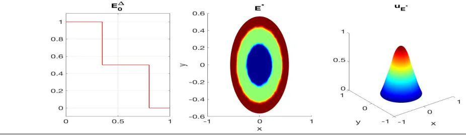
We have considered a disc-shaped lake of area 1. We want to cover 35% of the domain with larger boats, 45% with medium-sized boats, and leave the remaining 20% as the no-harvesting zone. Figure 2 below shows the result of running our algorithm on this domain.

[image:12.612.76.539.553.688.2]

Note that the generator of the rearrangement class is 3-valued. The optimal strategy, as shown in the middle of the figure, suggests that the smaller boats should be positioned closer to the no-harvesting zone, which is in the middle. The larger boats harvest around the boundary. Of course, this is intuitively expected. Note also that radial symmetry is preserved.

Figure 2From left to right: the decreasing rearrangementE₀∆of the 3-valued generatorE0, the best

(13)

5.2.2 Curvy generator

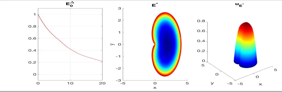
To show that our algorithm works for general multi-valued generators, we have considered a generator with no flat zones at all, over a cardioid of area 20. The result is shown in Fig. 3 below. Starting from a random initial guess E0, the algorithm reaches a stable result in about 60 iterations, under 20 seconds, and with

relative error less than 10−2.8. Here, the relative error at each iteration jis calculated by:

relative error at iterationj= kEj+1−Ejk∞

kE0k∞

=kEj+1−Ejk_∞,

askE0k∞ = 1. A further 100 iterations takes the relative error to just below 10−3, but makes no noticeable

[image:13.612.75.540.242.394.2]

dent in the optimal energy.

Figure 3 Multivalued generator on the cardioid: Again note that the harvesting should be less aggressive towards the center.

5.2.3 Symmetry breaking

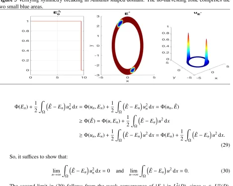
Kurata and Shi [KS08] prove that symmetry breaking can occur for the 2-valued case in dumbbell-shaped and annulus-shaped domains, when the no-harvesting zone is quite small.

In the case of the dumbbell-shaped domain (Fig. 4 on the next page) the two patches must be relatively large, and the channel between them should be relatively narrow. We have considered a domain of area 1, with the no-harvesting zone taking up 8% of the area.

In the case of the annulus, the radius of the two inner and outer circles should be relatively large, and the strip should be quite narrow (Fig. 5 on the following page). Here we have taken the domain to have area 10, and the no-harvesting zone to take up 5% of the total area of the lake.

In both cases, our experiments produce symmetry breaking, as predicted by the theory. Nonetheless, in the case of the dumbbell-shaped domain, Steiner symmetry is preserved, as proven by Kurata and Shi [KS08], and also generalized in Theorem 2 of the current document.

6 Proof of Lemma 13

(i) We follow the approach taken in proving Lemma 3.3 (i) in [EL15]. Consider a sequence{En|n∈N} ⊆ Rand a function ˆE ∈ R, such thatEn *Eˆ inL2(Ω). For simplicity, let us setun BuEn andu BuEˆ.

(14)

[image:14.612.75.539.80.240.2] [image:14.612.77.546.252.626.2]

Figure 4Verifying symmetry breaking in the Dumbbell shaped domain: Note that the no-harvesting zone is the blue zone in the right patch.

Figure 5Verifying symmetry breaking in Annulus shaped domain: The no-harvesting zone comprises the two small blue areas.

Φ(En)+

1 2

Z

Ω

ˆ

E−En

u2_ndx= Φ(un,En)+

1 2

Z

Ω

ˆ

E−En

u2_ndx= Φ(un,Eˆ)

≥Φ( ˆE)= Φ(u,En)+

1 2

Z

Ω

ˆ

E−En

u2dx

≥Φ(un,En)+

1 2

Z

Ω

ˆ

E−En

u2dx= Φ(En)+

1 2

Z

Ω

ˆ

E−En

u2dx.

(29)

So, it suffices to show that:

lim

n→∞ Z

Ω

ˆ

E−En

u2_ndx=0 and lim

n→∞ Z

Ω

ˆ

E−En

u2dx=0. (30)

The second limit in (30) follows from the weak convergence of {En} in L2(D), since u ∈ L∞(D).

However, the verification of the first limit in (30) requires more work. To this end, let us recall that:

      

2_∆_u

n+un−u2n−En(x)un=0, x∈Ω,

un(x)=0, x∈∂Ω.

(15)

By multiplying both sides of (31) byun, and using the divergence theorem, we obtain:

2

Z

Ω| ∇un|

2_d_x ₌

Z

Ω

u2_n−u3_n−Enu2n

dx

(asun≥0, andEn≥0) ≤ Z

Ωu

2

ndx

(by Proposition 8) ≤ |Ω|.

Hence,{un}is a bounded sequence inH₀1(Ω). This, in turn, implies the existence of a subsequence of {un}—still denoted{un}—and ˜u∈H₀1(Ω), such thatun *u˜ inH1₀(Ω), andun →u˜ inL2(Ω). Recalling

that 0≤un≤1, by extracting a further subsequence if necessary, it follows from Lebesgue dominated

convergence theorem thatu2_n →u˜2inL2(Ω). Next, we write:

Z

D

ˆ

E−En

u2_ndx=

Z

D

ˆ

E−En

(u2_n−u˜2) dx+

Z

D

ˆ

E−En

˜

u2dx. (32)

Obviously, the right hand side of (32) tends to zero asngoes to infinity. The proof of item (i) is com-plete.

Before proving the last two properties, we claim that the operatorG:R →L2(Ω) defined byG(E)Bu2_E

is continuous onR, and the set B _B nE ∈ R:G(E)>0ois open inR. We know from Proposition 8 that

for everyE ∈ R,G(E) is either (strictly) positive or zero onΩ. Recalling (18), we infer thatΦ(E) = 0 if

uE =0, andΦ(E)<0 ifuE >0. The openness ofBinRfollows by using the continuity ofΦ. To prove the

continuity ofG, it suffices to show that ˜u=uEˆ. By (31) we have:

∀φ∈C₀∞(Ω) :2

Z

Ω∇un· ∇φdx+

Z

Ω

−unφ+u2nφ+Enunφ

dx=0. (33)

Sinceun*u˜inH1₀(Ω),un →u˜strongly inL2(Ω), andEn*Eˆ inL2(Ω), from (33) we obtain:

∀φ∈C∞₀(Ω) :2

Z

Ω∇u˜· ∇φdx+

Z

Ω

−uˆφ+u˜2φ+Eˆu˜φ dx=0.

Ifu_E_ˆ =0, then it follows from Proposition 8 that ˜u=u_E_ˆ. On the other hand, ifu_E_ˆ >0, we need to show that ˜

u,0. Let us pass to the limit in the following equation:

Φ(En)= 2

2

Z

Ω| ∇un|

2_d_x ₋ 1

2

Z

Ωu

2

ndx+

1 3

Z

Ωu

3

ndx+

1 2

Z

ΩEnu

2

ndx,

which leads to:

0>Φ( ˆE)=lim inf

n→∞ Φ(En)≥ 2

2

Z

Ω| ∇u˜|

2_d_x ₋ 1

2

Z

Ωu˜

2_d_x₊ 1

3

Z

Ωu˜

3_d_x₊ 1

2

Z

Ω

ˆ

Eu˜2dx.

This shows that ˜u,0, as desired.

(ii) Let us first prove that Φ is concave. Take E1,E2 ∈ R, t ∈ (0,1), andEt B tE1+ (1− t)E2. For v∈H1₀(D)+, we have:

Φ(v,Et)=tΦ(v,E1)+(1−t)Φ(v,E2), (34)

in which the bivariate variant Φ(., .) is as in (20). By taking the infimum of both sides of (34) with respect tov∈H₀1(D)+, we obtain:

(16)

which proves the concavity of Φ. We prove the second assertion by contradiction. To that end, by recalling the openness ofB, assume that for someE1∈B\ {E}andt∈(0,1), we have:

Φ(Et)=tΦ(E)+(1−t)Φ(E1). (35)

From (35), and after some straightforward calculations using (21), we obtain:

Φ(uE,E)= Φ(uEt,E) and Φ(uE1,E1)= Φ(uEt,E1).

Once again, by using the minimality of uE anduE1 (Lemma 12), we obtain uE = uEt = uE1. Thus,

substituting in the main BVP (6), we have:

      

2_∆_u

E+uE −u2_E−E(x)uE =0, x∈Ω, 2_∆_u

E1 +uE1 −u2_E1−E1(x)uE1 =0, x∈Ω.

This implies that (E− E1)uE = 0, almost everywhere in Ω. As uE is positive, then we must have

E=E₁, almost everywhere inΩ, which is a contradiction.

(iii) To derive formula (24), we first derive the following equation similar to (29):

∀E1,E2∈ R:

1 2

Z

Ω(E2

−E1)u2E2dx≤Φ(E2)−Φ(E1)≤

1 2

Z

Ω(E2

−E1)u2E1dx. (36)

Now, by settingE1BEandE2 BE+tv=E+t(F−E), from (36) we obtain:

1 2

Z

Ωtv u

2

E+tvdx≤Φ(E+tv)−Φ(E)≤

1 2

Z

Ωtv u

2

Edx,

which implies that: 1 2

Z

Ωv u

2

E+tvdx≤

Φ(E+tv)−Φ(E)

t ≤

1 2

Z

Ωv u

2

Edx, (37)

ast>0. On the other hand, by applying the continuity ofGwe know that limt→0+u2E+tv=u

2

EinL

2₍_Ω_),

which, combined with (37), implies that:

lim

t→0+

Φ(E+tv)−Φ(E)

t = 1 2 Z Ωvu 2

Edx,

as desired.

7 Concluding remarks

The theory behind optimization of convex functionals over rearrangement classes, as used in this paper, was originally laid out by Burton [Bur87] to study vortex rings, i. e., in the context of fluid dynamics. The abstract formulation of rearrangement optimization problems, however, suggests a greater potential for applications. In essence, one has a set of resources which should be deployed to solve a given problem, and the main task is to find the optimal arrangement/permutation of resources.

(17)

References

[Bur87] Burton, G. R. “Rearrangements of functions, maximization of convex functionals, and vortex rings”. In:Math. Ann.276.2 (1987), pp. 225–253.

[Bur89a] Burton, G. R. “Variational problems on classes of rearrangements and multiple configurations for steady vortices”. In:Ann. Inst. H. Poincar´e Anal. Non Lin´eaire6.4 (1989), pp. 295–319.

[Bur89b] Burton, G. “Rearrangements of functions, saddle points and uncountable families of steady configurations for a vortex”. In:Acta Mathematica163.1 (1989), pp. 291–309.

[CC89] Cantrell, R. S. and Cosner, C. “Diffusive logistic equations with indefinite weights: population models in disrupted environments”. In:Proceedings of the Royal Society of Edinburgh: Section

A Mathematics112.3-4 (1989), pp. 293–318.doi:10.1017/S030821050001876X.

[CCP13] Cosner, C., Cuccu, F., and Porru, G. “Optimization of the first eigenvalue of equations with indefinite weights”. In:Adv. Nonlinear Stud.13.1 (2013), pp. 79–95.

[EFL18] Emamizadeh, B., Farjudian, A., and Liu, Y. “Optimal Harvesting Strategy Based on Rearrange-ments of Functions”. In:Applied Mathematics and Computation320 (2018), pp. 677–690.doi: 10.1016/j.amc.2017.10.006.

[EFZR16] Emamizadeh, B., Farjudian, A., and Zivari-Rezapour, M. “Optimization Related to Some Non-local Problems of KirchhoffType”. In: Canad. J. Math. 68.3 (2016), pp. 521–540.doi: 10 . 4153/CJM-2015-040-9.

[EH09] Emamizadeh, B. and Hanai, M. A. “Rearrangements in real estate investments”. In:Numerical

Functional Analysis and Optimization30.5–6 (2009), pp. 478–485.

[EL15] Emamizadeh, B. and Liu, Y. “Constrained and unconstrained rearrangement minimization prob-lems related to the p-Laplace operator”. In:Israel J. Math. 206.1 (2015), pp. 281–298.doi: 10.1007/s11856-014-1141-9.

[EM14] Emamizadeh, B. and Marras, M. “Rearrangement optimization problems with free boundary”.

In:Numer. Funct. Anal. Optim.35.4 (2014), pp. 404–422.

[EM91] Elcrat, A. R. and Miller, K. G. “Rearrangements in steady vortex flows with circulation”. In:

Proc. Amer. Math. Soc.111.4 (1991), pp. 1051–1055.

[Ema+17] Emamizadeh, B., Farjudian, A., Liu, Y., and Marras, M. “How to construct a robust membrane using multiple materials”. Under review. 2017.

[EN95] Elcrat, A. and Nicolio, O. “An iteration for steady vortices in rearrangement classes”. In:

Non-linear Anal.24.3 (1995), pp. 419–432.

[ET88] Eydeland, A. and Turkington, B. “A Computational Method of Solving Free-boundary Prob-lems in Vortex Dynamics”. In: J. Comput. Phys. 78.1 (1988), pp. 194–214.doi: 10 . 1016 / 0021-9991(88)90044-7.

[Eva10] Evans, L. C. Partial differential equations. 2nd. Graduate Studies in Mathematics. American Mathematical Society, 2010.

[EZR11] Emamizadeh, B. and Zivari-Rezapour, M. “Rearrangements and minimization of the principal eigenvalue of a nonlinear Steklov problem”. In:Nonlinear Anal.74.16 (2011), pp. 5697–5704.

[Fra00] Fraenkel, L. E. An introduction to maximum principles and symmetry in elliptic problems. Vol. 128. Cambridge Tracts in Mathematics. Cambridge: Cambridge University Press, 2000.

[KS08] Kurata, K. and Shi, J. “Optimal spatial harvesting strategy and symmetry-breaking”. In:Applied

Mathematics and Optimization58.1 (2008), pp. 89–110.

(18)

[Mur02] Murray, J. D.Mathematical Biology: I. An Introduction. 3rd ed. Springer, 2002.

[OSS02] Oruganti, S., Shi, J., and Shivaji, R. “Diffusive logistic equation with constant yield harvesting, I: Steady States”. In: Trans. Amer. Math. Soc.354.9 (2002), pp. 3601–3619.doi:10 . 1090 / S0002-9947-02-03005-2.

[R¨us13] R¨uschendorf, L.Mathematical Risk Analysis: Dependence, Risk Bounds, Optimal Allocations

Optimal harvesting strategy based on rearrangements of functions