Input-to-state stability for parameterized discrete-time
time-varying nonlinear systems with applications
Dina Shona Laila and Alessandro Astolfi
1Electrical Engineering Department, Imperial College,
Exhibition Road, London SW7 2AZ, UK
E-mail:
{
d.laila, a.astolfi
}
@imperial.ac.uk
Abstract
Input-to-state stability (ISS) of a parameterized fam-ily of discrete-time time-varying nonlinear systems is investigated. A converse Lyapunov theorem for such systems is developed. We consider parameterized families of discrete-time systems and concentrate on a semiglobal practical property that naturally arises when an approximate discrete-time model is used to design a controller for a sampled-data system. Ap-plication of our main result to time-varying periodic systems is presented. This is then used to design a semiglobal practical ISS (SP-ISS) control law for the model of a wheeled mobile robot.
Keywords: Converse Lyapunov theorem; Time-varying; Discrete-time; Input-to-state stability; Non-linear systems.
1 Introduction
The prevalence of computer controlled systems and the fact that nonlinearities that arise naturally in most plants dynamics often cannot be neglected in con-troller design, have driven people to study and in-vestigate nonlinear sampled-data control systems. A framework for discrete-time controller design via ap-proximate models of the plant has been proposed in [16]. Within this framework, a parameterized family of discrete-time models of the plant is used to perform the controller design, aiming at stabilizing the origi-nal continuous-time plant. As indicated in [16], time-invariant models that are usually used in design are often not adequate in practice. There is a class of con-trollable nonlinear systems that may not be stabiliz-able using invariant control, but there exist time-varying controls to stabilize such systems [2, 21]. Since there are many systems in applications that belong to this class, the stabilization problem using time-varying control has become an important topic of study. In [19], a systematic design of time-varying controllers for a class of controllable systems without drift has been proposed. Stabilization using sinusoids for
nonholo-1This work was supported by the EPSRC Portfolio Award.
nomic systems in power form was studied in [26]. A number of more recent work were based on these early results, e.g. [4] that studied exponential stabilization using Lyapunov approach, [12] in which exponential stabilization for homogeneous systems were thoroughly investigated.
Among the results that are available in the literature, there is hardly any that considered input-to-state sta-bilization using time-varying control. Input-to-state stability (ISS) is a type of robust stability for nonlin-ear systems with inputs (see [20, 22]). Indeed, ISS is very important, especially when dealing with sys-tems in the presence of disturbances. The first papers presenting Lyapunov characterization of ISS for time-varying nonlinear systems are [3, 10]. The authors of [15] have studied the problem in a different way, using the averaging technique as the main tool. All the men-tioned work considered continuous-time systems. To the best of the authors knowledge, the only results on discrete-time systems are given in [6, 14], where asymp-totic stability for discrete-time time-varying systems is studied. In [5], the same authors have used the results of [6] to prove a converse Lyapunov theorem for ISS for discrete-time time-invariant systems.
The importance of ISS and the scarcity of existing results considering this property in the context of discrete-time time-varying systems, have motivated the authors to study the Lyapunov characterization of ISS in a semiglobal practical sense, for discrete-time time-varying systems. We consider a general parame-terized family of discrete-time time-varying nonlinear systems, which commonly appears when performing sampled-data control design as discussed in [16]. Our main result is a converse Lyapunov theorem that can be seen as a discrete-time counterpart of the result of [3], at the same time as a generalization of the results of [5, 6]. We also present an application of our main result to time-varying periodic systems and use this to design a SP-ISS controller of a mobile robot [7, 19].
2 Preliminaries
The sets of real and natural numbers (including 0) are denoted by R and N, respectively. A function γ:R≥0→R≥0 is of classKif it is continuous, strictly
increasing and zero at zero. It is of classK∞ if it is of
classKand unbounded. Functions of classK∞are
in-vertible. A continuous functionβ:R≥0×R≥0→R≥0
is of class-KL if β(·, τ) is of class-K for each τ ≥ 0 andβ(s,·) is decreasing to zero for eachs >0. Given two functions α(·) and γ(·), we denote their compo-sition and multiplication by α◦γ(·) and α(·)×γ(·), respectively.
In this paper, we consider a general parameterized fam-ily of discrete-time systems with input:
x(k+ 1) =FT(k, x(k), d(k)), (1)
wherex∈Rn,d∈Rmare respectively the states and
exogenous inputs to the system, and the parameter
T > 0 is the sampling period. Systems having the form (1) commonly appear as a result of discretizing a nonlinear system
˙
x=f(t, x(t), d(t)), (2)
and letting the sampling period T as a free parame-ter to be chosen. Assume that f is locally Lipschitz andf(0,0,0) = 0. Without loss of generality, we may assume the same conditions forFT.
For any inputs d : N → Rm, we define kdk∞ :=
supk∈N|d(k)|. We use the notation UB¯, for the set of inputsdsuch that kdk∞ ≤1. We define x◦ :=x(k◦),
k◦ := k(0) ≥ 0, and Id for the identity function, i.e.
Id(s) =s, and for any function or variable h we use the simplified notationh(k,·) :=h(kT,·).
We emphasize that, for nonlinear systems, the ex-act discrete-time modelFe
T(k, x(k), d(k)) is usually not
known, since it requires solving a nonlinear initial value problem which is almost impossible in general (see [13] for more details). Throughout the paper, we as-sume that (1) is obtained by approximating the exact discrete-time model of (2). As a result of the approx-imation, there is a mismatch between the exact and the approximate solutions of the system. To guaran-tee that (1) is a good discrete-time approximate model of (2), we assume that FT satisfies the following
con-sistency property that is used to limit the mismatch.
Definition 2.1 (One-step consistency) [13] The family of approximate discrete-time models FT is said
to be one-step consistent with the exact discrete-time models Fe
T if given any strictly positive real numbers
∆x,∆d, there exist a function % ∈ K∞ and T∗ > 0
such that
|Fe
T −FT| ≤T %(T) (3)
holds for all k ≥ k◦, T ∈ (0, T∗), all |x◦| ≤ ∆x,
kdk∞≤∆d.
The one-step consistency property is commonly used in numerical analysis literature (see for instance [9, 13, 17, 25]). We emphasize that although Fe
T is not
known, the consistency property is checkable. Condi-tions that can be used to check this property for nonlin-ear time-invariant systems are presented in [13], which are extendable to use for nonlinear time-varying sys-tems. Moreover, since we consider a semiglobal prop-erty, we assume that Fe
T and FT are globally defined
for smallT.
We will use the following definitions and technicalities to construct and prove our main results. Note that these definitions are modifications of those given in [5, 6].
Definition 2.2 (Semiglobal practical ISS) The family of systems (1) is semiglobally practically input-to-state stable (SP-ISS) if there exist β ∈ KL and
γ∈ K, such that for any strictly positive real numbers
∆x,∆d, δ, there exists T∗ > 0 such that the solutions
of the system satisfy
|x(k, k◦, x◦, d)| ≤β(|x◦|,(k−k◦)T) +γ(kdk∞) +δ ,
(4)
for all k ≥ k◦, T ∈ (0, T∗), all |x◦| ≤ ∆x and kdk∞≤∆d. Moreover, if the input d= 0, the system
is semiglobally practically asymptotically stable
(SP-AS).
Definition 2.3 (SP-ISS Lyapunov function) A family of continuous functionsVT :R×Rn →R≥0 is
a family of SP-ISS Lyapunov functions for the family of systems (1) if there exist functions α, α, α ∈ K∞,
χ ∈ K and for any strictly positive real numbers
∆x,∆d, ν1, ν2, there exists T∗ > 0, such that the
following inequalities
α(|x|)≤VT(k, x)≤α(|x|) , (5) |x| ≥χ(|d|) +ν1 ⇒
VT(k+ 1, FT)−VT(k, x)≤ −T α(|x|), (6)
VT(k+ 1, FT)≤VT(k, x) +ν2 , (7)
hold for all k ≥ k◦, T ∈ (0, T∗), all |x| ≤ ∆x and |d| ≤∆d. Moreover, if d= 0, the functionVT is called
a SP-AS Lyapunov function. VT is called a smooth
Lyapunov function if it is smooth inx∈Rn.
Remark 2.1 By continuity of solutions, condition (7) is not needed in the continuous-time context, whereas it is required in the SP-ISS Lyapunov characterization to guarantee boundedness of trajectories, particularly for the case when |x|< χ(|d|) +ν1 (see [16] for more
details).
any strictly positive real numbers ∆x,∆d, νb, δb, there
existsT∗>0such that the following inequality:
sup
k≥k◦
|x(k, k◦, x◦, d)|
≤max{σ1(|x|) +νb, σ2(kdk∞)}+δb , (8)
holds for all k ≥ k◦, T ∈ (0, T∗), all |x◦| ≤ ∆x and kdk∞≤∆d. By causality, (8) is equivalent toσ1(s)≥
sand
|x(k, k◦, x◦, d)|
≤ max
0≤j≤k−1{σ1(|x◦|) +νb, σ2(|d(j)|)}+δb . (9)
Remark 2.2 Instead of (8), we could write
sup
k≥k◦
|x(k, k◦, x◦, d)|
≤max{σ1(|x◦|), σ2(kdk∞)}+δ , (10)
whereδ:=νb+δb(similarly for (9)). However, we have
chosen to use (8) (respectively (9)) for convenience in
proving our main result.
Definition 2.5 (K-asymptotic gain) The family of systems (1) has a K-asymptotic gain if there exists a functionγa∈ K and for any strictly positive real
num-bers ∆x,∆d, π, there existsT∗>0, such that
lim
k→∞|x(k, k◦, x◦, d)| ≤γa
lim
k→∞|d(k)|
+π , (11)
for all k ≥k◦, T ∈ (0, T∗), all |x◦| ≤ ∆x, and |d| ≤
∆d.
Definition 2.6 (SP Robust stability) The system (1) is semiglobally practically robustly stable (SPRS), if there exists a function ρ∈ K∞ and for any strictly
positive real numbers ∆x,∆d, δ, there exists T∗ > 0,
such that for all k ≥ k◦, T ∈ (0, T∗), all |x◦| ≤∆x,
andd∈ UB¯ such that kdρ(|x|)k∞≤∆d, the function
x(k+ 1) =FT(k, x, dρ(|x|)) =:GT(k, x, d) (12)
is SP-AS.
Lemma 2.1 [6] For any KL function β, there exist
ρ1, ρ2∈ K∞ such that
β(s, r)≤ρ1(ρ2(s)e−r), ∀s≥0 ∀r≥0 . (13)
Lemma 2.2 (Comparison Principle) [6] For any
K-functionα, there exists a KL-function βα(s, t)with
the following property: if y:N→[0,∞) is a function
satisfying
y(k+ 1)−y(k)≤ −α(y(k)) (14)
for all0≤k < k1 for somek1≤ ∞, then
y(k)≤βα(y(0), k), ∀k < k1 . (15)
3 Main Result
In this section, we state and prove our main re-sult, namely a converse Lyapunov theorem for SP-ISS for parameterized family of discrete-time time-varying nonlinear systems. We provide a necessary and suffi-ciency conditions for which a parameterized family of discrete-time time-varying nonlinear systems is input-to-state stable in a semiglobal practical sense. This result is a discrete-time counterpart of [3], and it gen-eralizes the main results of [5, 6].
The technique used in proving our results is similar to the technique that has been used in [6]. How-ever, there are more technicalities needed to treat the semiglobal practical property we consider. This is also the first proof of a converse Lyapunov theorem for stability property in a semiglobal practical sense. In the next section, we present an engineering example, which shows the usefulness of our results from a prac-tical point of view, since we very often have to deal with semiglobal practical property when designing a discrete-time controller for a continuous-time plant. We are now ready to state our main result.
Theorem 3.1 The parameterized family of discrete-time discrete-time-varying systems (1) is SP-ISS if and only if it admits a smooth SP-ISS Lyapunov function VT.
Before we proceed with proving Theorem 3.1, we first state and prove the following lemmas, which are in-strumental in constructing the proof of the theorem. The proofs of Lemmas 3.2 and 3.3 are given in [6].
Lemma 3.1 If the family of systems (1) is SP-ISS, then it is∆-UBIBS and it admits aK-asymptotic gain. Moreover, the system is SPRS, and hence SP-AS.
Lemma 3.2 [6, Lemma 2.7] If there exists a contin-uous SP-ISS Lyapunov function VT with respect to a
compact set X, then there exists also a smooth one, WT, with respect to the same set. Moreover, if VT is
periodic with period λ >0, then WT can be chosen to
be periodic with the same period.
Lemma 3.3 [6, Lemma 2.8] Assume that system (1) admits a SP-ISS Lyapunov function VT. Then there
exists a smooth functionρ∈ K∞such thatWT =ρ◦VT
is also a SP-ISS Lyapunov function of (1), and (6)
holds for someα∈ K∞.
Proof of Lemma 3.1:
SP-ISS⇒ ∆-UBIBS + K-asymptotic gain. Sup-pose that the system (1) is SP-ISS. Let β ∈ KL and
γ∈ K be as in Definition 2.2. By the property ofKL
functions, if we fix the second argument, then β is a
∆-UBIBS + K-asymptotic gain ⇒SPRS⇒ SP-AS. Suppose that the system (1) is ∆-UBIBS and it admits a K-asymptotic gain. Let σ1, σ2 ∈ K be as in Definition 2.4. Given any strictly positive numbers ∆x,∆d, νb, δb, there exist T∗ >0, such that (8) holds
for all k≥k◦, all T ∈(0, T∗),|x| ≤∆x,kdk∞ ≤∆d.
Without loss of generality, let theK-asymptotic gain
γ=σ2 , (16)
and π = δb. Let the positive numbers νc and νd be
such that
νc ≥νb+δb , (17)
νd≤ min s∈[0,1)
(σ2(|ρ(|xρ(k, k◦)|)|)−σ2(|sρ(|xρ(k, k◦)|)|)) , (18)
and
νc−νd< νb . (19)
We have, from Definition 2.4, thatσ1≥Id for alls≥0. Pick any functionρ∈ K∞such that
γ◦ρ(s)≤s/2 , ∀s≥0 . (20)
We will show that with the correct choice of ρ, the system (12) is SP-AS.
Pick any initial condition such that |x◦| ≤ ∆x. Let
xρ(k) denote the corresponding trajectory of system
(12). We use the following claim:
Claim. σ2◦ρ(|xρ(k, k◦)|) ≤ 12σ1(|x◦|) +νc , for all
k≥0.
Proof of Claim. Trivially the claim is true forx◦= 0.
Suppose now we have nonzero initial states,x◦6= 0. It
is then obvious that the claim is true fork= 0, since
σ2(ρ(|xρ(0)|)) =γ(ρ(|xρ(0)|))≤
1 2|x◦|
≤1
2σ1(|x◦|)≤ 1
2σ1(|x◦|) +νc . (21)
The last part to prove is fork >0. Let
k1= min
k∈N|σ2◦ρ(|xρ(k, k◦)|)≥σ1(|x◦|)
2 +νc
,
and note that k1>0. Suppose that the claim is false and hencek1 <∞. For 0≤k ≤k1−1, it holds that
σ2◦ρ(|xρ(k, k◦)|)≤ 12σ1(|x◦|)+νc. From (18) and (19),
we have that
σ2(|d(k)ρ(|xρ(k, k◦)|)|)≤
1
2σ1(|x◦|) +νc−νd
≤ 1
2σ1(|x◦|) +νb
(22)
for 0≤k ≤k1−1. Consequently, it follows from the ∆-UBIBS property of the system, in particular from
(8), that
|xρ(k1)| ≤ max 0≤j≤k1−1
{σ1(|x◦|) +νb,
σ2(|d(j)ρ(|xρ(j)|)|)}+δb ≤σ1(|x◦|) +νb+δb
≤σ1(|x◦|) +νc ,
(23)
which, by (16) and (20), implies that
σ2(ρ(|xρ(k1)|)≤ 1
2|xρ(k1)| ≤ 1
2σ1(|x◦|) +
νc
2
< 1
2σ1(|x◦|) +νc ,
(24)
which contradicts the definition ofk1. Hence, the claim is true.
An immediate consequence of the claim is that (23) holds for all k ∈N and that limk→∞|xρ(k)| is finite.
Using (16), and taking the limits on both sides of (11), we have
lim
k→∞|xρ(k)| ≤klim→∞γ(|d(k)ρ(|xρ(k)|)|) +π
≤ lim
k→∞|xρ(k)|/2 +νc+π ,
(25)
which shows that limk→∞|xρ(k)| ≤2(νc+π), which is
bounded for each trajectory, for allk≥k◦. This shows
that (12) is SP-AS. Hence, this completes the proof of
Lemma 3.1.
Proof of Theorem 3.1The proof follows closely the steps used in proving the converse Lyapunov theorem in [11], combined with the proof of Theorem 1 of [5] (see also [23]).
Proof of sufficiency. From the statement of the the-orem, suppose that for any strictly positive real num-bers ∆x,∆d, ν1, ν2, there existsT∗>0 such that for all
T ∈(0, T∗), |x| ≤∆
x,kdk∞ ≤∆d, a smooth radially
unbounded continuous function VT(k, x) is a SP-ISS
Lyapunov function for the family of systems (1). Let the functions α, α, α and χ be as in Definition 2.3 of SP-ISS Lyapunov function. Letδ >0 be such that
max
s∈(0,∆d)
{α−1(α(χ(s)+ν
1))−α−1(α(χ(s)))} ≤δ . (26) We consider two cases:
Case 1: |x| ≥χ(|d|) +ν1
Using (5) and (6), it is obvious that we can write
VT(k, x)≥χ˜(|d|) + ˜ν1 ⇒
VT(k+ 1, FT)−VT(k, x)≤ −Tα˜(VT(k, x)), (27)
by choosing ˜χ = α◦χ and ˜α= α◦α−1. Note that from Lemma 3.3, sinceVT is a smooth Lyapunov
func-tion, we can have α∈ K∞. Applying the comparison
principle of Lemma 2.2, there exists aKL-functionβα,
such that
VT(k, x)≥χ˜(|d|) + ˜ν1 ⇒
Therefore, for allk≥k◦, we can write
VT(k, x(k+k◦, k◦, x◦, d))≤βα˜(VT(k◦, x◦), k). (29)
Further, using (5) we obtain
|x(k+k◦, k◦, x◦, d)| ≤α−1◦βα(VT(k◦, x◦), k)
≤α−1◦β
α(α(|x◦|), k)
=:β(|x◦|, k).
(30)
Hence, we can write
|x(k, k◦, x◦, d)| ≤β(|x◦|,(k−k◦)T). (31)
Case 2: |x|< χ(|d|) +ν1 From (5), we have that
α(|x|)≤VT(k, x)≤α(|x|)≤α(χ(|d|) +ν1), (32)
which implies that
|x(k, k◦, x◦, d)| ≤α−1(α(χ(|d|) +ν1))
≤γ(|d|) +δ
≤γ(kdk∞) +δ ,
(33)
whereγ:=α−1◦α◦χ.
Combining (31) and (33), we have that for any |x| ≤
∆x,kdk∞≤∆d the following holds:
|x(k, k◦, x◦, d)| ≤β(|x◦|,(k−k◦)T) +γ(kdk∞) +δ ,
(34) and this completes the proof of sufficiency.
Proof of necessity. Suppose that the system (1) is SP-ISS. Given any arbitrary strictly positive numbers ∆x,∆d,˜δ, let the numbers generate T1∗ > 0 and let
T∗ := min(1, T∗
1), such that (4) holds for allk ≥k◦,
T ∈ (0, T∗), |x| ≤ ∆
x, kdk∞ ≤ ∆d. We have shown
in Lemma 3.1 that SP-ISS implies SPRS with input
dρ(|x|), where d ∈ UB¯ and ρ ∈ K∞. This further
implies that the system is SP-AS. By Lemma 3.1, let the numbers ∆x,∆d,δ˜ generate δ > 0, such that for
all |x| ≤ ∆x, d∈ UB¯, k ≥k◦ and allT ∈(0, T∗) the
following holds:
|x(k+k◦, k◦, x◦, dρ(|x|))| ≤β(|x◦|, k) +δ . (35)
By Lemma 2.1, there exist ρ1, ρ2∈ K∞such that
|x(k+k◦, k◦, x◦, dρ(|x|))| ≤ρ1(ρ2(|x◦|)e−k)+δ . (36)
Defineω:=ρ−1
1 , and letδρ >0 be such that
max
s∈[0,∆x]
ω(ρ1(ρ2(s)e−k) +δ)−ρ2(s)e−k
≤δρ. (37)
From (36) and (37), we obtain
ω(|x(k+k◦, k◦, x◦, dρ(|x|))|)≤ρ2(|x◦|)e−k+δρ. (38)
Since ω and ρ2 areK∞ functions, we can always find
˜
ρ2∈ K∞ such that
ω(|x(k+k◦, k◦, x◦, dρ(|x|))|)
≤ρ˜2(|x◦|)e−k ≤ρ2(|x◦|)e−k+δρ .
(39)
Define
V0T(k◦, x◦, dρ(|x|))
=
∞
X
k=0
ω(|x(k+k◦, k◦, x◦, dρ(|x|))|). (40)
It then follows from (39) that
ω(|x◦|)≤V0T(k◦, x◦, dρ(|x|))≤ ∞
X
k=0 ˜
ρ2(|x◦|)e−k
≤ e
e−1ρ˜2(|x◦|). (41) This shows that the series in (41) is convergent, uni-formly on x◦ with |x◦| ≤ ∆x and on d ∈ UB¯. Since for eachk◦∈N,ω is continuous uniformly ond∈ UB¯, then so isV0T. Define VT by
VT(k◦, x◦) = sup
d∈UB¯
V0T(k◦, x◦, dρ(|x|)). (42)
It then follows immediately from (41) that
ω(|x◦|)≤VT(k◦, x◦)≤
e
e−1ρ˜2(|x◦|). (43) Hence, by taking α(s) := ω(s) and α(s) := e
e−1ρ˜2(s) we show that (5) holds.
To prove the continuity of the Lyapunov function
VT(k, x), we use Lemma 4.4 of [6] that is directly valid
for our case.
In the following, we show that VT admits a desired
decay estimate as in (6).
Pick anyk◦,x◦ such that|x◦| ≤∆x, and any µ∈ UB¯. Let the exact solutionxf :=FTe(k◦, x◦, µρ(|x|)) and the
approximate solution xF := FT(k◦, x◦, µρ(|x|)), with
µ :=d(k◦). Since FT is one-step consistent with FTe,
we have that
|xf−xF| ≤T %(T), %∈ K∞. (44)
LetT∗≤1 be sufficiently small such that by the
con-tinuity ofVT and the one-step consistency property of
FT, we may assume the existence of ˜%∈ K∞such that
the following holds for allT ∈(0, T∗)
|VT(k◦+ 1, xF)−VT(k◦+ 1, xf)| ≤T%˜(T). (45)
Letν >0 be such that
˜
%(T∗)≤ν . (46)
By uniqueness of exact solutions, we can see that for anyd∈ UB¯ such thatd(k◦) =µ, it holds that
x(k+k◦+ 1, k◦+ 1, xf, dρ(|x|))
for allk≥0. Hence, using (46) andT∗≤1, we have
VT(k◦+ 1, xF)
=VT(k◦+ 1, xf) +VT(k◦+ 1, xF)−VT(k◦+ 1, xf) ≤VT(k◦+ 1, xf) +T%˜(T)
≤
∞
X
k=0
ω(|x(k+k◦+ 1, k◦+ 1, xf, dρ(|x|))|) +T ν
≤
∞
X
k=0
ω(|x(k+k◦+ 1, k◦, x◦, dρ(|x|))|) +T ν (48)
≤
∞
X
k=1
ω(|x(k+k◦, k◦, x◦, dρ(|x|))|) +T ν
≤
∞
X
k=0
ω(|x(k+k◦, k◦, x◦, dρ(|x|))|)
−ω(|x(k◦, k◦, x◦, dρ(|x|))|) +T ν
≤VT(k◦, x◦)−ω(|x◦|) +T ν
≤VT(k◦, x◦)−T ω(|x◦|) +T ν .
This shows that
VT(k◦+ 1, FT(k◦, x◦, dρ(|x|))−VT(k◦, x◦)
≤ −T ω(|x◦|) +T ν , (49)
for all |x| ≤∆x and all d∈ UB¯. Observe that this is equivalent to
|u| ≤ρ(|x|) ⇒
VT(k◦+ 1, FT(k◦, x◦, u))−VT(k◦, x◦)
≤ −T ω(|x◦|) +T ν ,
(50)
and further it is obvious that it is also equivalent to
|x| ≥χ(|u|) +ν1 ⇒
VT(k◦+ 1, FT(k◦, x◦, u))−VT(k◦, x◦)
≤ −T α(|x◦|),
(51)
by definingχ:=ρ−1 andα:= 3
4ω andν1≤ω
−1(4ν). Hence, (6) is satisfied.
Note however that the continuous Lyapunov function obtained in the proof is not necessarily smooth. To show the existence of a smooth Lyapunov function for (1) and to show that α ∈ K∞, we use Lemmas 3.2
and 3.3. Using Lemma 3.2, we can show the existence of a smooth Lyapunov function WT as a continuous
Lyapunov function VT exists and using Lemma 3.3 it
can be shown that if the Lyapunov function is smooth, there existsα∈ K∞such that (6) holds.
The last thing to show is that (7) holds. We have assumed that FT is globally defined for small T, so
that FT is finite for all k ≥ k◦, all |x◦| ≤ ∆x and |d| ≤∆d. Then there exists c >0 such that
|FT −x◦| ≤c , ∀k≥k◦. (52)
Moreover, by Lemma 3.2 we may assume that VT is
smooth. Then using (52) and the smoothness of VT,
we obtain
VT(k◦+ 1, FT(k◦, x◦, u))−VT(k◦, x◦)
≤L|FT −x◦|
≤Lc:=ν2,
(53)
withLis the Lipschitz constant ofVT. Hence (7) holds,
and this completes the proof of necessary. Therefore, the proof of Theorem 3.1 is complete.
4 Application and example on periodic
systems
4.1 Application to periodic systems
In this section we focus on a particular class of time-varying nonlinear systems, namely time-time-varying non-linear periodic systems, which include a large class of systems. This class of systems is very important in various applications, particularly in tracking control problems (see for instance [12, 19, 24, 26]).
We consider a family of parameterized periodic discrete-time time-varying systems. The system (1) is called a periodic system if FT is periodic in k with
periodλ >0, and hence we have the following
FT(k+mλ, x, d) =FT(k, x, d), m∈N. (54)
By Theorem 3.1 we conclude that if the system is SP-ISS then it is ∆-UBIBS and it admits aK-asymptotic gain. This further implies that for some function ρ∈ K∞ the corresponding system is SPRS and hence
SP-AS. For a periodic system such that (54), we can show that the map
GT(k, x, d) :=FT(k, x, dρ(|x|)
is also periodic inkwith the same period asFT.
More-over, we can show that there exists a SP-ISS Lyapunov function VT that is periodic with periodλ, that
satis-fies
VT(k◦+mλ, x) =VT(k◦, x), (55)
as has been proved in [6]. Hence, the following corol-lary follows directly from Theorem 3.1.
Corollary 4.1 The parameterized family of time-varying periodic system (1) with period λ is SP-ISS if and only if it admits a smooth SP-ISS periodic Lya-punov function with the same periodλ.
4.2 Example
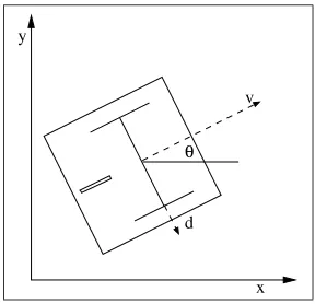
Consider the model of a simple mobile robot moving on a plane, with two independent rear motorized wheels as illustrated in Figure 1 [7, 19]:
˙
x=vcosθ+dsinθ
˙
y=vsinθ−dcosθ
˙
θ=ω ,
(56)
with v the forward velocity, ω the steering velocity, (x, y) the Cartesian position of the center of mass of the robot,θthe heading angle from the horizontal axis, andda disturbance force perpendicular to the forward direction. The system (56) is a benchmark example of systems which are not stabilizable using continuous feedback [1].
θ v
d
[image:7.595.102.246.276.415.2]x y
Figure 1: A two-wheeled drive mobile robot
Using the coordinates transformation
x1=xcosθ+ysinθ
x2=xsinθ−ycosθ
x3=θ ,
(57)
we obtain the dynamic model of system (56) in power form:
˙
x1=u1 ˙
x2=x1u2+d ˙
x3=u2 ,
(58)
whereu1:=v−ωx2, andu2:=ω.
The stabilization problem for system (58) in the ab-sence of disturbances has been studied in [19]. Using the Lyapunov function
V(t, x) =1
2(x1+ (x 2
2+x23) cost)2+ 1 2x
2 2+
1 2x
2 3 , (59)
which is a time-varying periodic function, the con-troller
u1= (x22+x23) sint−(x1+ (x22+x23) cost) (60)
u2=−2(x1+ (x22+x23) cost)(x1x2+x3) cost
−(x1x2+x3) (61)
has been designed. From the time derivative of the Lyapunov function
˙
V(t,x) =−2(x1+ (x22+x23) cost)(x1x2+x3) cost
+ (x1x2+x3)
2
−(x1+ (x22+x23) cost)2, (62)
and using La Salle Invariance Principle, it follows that in the case d = 0, the closed-loop system (58), (60), (61) is uniformly globally asymptotically stable. We consider now the case when we have a nonzero ad-ditive disturbance entering the second equation. We are interested in a particular step of the stabilization of system (58), using a discrete-time time-varying pe-riodic controller that is designed based on the approx-imate model of the system. In particular, we use the Euler model of the system (58), namely
x1(k+ 1) =x1(k) +T u1(k)
x2(k+ 1) =x2(k) +T(x1(k)u2(k) +d(k))
x3(k+ 1) =x3(k) +T u2(k).
(63)
We emphasize that the Euler approximate model satis-fies the one-step consistency we assume in constructing the results in this paper. We also need to point out that in this example we are not aiming to achieve SP-ISS for the system (58), but for the approximate model (63). However, it can be shown, following directly as what have been proved in [13, 18] for the time-invariant case, that under certain conditions the stability of the con-trolled exact discrete-time model is implied from the stability of the controlled approximate model, and the stability of the sampled-data system follows from the stability of the exact discrete-time models and bound-edness of solutions.
We then apply our result, particularly Corollary 4.1, to check the SP-ISS property of the system (63) with a controller that is designed using the idea from [19]. No-tice that for the rest of the paper, we drop the discrete-time argumentkfor simplicity.
It was shown by (62) that the derivative of the Lya-punov function (59) is negative semidefinite. Unfortu-nately, while we can apply La Salle Invariance Princi-ple for systems without disturbance, we do not have such kind of tool for systems with inputs. Hence, (59) cannot be used to show input-to-state stability of the closed-loop system.
Using a similar idea as in [8], we construct another Lyapunov function that can be used to show ISS. We use the Lyapunov function
VT =%1(V1T) +%2(V2T), %1, %2∈ K∞ , (64)
whereV1T =V and
V2T =V1T −x1(x22+x23) sint , (65)
with >0 sufficiently small to guarantee thatVT ≥0.
(63) and (64) it is easy to show that conditions (5) and (7) hold.
The Lyapunov difference ∆VT is obtained as follows:
∆VT(k, x) =VT(k+ 1, FT)−VT(k, x)
= (x1(k+ 1) + (x22(k+ 1) +x23(k+ 1)) cos((k+ 1)T))2
+x2(k+ 1)2+x3(k+ 1)2
−x1(k+ 1)(x22(k+ 1) +x23(k+ 1)) sin((k+ 1)T)
−(x1(k) + (x22(k) +x23(k)) cos(kT))2−x2(k)2
−x3(k)2+x1(k)(x22(k) +x23(k)) sin(kT)
=x1+T u1+ ((x2+T(x1u2+d))2+ (x3+T u2)2)
×cos((k+ 1)T)2−(x1+ (x22+x23) cos(kT))2
+ (x2+T(x1u2+d))2−x22+ (x3+T u2)2−x23
−(x1+T u1)
(x2+T(x1u2+d))2+ (x3+T u2)2
×sin((k+ 1)T) +x1(x22+x23) sin(kT).
Assuming that the sampling period T is sufficiently small (0< T <1), we use the following approximation
cos((k+ 1)T)−cos(kT)≈Tsin(kT)≈O(T2), (66) sin((k+ 1)T)−sin(kT)≈Tcos(kT)≈O(T). (67)
Assume also that is sufficiently small ( = O(T)). The Lyapunov difference can then be written as
∆VT(k, x)
≈2T u1
x1+ (x22+x23) cos((k+ 1)T) + 2T(x1x2+x3)
×u2cos((k+ 1)T)− 2(x
2
2+x23) sin((k+ 1)T)
+ 2T u2(x1x2+x3)
1−x1sin((k+ 1)T)
+ 2(x1+ (x22+x32) cos((k+ 1)T)) cos((k+ 1)T)
+ 2T dx2
1 + 2(x1+ (x22+x23) cos((k+ 1)T))
×cos((k+ 1)T)+O(T2).
Applying a discrete-time controller
u1T =−(x1+ (x22+x23) cos((k+ 1)T))
−2T(x1x2+x3)u2cos((k+ 1)T)
+ 2(x
2
2+x23) sin((k+ 1)T)
(68)
u2T =−(x1x2+x3)
1−x1sin((k+ 1)T)
+ 2(x1+ (x22+x23) cos((k+ 1)T))
×cos((k+ 1)T),
(69)
that is very similar to (60), (61), we will show that the closed-loop system (63),(68),(69) is SP-ISS. Sub-stituting (68), (69) into the Lyapunov difference, we
obtain
∆VT(k, x)
≤ −2T 2((sin((k+ 1)T))2+a)h(x1x2+x3)2x21
+(x 2 2+x23)2
4
i
−2T(x1+ (x22+x23) cos((k+ 1)T))2
−2T(x1x2+x3)2
2(x1+ (x22+x23) cos((k+ 1)T))
×cos((k+ 1)T) + 12
+ 2T dx2
2(x1+ (x22+x23) cos((k+ 1)T))
×cos((k+ 1)T) + 1+O(T2),
after adding a small positive offseta <<< T to avoid the first term on the right-hand side of the inequality to become zero at (k+ 1)T =iπ, i ∈N. Finally, we
use Young’s inequality to arrive at
∆VT(k, x)≤ −T(M1|x1|2+M2|x2|4+M3|x3|4)
+T M4|d|2+O(T2),
withMi>0, i∈ {1,· · · ,4}. Therefore, it is obvious
that (6) holds and hence the closed-loop discrete-time model (63),(68),(69) is SP-ISS. Moreover, notice that the Lyapunov function VT is a periodic function with
period 2π, the same as the period of the closed-loop system (63),(68),(69).
5 Summary
We have presented a converse Lyapunov theorem for ISS for parameterized discrete-time time-varying tems. We have considered the ISS property of the sys-tems in a semiglobal practical sense, which appears naturally in sampled-data design. We have also pre-sented an application of our result to discrete-time time-varying periodic systems. Finally, by the pro-vided example, we have illustrated the usefulness of our results from a practical point of view.
References
[1] R. W. Brockett. Asymptotic stability and feedback stabilization. In R. W. Brockett, R. S. Millman, and H. J. Sussmann, editors,Differential Geometric Control Theory, pages 181–191. Birkhauser, Boston, 1983.
[2] J. M. Coron. Global asymptotic stabilization for controllable systems without drift.Math. of Control Signals and Systems, 5:295–312, 1992.
[4] J. M. Godhavn and O. Egeland. A Lyapunov ap-proach to exponential stabilization of nonholonomic systems in power form. IEEE Trans. Automat. Contr., 42:1028–1032, 1997.
[5] Z. P. Jiang and Y. Wang. Input-to-state stabil-ity for discrete-time nonlinear systems. Automatica, 37:857–869, 2001.
[6] Z. P. Jiang and Y. Wang. A converse Lyapunov the-orem for discrete-time systems with disturbances.
Systems and Control Letters, 45:49–58, 2002. [7] I. Kolmanovsky and N. H. McClamroch.
Devel-opments in nonholonomic control problems. IEEE Control Systems Magazine, 15(6):20–36, 1995. [8] D. S. Laila and D. Neˇsi´c. Changing supply rates for
input-output to state stable discrete-time nonlinear systems with applications. Automatica, 39:821–835, 2003.
[9] D. S. Laila, D. Neˇsi´c, and A. R. Teel. Open and closed loop dissipation inequalities under sampling and controller emulation.European Journal of Con-trol, 8:109–125, 2002.
[10] Y. Lin. Input to state stability with respect to noncompact sets. In 13th IFAC World Congress, pages 73–78, San Francisco, 1996.
[11] Y. Lin, E. D. Sontag, and Y. Wang. A smooth con-verse Lyapunov theorem for robust stability. SIAM J. Contr. Opt., 34:124–160, 1996.
[12] R. T. M’Closkey and R. M. Murray. Exponen-tial stabilization of driftless nonlinear control sys-tems using homogeneous feedback. IEEE Trans. Automat. Contr., 42:614–628, 1997.
[13] D. Neˇsi´c and D. S. Laila. A note on input-to-state stabilization for nonlinear sampled-data sys-tems. IEEE Trans. Automat. Contr., 47:1153–1158, 2002.
[14] D. Neˇsi´c and A. Loria. On uniform asymptotic sta-bility of time-varying parameterized discrete-time cascades. IEEE Trans. Automat. Contr., 49, June, 2004.
[15] D. Neˇsi´c and A. R. Teel. Input-to-state stability for nonlinear time-varying systems via averaging.Math. Control, Signals and Systems, 14:257–280, 2001. [16] D. Neˇsi´c and A. R. Teel. A framework for
stabi-lization of nonlinear sampled-data systems based on their approximate discrete-time models. accepted in IEEE Trans. Automat. Contr., 2004.
[17] D. Neˇsi´c, A. R. Teel, and P. Kokotovi´c. Sufficient conditions for stabilization of sampled-data nonlin-ear systems via discrete-time approximations. Sys-tems and Control Letters, 38:259–270, 1999. [18] D. Neˇsi´c, A. R. Teel, and E. Sontag. Formulas
relatingKLstability estimates of discrete-time and sampled-data nonlinear systems. Systems and Con-trol Letters, 38:49–60, 1999.
[19] J. B. Pomet. Explicit design of time-varying stabi-lizing control laws for a class of controllable systems without drift. Systems and Control Letters, 18:147– 158, 1992.
[20] E. D. Sontag. Smooth stabilization implies co-prime factorization. IEEE Trans. Automat. Contr., 34:435–443, 1989.
[21] E. D. Sontag. Feedback stabilization of nonlinear systems. In M. A. Kaashoek et al., editor, Robust Control of Linear Systems and Nonlinear Control, Proceedings of the Internat. Symp. MTNS-89, pages 61–81. Birkhauser, 1990.
[22] E. D. Sontag. The ISS philosophy as a unifying framework for stability-like behaviour. In A. Isidori, F. Lamnabhi-Lagarrigue, and W. Respondek, edi-tors, Nonlinear Control in the Year 2000, Lecture Notes in Control and Information Sciences, vol-ume 2, pages 443–468. Springer, Berlin, 2000. [23] E. D. Sontag and Y. Wang. On characterizations
of the input-to-state stability property.Systems and Control Letters, 24:351–359, 1995.
[24] O. J. Sordalen and O. Egeland. Exponential sta-bilization of nonholonomic chained systems. IEEE Trans. Automat. Contr., 40:35–49, 1995.
[25] A. M. Stuart and A. R. Humphries. Dynamical Systems and Numerical Analysis. Cambridge Univ. Press, New York, 1996.