Inductance and resistance calculations for a pair of rectangular conductors

Inductance and resistance calculations for a pair of

rectangular conductors

K.F. Goddard, A.A. Roy and J.K. Sykulski

Abstract: Various semi-analytical and numerical calculations to compute the inductance and resistance of a pair of rectangular conductors are reviewed. The DC inductance of infinitely thin strips and strips of finite thickness are specifically considered. In the former case, the inductance is computed using theT-Omethod, whereas in the latter case it is computed by direct integration using Maple. In both cases, the results are checked using finite element analysis. It is also shown how the DC inductance of three strips may be computed using the method of superposition of solutions. Conformal mapping theory is used to obtain the inductance of a pair of infinitely conducting strips. Infinitely thin strips and strips of finite thickness are considered and the inductance is compared against results obtained using finite element analysis. A method of estimating the resistance of the strips is described which is expected to give useful results when the skin depth is small in relation to the thickness of the strips.

1 DC inductance of a pair of infinitely thin strip conductors

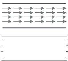
When the current distribution is known, the inductance can be obtained using theT-Omethod. The field is modelled as the sum of two components such thatH ¼Tþ rO. The vector field Tmust satisfy r T¼J. For the geometry shown in Fig. 1, this is most easily achieved by setting

Tx¼I/w in the space between the conductors and zero elsewhere.

The scalar potential field O is defined to ensure that r.B¼0. When the permeability is uniform, the fieldrOis obtained by integrating the field of magnetic polarity sources located wherer.Ta0. These fields are described in Fig. 2.

For anyT–Osolution, the inductive energy is given by 1

2I

2_L¼1

2 ZZ

T:Bdv

The inductance per unit length is obtained by integratingBx

over the rectangular area between the strips and dividing by

wI.The flux due to the vector fieldTism0Is/wbut there is a

negative contribution from the fieldrO.

The inductance per unit length (L) is then given by:

L¼ 1

wI

Z w

x¼0

Z s

y¼0

m0Tx4 Z y

h¼0

m0Tx

2p

x x2_þh2dh

dy dx

¼m0s

w

2m₀

w2_p

Z w

x¼0

Z s

y¼0

tan1 y x dy dx

Evaluating the integrals we obtain:

L¼m0s

w

2m0

p

s

2_{lnð1þ ðw=sÞ}2

Þ 4w2

(

þstan

1_ðs=wÞ

w

lnð1þ ðs=wÞ2Þ 4

)

ð1Þ

In the limit whens/wis large (1) becomes:

L¼m0

p ln

s

wþ

3 2

Figure 3 shows that whens4wa reasonable approximation is obtained using the simpler formula. Large separation s

w

I

−I Bx y

x

Fig. 1 Pair of conducting strips carrying currents I and –I

+ + + + _

_ _ _

Fig. 2 The vector fieldTand the sources of the conservative field

rO

The authors are with the School of Electronics and Computer Science, University of Southampton, Southampton, UK

E-mail: [email protected]

r IEE, 2005 (contents include material subject to r Crown Copyright 2004 Dstl)

IEE Proceedingsonline no. 20041058

approximations are also available for conductors of other shapes and a range of frequencies[1].

2 DC inductance of a pair of rectangular conductors

The DC inductance of a pair of rectangular conductors of finite thickness may be obtained as follows. In general the vector potential at any point (u,v) is given by:

Az¼ m₀

2p ZZ ₁

2lnððxuÞ 2

þ ðyvÞ2ÞJzðx;yÞdx dy

and the inductance is given by L¼RRA:Jdu dv=I2_{. The} total inductance of two conductors in series is given by

L¼L1þL2þ2M

where L1 and L2 are the self-inductances of the two

conductors andMis the mutual inductance between them. SinceAis obtained from a double integral,Lis given by a quadruple integral. For the self-inductance of a rectan-gular conductor of dimensions w and t, this quadruple integral can be reduced to a double integral using:

Z L

0

Z L

0

fðjstjÞds dt¼2 Z L

0

Lu

ð ÞfðuÞdu

whereu¼ jstj. Hence, the self-inductance is given by

L1¼L2¼

m₀

2p4 Z w

0

wp

w2

Z t

0 tq

t2 1 2lnðq

2_þp2_{Þdq dp}

wherep¼7xu7andq¼7yv7.

The calculation for mutual inductance M has less symmetry; hence, M is given by the sum of two double integrals. For the simple geometry in Fig. 4,Mis given by

M ¼m0 2p2

Z w

0

wp

w2

Z t

0 tq

t2 1

2lnððsþqÞ 2

þp2Þ

þ1

2lnððsqÞ

2_þp2_Þ

dq dp

where p¼7xu7 and s7q¼7yv7. The integrals for L1

andMwere evaluated using Maple and combine to give:

L¼ðm0=ð24pw2t2ÞÞ½16ðt3ww3tÞtan1ðt=wÞ

8pt3wþ16ðw3ss3wÞtan1ðw=sÞ ððsþtÞ4_6w2_ðsþtÞ2

þw4ÞlnððsþtÞ2þw2Þ ððstÞ46w2ðstÞ2þw4ÞlnððstÞ2þw2Þ þ8ðwðsþtÞ3w3ðsþtÞÞtan1ðw=ðsþtÞÞ þ8ðwðstÞ3w3ðstÞÞtan1_ðw=ðstÞÞ

þ2ðstÞ4lnðstÞ þ2ðsþtÞ4lnðsþtÞ 4t4lnðtÞ 4s4lnðsÞ 4w4lnðwÞ

þ2ðw46w2t2þt4Þlnðt2þw2Þ

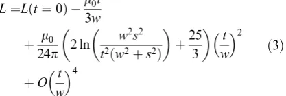
þ2ðw46w2s2þs4Þlnðs2þw2Þ: ð2Þ Figure 5 shows the DC inductance againsts/wfor various ratios of t/w. Also shown on this graph is the inductance obtained from (1) for infinitely thin strips. The similar shape of the graphs suggests that the inductance may be expressed in relation to (1). Indeed, when the formula is expanded in terms oft/wwe obtain:

L¼Lðt¼0Þ m0t 3w

þ m0 24p 2 ln

w2_s2 t2_ðw2_þs2_Þ

þ25 3

_t

w 2

þO t

w 4

ð3Þ

For the range of data plotted in Fig. 5, this expression agrees to within 0.3% of the exact formula given in (2).

The exact formula was checked against a series of finite element models and found to agree to four significant figures. This result gives a high degree of confidence that the analytical formula is correct.

0 1 2 3 4 5 6 7 8 9

0 0.5 1.0 1.5

s /w

inductance

L

, H/m (

×

10

−

7)

approximation T-Omega

Fig. 3 Comparison of inductance calculated using the T-Omethod with the large separation approximation

(x,y ) (u,v )

s

w

t

Fig. 4 Position of points in two rectangular conductors

t /w

0 1 2 3 4 5 6 7 8

0 0.2 0.4 0.6 0.8 1.0 1.2 1.4 1.6

s /w

DC inductance, H/m (

×

10

−

7) 0 0.1 0.2 0.5 1.0

3 DC inductance of a system of three strips

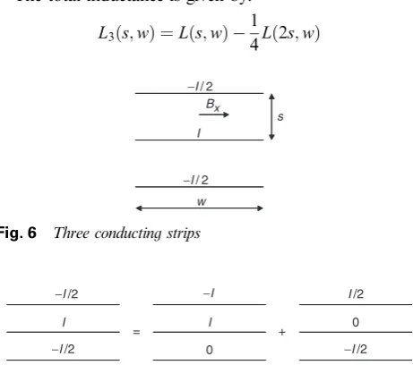
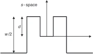
The DC inductance of the three-strip configuration in Fig. 6 is obtained as follows.

The magnetic field may be obtained from the super-position of two simpler fields, as illustrated in Fig. 7. The contribution of each of those fields to the inductance may be obtained from the earlier analysis.

The total inductance is given by:

L3ðs;wÞ ¼Lðs;wÞ 1

4Lð2s;wÞ

whereL3is the inductance for the three strips andLis the

inductance for the two strips, using (1).

An expression for the DC inductance of three strips of finite thickness may be found by using values ofLfrom (2) or (3). In this case, the total inductance is given by:

L3ðs;w;tÞ ¼Lðs;w;tÞ 1

4Lð2s;w;tÞ

4 Inductance of a pair of infinitely thin, infinitely conducting strips

This calculation was performed using the composition of two conformal mappings. The first of these is the Jacobian elliptic function, which maps a rectangle in complex z-space, for which the inductance is easily calculated, onto the upper half plane as indicated in Fig. 8. This function, denoted byw¼sn(z,k), is defined as the inverse of the function ellipticF(w,k) [2]. The function has the following properties:

snðK;kÞ ¼1; snðKþiK0;kÞ ¼1=k; snðK;kÞ ¼ 1;and snðKþiK0;kÞ ¼ 1=kwhereKandK0 are functions ofk:

Figure 9 shows the mapping of the rectangle fork¼0.5. The mapping z¼F(w)¼ellipticF(w,k), which may be derived from the Schwartz-Christoffel transformation [2],

is given by:

z¼FðwÞ ¼

Z w

0

dv

ffiffiffiffiffiffiffiffiffiffiffiffiffiffiffiffiffiffiffiffiffiffiffiffiffiffiffiffiffiffiffiffiffiffiffiffiffi

ð1v2_Þð1k2_v2_Þ

p

Having mapped the sides of the rectangle to the real axis it now remains to map the real axis in w-space to the geometry matching the two strips ins-space. This mapping, denoted by s¼p(w), is also found from the Schwartz-Christoffel transformation and is given by:

s¼pðwÞ ¼

Z w

0

ðtþbÞðtbÞdt

ffiffiffiffiffiffiffiffiffiffiffiffiffiffiffiffiffiffiffiffiffiffiffiffiffiffiffiffiffiffiffiffiffiffiffiffiffiffiffiffiffiffiffiffiffiffiffiffiffiffiffiffiffiffi

ðtþaÞðtþcÞðtcÞðtaÞ

p

Rearranging the integral we find that:

pðwÞ ¼ cb 2

c

ellipticF w a;

a c

cellipticE w a;

a c

where

ellipticEðw;kÞ ¼

Z w

0

ffiffiffiffiffiffiffiffiffiffiffiffiffiffiffiffi 1k2_t2 1t2

r

dt

The constantsa,bandcrefer to points on the real axis in

w-space; point b is mapped to the corner of the strip whereas pointsaandcare both mapped to a point midway along the side of the strip. The mapping is illustrated schematically in Fig. 10.

To ensure that, whenw¼sn(z,k), the conducting surfaces map to two opposite sides of the rectangle, we must set

c¼1 and a¼1/k. The condition p(a)¼p(1) means that b

may be expressed as a function ofa.We find that:

b2¼½a2ðellipticKð1=aÞ ellipticEða;1=aÞ þellipticEð1;1=aÞ þellipticFða;1=aÞÞ=

½ellipticFða;1=aÞ ellipticKð1=aÞ

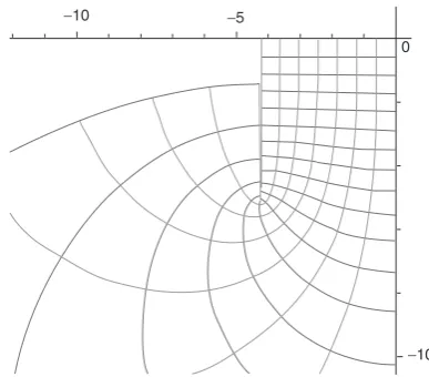
Sinceaandbare functions ofk, the mappings¼p(sn(z,k)) can be calculated for any k. Figure 11 illustrates this mapping fork¼0.1.

w

−I / 2

−I / 2

I

s B_x

Fig. 6 Three conducting strips

I /2

−I /2 −I /2

−I /2

−I

0

I

0

I

= +

Fig. 7 Use of superposition to obtain the inductance of a three-strip circuit

−K + iK ′

−K − −1

K + iK ′

K 1 1

k

z w = sn (z,k )

1

k

Fig. 8 The mapping sn (z,k)

−6 −4 −2 0 ₂

2

4 4

6 6

Fig. 9 Contours of vector and scalar magnetic potential under the map sn z

c b a

−a−b−c

w s

p (b )

p (−b )

p (−a ) = p (−c ) p (a ) = p (c )

The ratio of separation to width in s-space is given by: sep=width¼ <ðpðbÞÞ=IðpðbÞÞ ð4Þ

The value of k that satisfies (4) was found using the secant algorithm. The inductance is then found from the ratio of the side lengthsKandK0of the rectangle, which are found fromK ¼Fð1ÞandiK0¼Fð1=kÞ Fð1Þ.

Since ellipticK(k) is defined by:

ellipticKðkÞ ¼

Z 1

0

dv

ffiffiffiffiffiffiffiffiffiffiffiffiffiffiffiffiffiffiffiffiffiffiffiffiffiffiffiffiffiffiffiffiffiffiffiffiffi

ð1v2_Þð1k2_v2_Þ

p

it is clear thatK¼ellipticK(k) and

Fð1=kÞ ¼1

kellipticK 1 k :

It can be shown[3]that, for9k9o1: 1

kellipticK 1

k ¼ellipticKðkÞ iellipticKðk

0_Þ

wherek0¼pffiffiffiffiffiffiffiffiffiffiffiffiffi1k2_{. Hence, the inductance is given by:}

L¼m₀K

K0¼m0

ellipticKðkÞ

ellipticKðk0_Þ ð5Þ

A method of evaluating ellipticK(k) for9k9o1 is given in [4], and described as follows. We begin with the triplet of numbers:

l0¼1; m0¼

ffiffiffiffiffiffiffiffiffiffiffiffiffi 1k2 p

; n0 ¼k

Successive iterations ofli,miandniare found by taking:

li¼

1

2ðli1þmi1Þ mi¼

ffiffiffiffiffiffiffiffiffiffiffiffiffiffiffiffiffi

li1mi1

p

ni¼

1

2ðli1mi1Þ

Convergence is achieved whenni0 and

ellipticKðkÞ ¼ p 2li

4.1

Results

The inductance, obtained from (5) is shown in Fig. 12, and compared with the DC inductance obtained from (1). For large separations the difference between these two induc-tance values tends to a constant value ofm₀ð1:5lnð4ÞÞ=p.

The high-frequency inductance estimates obtained using the above semi-analytical method were compared with values obtained using finite element analysis and found to agree to within 0.2%. These finite element models use boundary conditions to represent the conductors. A fixed value of flux is imposed between the go and return conductors and the inductance per unit length is calculated using:

L¼f2 ZZ

B:HdA

5 Inductance of infinitely conducting strips of finite thickness

When the strips have a finite thickness, the mappingp(w) is more complicated, since the pointbat the edge of the strip has been replaced by a pair of points b1 and b2. The

mapping, which is illustrated in Fig. 13, is given by the integral:

s¼pðwÞ ¼

Z ffiffiffiffiffiffiffiffiffiffiffiffiffiffi

wþb1

p _{ffiffiffiffiffiffiffiffiffiffiffiffiffiffi} wþb2

p _{ffiffiffiffiffiffiffiffiffiffiffiffiffiffi} wb2

p _{ffiffiffiffiffiffiffiffiffiffiffiffiffiffi} wb1 p

ffiffiffiffiffiffiffiffiffiffiffiffi

wþa p ffiffiffiffiffiffiffiffiffiffiffiffi

wþc p _{ffiffiffiffiffiffiffiffiffiffiffiffi}

wc

p _{ffiffiffiffiffiffiffiffiffiffiffiffi}

wa

p dw

Unfortunately, due to the complicated nature of this integral, we have been unable to find an explicit expression forp(w). The integration between consecutive points on the real axis can, however, be performed numerically, making appropriate substitutions to remove the singularities in the denominator.

Suppose, for example, we wish to compute:

pðb2Þ pðcÞ ¼

Z b2

c

ffiffiffiffiffiffiffiffiffiffiffiffiffiffiffiffiffiffiffiffiffiffiffiffiffiffiffiffiffiffiffiffiffiffiffiffiffiffi

ðw2_b2

1Þðw2b22Þ

ðw2_a2_Þðw2_c2_Þ

s

dw

¼

Z b2

c

gðwÞ

ffiffiffiffiffiffiffiffiffiffiffiffiffiffi

wb2

wc

r

dw

−10

−10 −5

0

Fig. 11 Typical map showing contours of vector potential and scalar magnetic potential. Only one-quarter of the model is shown here

0 1 2 3 4 5 6 7 8 9

0 0.2 0.4 0.6 0.8 1.0 1.2 1.4 1.6

DC AC

s /w

inductance

L

, H/m (

×

10

−

7)

Fig. 12 Inductance as a function of separation/width

p (−b ₁)

p (−a ) p (−c ) p (c ) p (a )

p (−b ₂) p (b ₂) p (b ₁)

−a−b 1−b 2−c c b 2 b 1 a

width/2

spacing thickness

w -space s -space

where

gðwÞ ¼

ffiffiffiffiffiffiffiffiffiffiffiffiffiffiffiffiffiffiffiffiffiffiffiffiffiffiffiffiffiffiffiffiffiffiffiffiffi

ðw2_b2

1Þðwþb2Þ

ðw2_a2_ÞðwþcÞ

s

The singularities at the ends of the integration range may be removed using the substitution:

w¼cþb2

2

b2c 2

cosy

This gives

pðb2Þ pðcÞ ¼iðb₂cÞ

Z p

0

gðwÞcos2 y 2 dy Numerical integration with respect toyis now straightfor-ward. The other integrals were transformed using similar substitutions. A ‘black box’ function was constructed to compute the image ins-space of the input vector (a,b2,b1,

c) in w-space. This function is used by a Matlab optimisation function to find the values ofa, b2,b1andc

which give rise to the given geometry. Having obtained the values of a and c, the inductance is then found using (5) withk¼c/a.

5.1

Results

The above method was used to estimate the inductance for a range of values of width, separation and thickness. These results were compared with those obtained from finite element analysis and found to be in good agreement; the discrepancies were found to be less than 0.1%.

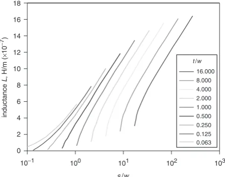
Figure 14, which is the high-frequency AC analogue of Fig. 5, shows the inductance as a function ofs/wfor various ratios of t/w. When s/w is large, the inductance shows logarithmic dependence on s/w as predicted by the large separation models[1]. As the gap between the conductors (s–t) tends to zero the inductance also tends to zero. For very small gaps, the inductance may be approximated by

m0(s–t)/w. However, the curves rapidly depart from this

asymptote as the separation increases. This behaviour is illustrated in Fig. 15.

6 Calculation of the losses

The losses are obtained from the integral of the Poynting vector around the surface of the conductor which gives the power flow into the conductor, i. e.:

power flow¼

a

For the 2D case considered:

Hz¼0 hence ðEHÞ:^nn¼EzHsurf and

R¼

R H

EzHsurfds

dt

R

I2_dt

where the time integrals are taken over a full period of the current waveform. If the skin depth is small in relation to the dimension of the rectangle a reasonable approximation can be obtained by assuming that EzandHsurfare related

by a 1D diffusion equation. If it is also assumed that the current waveform is sinusoidal, we find that:

R

EzHsurfdt

R

H2

surfdt

¼ 1

sD

and hence

R¼ 1

s D I _H2

surf

I2 ds

The integralRH2surfdsins-space may be converted into an

integral along the real axis in w-space. If O denotes the scalar magnetic potential:

Hsurf¼ dO

ds and

Z

H_surf2 ds¼

Z _dO

dw

_ds

dw

2 _ds

dw dw

¼ dO

dz

2Z

dz dw

2,_ds

dw dw

As before, values of c, b2, b1 and a are computed

numerically to produce the given geometry. Note that: dO

dz ¼

I 2jzðaÞ zðcÞj

and

dz

dw¼

1

ffiffiffiffiffiffiffiffiffiffiffiffiffiffiffiffiffiffiffiffiffiffiffiffiffiffiffiffiffiffiffiffiffiffiffiffiffiffi

ðw2_a2_Þðw2_c2_Þ

p

!

from which it can be seen that:

zðaÞ zðcÞ

j j ¼1

aellipticK

ffiffiffiffiffiffiffiffiffiffiffiffiffiffiffiffiffiffiffiffiffi 1ðc=aÞ2

q

t /w

0 2 4 6 8 10 12 14 16 18

10−1 100 101 102 103

16.000 8.000 4.000 2.000 1.000 0.500 0.250 0.125 0.063

s /w

inductance

L

, H/m (

×

10

−

7)

Fig. 14 L as a function of s/w for various t/w

0 1 2 3 4 5 6 7 8 9 10

0 0.4 0.8 1.2 1.6

(s − t )/w

inductance

L

, H/m (

×

10

−

7)

t /w

16.000 8.000 4.000 2.000 1.000 0.500 0.250 0.125 0.063 0 asymptote

Also

ds

dw¼

ffiffiffiffiffiffiffiffiffiffiffiffiffiffiffiffiffiffiffiffiffiffiffiffiffiffiffiffiffiffiffiffiffiffiffiffiffiffi

ðw2_b2

1Þðw2b22Þ

ðw2_a2_Þðw2_c2_Þ

s

Therefore

dz dw

2, ds dw¼

1

ffiffiffiffiffiffiffiffiffiffiffiffiffiffiffiffiffiffiffiffiffiffiffiffiffiffiffiffiffiffiffiffiffiffiffiffiffiffiffiffiffiffiffiffiffiffiffiffiffiffiffiffiffiffiffiffiffiffiffiffiffiffiffiffiffiffiffiffiffiffiffiffiffiffiffiffi

ðw2_a2_Þðw2_c2_Þðw2_b2

1Þðw2b22Þ

q 0 B @

1 C A

ð6Þ Hence, the losses are given by:

1

sD Z

surf

H_surf2 ds¼ 1

sD

dO

dz

2Z a

c

dz dw

2,

ds

dw dw

where the integrand on the right-hand side is given by (6). The integration in w-space is performed along a contour representing the surface of the conductor, i.e. betweencand

a. The integral is evaluated in three pieces using the technique described in Section 5 to remove the singularities. In the case where the width is large compared to the separation, the ratio a/c is very large. This may cause substantial numerical errors in the evaluation of the integrals. An alternative geometry that avoids these inaccuracies is given in Fig. 16. A rectangular region between the conductors is left untransformed; hence, allowance must be made for the current and the associated losses in this region. If this method is used, it is important thatdis sufficiently large that the field at the interface may be considered uniform.

Figure 17 showswsDRas a function ofs/w. These results were obtained using the above semi-analytical method. When s/w - 0, Hsurf-I/w and so

R

H2

surfdl=I2 -1/w.

When s/w-N, RH_surf2 dl=I2 tends to the value for an isolated strip with the same dimensions.

These results were compared against those obtained using finite element analysis. Initially, the finite element package was used to integrateH2around the surface of the conductor. In most cases, this yielded a result within 2.5% of the value obtained using the above method. However, in a few cases, the discrepancies were substantially larger.

To confirm that the largest errors arise in the integration ofH2around the conductor in the finite element model, an alternative method was developed to evaluate RH2

surfdl

within a short distance r of the corner. This integral was evaluated using the values of vector potential on an arc at radiusrfrom the corner. This approach uses the conformal mappings¼s0+Aw3/2where9A9¼rands0is the position

of the corner. From Fourier analysis of the vector potential on the arc of radiusr, a Taylor series is defined representing the potential inw-space. An analytical function was defined which gives RH_surf2 dl in terms of the coefficients of this Taylor series and the radiusr. Using this method, the finite element results agree with the results obtained from the semi-analytical method to within 0.3%.

7 Conclusions

For a pair of rectangular conductors it is possible to obtain an analytical expression for the DC inductance by direct integration. A good approximation to this result, which agrees to within 0.3%, is obtained by expanding this expression in powers oft/w. An analytical expression for the DC inductance of three strips may be obtained using superposition of solutions.

The high-frequency AC resistance and inductance can be estimated using conformal mapping theory without requir-ing finite element software. The position of the poles and zeros that define the conformal mapping are obtained using numerical integration and optimisation functions. The inductance can be computed directly from these positions, while the resistance must be calculated by numerical integration of H2surf. The accuracy of the estimates of the

inductance and RH_surf2 dl obtained by this method was checked by comparison with results obtained using finite element analysis. Once measures were taken to control errors in RH2

surfdlaround the corners of the finite element model, the two methods agree to a high degree of accuracy.

8 References

1 Goddard, K.F., Roy, A.A., and Sykulski, J.K.: ‘Inductance and resistance calculations for isolated conductors’,IEE Proc., Sci., Meas.

Technol., (in print)

2 Nehari, Z.: ‘Conformal mappings’ (McGraw-Hill, New York, 1952) 3 Grover, F.W.: ‘Inductance calculations, working formulas and tables’

(Dover, New York, 1962)

4 Abramovitz, M., and Stegun, I.A.: ‘Handbook of mathematical functions’ (Dover, New York, 1965)

s -space

d w /2

Fig. 16 A simpler type of geometry

10−3 10−2 10−2

10−1 10−1

100 100

101 102 103

s /w

R

σ∆

w

t /w 0.0625 0.1250 0.250 0.5 1 2 4 8 16