Journeys in Big Data statistics
Ian L. Dryden and David J. Hodge
School of Mathematical Sciences, University of Nottingham, UK.
Abstract
The realm of big data is a very wide and varied one. We discuss old, new, small and big data, with some of the important challenges including dealing with highly-structured and object-oriented data. In many applications the objective is to discern patterns and learn from large datasets of historical data. We shall discuss such issues in some transportation network applications in non-academic settings, which are naturally applicable to other situations. Vital aspects include dealing with logistics, coding and choosing appropriate statistical methodology, and we provide a summary and checklist for wider implementation.
1
A new natural resource
We will be the first to admit that it is difficult to keep up. How can you expect someone who is trained in dealing with datasets of n = 30observations withp = 3variables to suddenly cope with a 100K-fold increase ofn = 3000000observations and p = 300000for example, or even worse? Everything has to change. Summarizing a dataset becomes a major computational challenge and p-values take on a ludicrous role where everything is significant. Yet dealing with a wide range of sizes of datasets has become vital for the modern statistician.
Virginia Rometty, chairman, president and chief executive officer of IBM said the following at North-western University’s 157th commencement ceremony in 2015:
What steam was to the 18th century, electricity to the 19th and hydrocarbons to the 20th, data will be to the 21st century. That’s why I call data a new natural resource.
The need to make sense of the huge rich seams of data being produced underlines the great importance of Statistics, Mathematical and Computational Sciences in today’s society. But what is ‘new’ about data? Data has been used for centuries, for example data collected on the first bloom of cherry blossoms in Kyoto, Japan starting in 800AD and now highlighting climate change (Aono, 2017); Gauss’s meridian arc measurements in 1799 used to define the metre (Stigler, 1981); and Florence Nightingale’s 1859 mortality data and graphical rose diagram presentation on causes of death in the Crimean War leading to modern nursing practice (Nightingale, 1859). All of these old, small datasets are at the core of important issues for mankind, so it is not the data or its importance but the size, structure and ubiquity of data that is new.
used to be the realm of careful asymptotic theory or thought experiments, but in reality one often does encounter largennow in practice.
Two possible routes to practical inference are conditioning and sampling. Conditioning on a small win-dow of values of a subset of covariates will very quickly reduce the size of data available as the number of covariates increases, due to the curse of dimensionality. Such small subsets of the dataset can be used to estimate predictive distributions conditional on the values of the covariates, leading to useful predic-tions. We give some further detail below in a case study from the transport industry. Sampling sensibly on the other hand is a more difficult task. Although it is straightforward to sample at random of course, given the inherent biases in most big data one needs to carry out sampling to counteract the bias in the data collection.
A further aspect of the avalanche of new data being available is that it is often highly-structured. For ex-ample, large quantities of medical images are routinely collected each day in hospitals around the world, each containing highly-complicated structured information. The emerging area of Object Oriented Data Analysis (Marron and Alonso, 2014) provides a new way of thinking of statistical analysis for such data. Examples of object data include functions, images, shapes, manifolds, dynamical systems, and trees. The main aims of multivariate analysis extend more generally to object data, e.g. defining a distance between objects, estimation of a mean, summarizing variability, reducing dimension to important com-ponents, specifying distributions of objects, carrying out hypothesis tests, prediction, classification and clustering.
From Marron and Alonso (2014), in any study an important consideration is to decide what are the atoms (most basic parts) of the data. A key question is ‘what should be the data objects?’, and the answer will then lead to appropriate methodology for statistical analysis. The subject is fast developing following initial definitions in Wang and Marron (2007), and a recent summary with discussion is given by Marron and Alonso (2014) with applications to Spanish human mortality functional data, shapes, trees and medical images. One of the key aspects of object data analysis is that registration of the objects must be considered as part of the analysis. In addition the identifiability of models, choice of regularization and whether to marginalize or optimize as part of the inference are important aspects of object data analysis, as they are in statistical shape analysis (Dryden and Mardia, 2016).
It is obvious that the realm of big data is a very wide and varied one. In some realms the difficulties lie with truly astronomical quantities of data which are not even feasibly stored for future retrieval, for which online algorithm development is a key area of research; whereas in other realms the challenge is in discerning patterns and learning from large datasets of historical data. We shall discuss the latter, in gen-erality, below for what can loosely be thought of as transportation network applications in non-academic settings. Many of the approaches and recommendations discussed below are naturally applicable to other applications, such as a general practice of data retention, while others related to origin-destination filtering are clearly more specific to transportation problems.
2
Case Study: transportation big data
statistical analysis on datasets harvested by businesses about their customers, to either improve customer experience or to improve business efficiency. We concern ourselves here with the challenges one will meet in embedding good practice and developing useful models for exploitation of data in businesses where perhaps even the initial data handling task has so far seemed daunting.
Studying transportation systems as networked queues has been one of the most natural approaches, borne out of the queueing theory literature of previous decades. Courtesy of advances in computing, larger and larger network problems are now attempted to be ‘solved’ or at least approximately solved. Much of the focus in recent years lies with proposing online algorithms for live traffic management. With big data, opportunities arise to try and optimize these local dynamic decision problems: of re-routing a vehicle; skipping stops (if permitted); or allocating platforms, all in light of a wealth of additional statistical information. Approaches to dynamic resource allocation laid out in (Glazebrook et al., 2014) would often benefit from a serious statistical analysis to first properly understand the dynamics of a network-based model, so that when formulating the problem in a queueing framework an appropriate level of confidence can be placed on the stochastic quantities. In particular, if you were to consider traffic management decisions on a railway surrounding the choice of platforms or use of signals outside a busy station, an effective algorithm for allocating the resource that is the station platform at a particular time can only function with a well-calibrated cost function which accounts for knock-on effects of such a decision. Possessing years of historical data during which a wealth of such decisions have been made and their consequences mapped, leads us very naturally to first want to perform some robust statistical analyses.
For statistical analyses, the natural starting point to a statistician is gaining access to the appropriate historical data. There are already two large data types of interest, customer-centric journey counting or vehicle journeys. In the world of buses it is estimated that over 5 billion passenger journeys occur each year in the UK (Department of Transport, UK (2016)), for example, and the alternative approach lies with vehicle logging data. For our discussion we shall concern ourselves more with logged vehicle movements, such as the approximately three million individual train movements which are logged on a given day. For both buses and trains there is far more information available than just logged movements of stops, departures, and waypoint visiting. These can include signal changes, platform assignments, detours, engine types, vehicle capacities or raw passenger numbers. A few million daily datapoints is certainly not as large as some datasets, however the ability to store and then later quickly access and filter a database over a considerable time period can still become a non-trivial challenge. The typical format of vehicle data is broken down across the regions of a country, but sometimes even individual journeys may span more than one region. Considerable data cleaning may also be required to remove duplication, to collate, and at times even resolve issues of contradictory data logged by different systems or network operators. Each logged message can also typically contain tens of covariates indicating information ranging from the current time and present location of a vehicle, to its previous location, intended destination, top speed, personal capacity, and even properties like the engine type.
expertise for later retrieval is already a positive benefit to big data thinking.
When it comes to handling large datasets some of the go-to tools of the research statistician such as the R software (R Core Team, 2017) need to be handled with care. Whilst packages exist to manage hard-ware issues such as large memory footprints, at every stage consideration needs to be given to repeated database access and careful filtering to ensure that analysis is only performed on sets of data which are not excessively large. In transport applications, this often means filtering journeys by their origin-destination pair, or for spatial analysis, aggregating datapoints over small geographical cells, for a large number of different cells. In removing all messages not directly related to vehicles travelling between a specific Origin–Destination (OD) pair one can concentrate on identifying recurrent behaviours and pat-terns. Unfortunately, in transport networks there may be other vehicles which interact with vehicles on this particular route but which do not share the same OD pair. Thus a combination of filtering approaches may be required. Many natural approaches to transport, therefore, try to model the characteristics of each individual piece of infrastructure, as a function of a range of up to fifteen or so covariates of vehicles that pass through it. This can then be used either for infrastructure assessment, or as part of live vehicle pre-diction modelling. Of more prevalent use in the business world are data visualization tools like Tableau for creating slick graphics for presentations. With big data, however, there is very often the need to have already performed some careful database filtering and covariate selection to ensure appropriately-sized and relevant datasets are used to create the visualizations.
A number of academic challenges arise when trying to use such enormous quantities of data to make single predictions, or evaluations, for example in trying to predict the future lateness of a particular ve-hicle’s on-going journey. Identification of explanatory variables, along with appreciation of the physical mechanisms will often drive an appropriate model choice to distil the enormous datasets into appropri-ate predictions or summary data. Deciding whether to chain the use of linear models across a network of (assumed) independent locations, or to attempt kernel regression methods to weight a much larger number of proximate locations for the same purpose is not always easily determined. Indeed the most flexible approach obviously lies in maintaining the ability to try as many plausible avenues as possible, without having to make compromises to accommodate the potentially overwhelmingly large numbers of datapoints that may arise without appropriate data filtering.
Any analysis of large transport datasets should therefore at the outset try and identify what geographic information is available and down to what level of granularity any modelling intends to go. The more granular the analysis the more consideration will need to be given to systematic slicing of the data. One typical approach is to store daily logs and then sequentially query the data in each log file separately, and interrogate it for data matching the chosen covariate ranges. This approach could be used either to find other vehicles of similar characteristics (such as current lateness, current location or destination) if prediction by similarity to previous conditions is intended, or if a mutli-level model is intended then the datasets can be interrogated to find all data relevant to the piece of road or track that a particular vehicle is currently on, to first characterize the infrastructure and then use this characterization in drawing some desired model inference. Anecdotally the complexity of existing methods used by network operators to predict future lateness of buses, or trains are not generally very sophisticated, often just assuming unchanging lateness. As such, relatively simple linear models based upon historical data are capable of discernable improvements in prediction accuracy.
teams across a company seeing the benefits to a more rigorous approach to data and result in more joint enterprises, particularly with regard to making future statistically qualified job appointments. This can be in particular contrast with non-big data applications because then relatively low initial overheads can discourage this collaborative approach.
One final noteworthy difficultly lies in the use of big data in live systems, for example in providing live information to customers about service status. Pure reporting of the status of vehicles in a transport net-work is not a difficult mathematical task. However, if predictions of future behaviour are being provided to enhance the customer experience then there can be a need to appropriately design analysis systems to cope with both live data input and output in a timely manner. Early identifications of such needs can help ensure that data handling and storage solutions selected are suitable. Whenever such live data is required in the field there are then also all the accompanying issues concerning data stewardship, and having suitable fallback systems if a data stream should be interupted.
In summary, in our transportation example above a number of topics that particularly arise with big data in a commercial transportation network operation setting have been discussed to highlight many of those key issues worthy of consideration. While we hear of big data exploitation almost daily in the context of the big worldwide computing companies there is still a large untapped potential from the use of statistical analysis for big data in many more established industries such as retail, transportation and manufacturing.
3
Summary and checklist
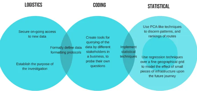
We provide a summary of the starting points for a typical investigation as follows:
• Secure on-going access to new data.
• Establish the purpose of an investigation, e.g. to identify network bottlenecks, to identify worst performing routes, to reduce emissions, to make travel time predictions etc. . .
• Establish formally the data format to use.
• Create tools to allow querying of the data by different stakeholders in a business, to probe their own questions.
• Use classification techniques to discern patterns, and rankings of routes.
• Try regression techniques over a fine geographical grid to model the effect of small pieces of in-frastructure (e.g. a particular stretch of road, bus station, railway track or station) upon the future journey of a vehicle. Decisions, however, need to be made concerning which historical data to use to make good predictions, by identifying relevant covariates.
• Implement the statistical techniques efficiently, for live usage.
A graphical checklist for a typical investigation is given in Figure 1.
Acknowledgement
Figure 1: Checklist for a typical investigation
References
Aono, Y. (2017). Japan’s cherry blossoms are emerging increasingly early. The Economist. https:// www.economist.com/blogs/graphicdetail/2017/04/daily-chart-4[Accessed: 29 Sep 2017].
Department of Transport, UK (2016). Annual Bus Statistics of Great Britain, 2016. https://www. gov.uk/government/collections/bus-statistics[Accessed: 29 Sep 2017].
Dryden, I. L. and Mardia, K. V. (2016). Statistical Shape Analysis, with Applications in R, 2nd edition. Wiley, Chichester.
Glazebrook, K. D., Hodge, D. J., Kirkbride, C., and Minty, R. J. (2014). Stochastic scheduling: a short history of index policies and new approaches to index generation for dynamic resource allocation. J. Sched., 17(5):407–425.
Hastie, T., Tibshirani, R., and Wainwright, M. (2015).Statistical Learning with Sparsity: The Lasso and Generalizations. Chapman and Hall/CRC Press, Boca Raton.
Marron, J. S. and Alonso, A. M. (2014). Overview of object oriented data analysis.Biometrical Journal, 56(5):732–753.
Nightingale, F. (1859).A contribution to the sanitary history of the British army during the late war with Russia. John W. Parker and Son, London. https://iiif.lib.harvard.edu/manifests/ view/drs:7420433$2i[Accessed: 29 Sep 2017].
R Core Team (2017). R: A Language and Environment for Statistical Computing. R Foundation for Statistical Computing, Vienna, Austria.
Stigler, S. M. (1981). Gauss and the invention of least squares.Ann. Statist., 9(3):465–474.