Automated multi stage geometry parameterization of internal fluid flow applications

Full text

(1)University of Southampton Research Repository ePrints Soton. Copyright © and Moral Rights for this thesis are retained by the author and/or other copyright owners. A copy can be downloaded for personal non-commercial research or study, without prior permission or charge. This thesis cannot be reproduced or quoted extensively from without first obtaining permission in writing from the copyright holder/s. The content must not be changed in any way or sold commercially in any format or medium without the formal permission of the copyright holders.. When referring to this work, full bibliographic details including the author, title, awarding institution and date of the thesis must be given e.g. AUTHOR (year of submission) "Full thesis title", University of Southampton, name of the University School or Department, PhD Thesis, pagination. http://eprints.soton.ac.uk.

(2) UNIVERSITY OF SOUTHAMPTON. Automated Multi-Stage Geometry Parameterization of Internal Fluid Flow Applications. Nicola Hoyle. Thesis for the degree of Doctor of Philosophy. Faculty of Engineering, Science and Mathematics School of Electronics and Computer Science. September 2006.

(3) UNIVERSITY OF SOUTHAMPTON ABSTRACT FACULTY OF ENGINEERING, SCIENCE AND MATHEMATICS SCHOOL OF ELECTRONICS AND COMPUTER SCIENCE Doctor of Philosophy by Nicola Hoyle. The search for the most effective method for the geometric parameterization of many internal fluid flow applications is ongoing. This thesis focuses on providing a generalpurpose automated parameterization strategy for use in design optimization. Commercial Computer-Aided Design (CAD) software, Computational Fluid Dynamics (CFD) software and optimizer tools are brought together to offer a generic and practical solution. A multi-stage parameterization technique for three-dimensional surface manipulation is proposed. The first stage in the process defines the geometry in a global sense, allowing large scale freedom to produce a wide variety of shapes using only a small set of design variables. Invariably, optimization using a simplified global parameterization does not provide small scale detail required for an optimal solution of a complex geometry. Therefore, a second stage is used subsequently to fine-tune the geometry with respect to the objective function being optimized. By using Kriging response surface methodology to support the optimization studies, two diverse applications, a Formula One airbox and a human carotid artery bifurcation, can be concisely represented through a global parameterization followed by a local parameterization..

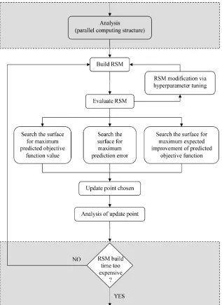
(4) Contents List of Figures. v. List of Tables. x. Nomenclature. xi. Declaration of Authorship. xiv. Acknowledgements. xv. 1 Introduction 1.1 Computer-Aided Geometric Design . . . . . . . . 1.1.1 A Brief History . . . . . . . . . . . . . . . 1.1.2 The Role of Geometry Parameterization Optimization . . . . . . . . . . . . . . . . 1.2 Background and Objective of work . . . . . . . . 1.3 Thesis Outline . . . . . . . . . . . . . . . . . . .. . . . . . . . . . . . . . . . . . . . . . . . . . . in CFD-Based Design . . . . . . . . . . . . . . . . . . . . . . . . . . . . . . . . . . . . . . .. . 5 . 7 . 12. 2 Design Optimization Methodology 2.1 An Automated System Architecture . 2.2 Geometric Parameterization . . . . . . 2.2.1 Polynomial Curves . . . . . . . 2.2.2 Bézier Curves . . . . . . . . . . 2.2.3 B-splines . . . . . . . . . . . . 2.2.4 Hicks-Henne Bump Functions . 2.3 Design of Experiments . . . . . . . . . 2.4 Computational Fluid Dynamics . . . . 2.5 Response Surface Methodology . . . . 2.6 Exploration of Reduced Design Space 2.7 Summary . . . . . . . . . . . . . . . .. . . . . . . . . . . .. . .. 1 2 2. . . . . . . . . . . .. . . . . . . . . . . .. . . . . . . . . . . .. . . . . . . . . . . .. . . . . . . . . . . .. . . . . . . . . . . .. . . . . . . . . . . .. . . . . . . . . . . .. . . . . . . . . . . .. . . . . . . . . . . .. . . . . . . . . . . .. . . . . . . . . . . .. 14 16 18 18 20 22 22 23 24 26 28 29. 3 Optimization using Response Surface Methodology 3.1 A Global Approximation . . . . . . . . . . . . . . . . . 3.1.1 Kriging . . . . . . . . . . . . . . . . . . . . . . 3.2 The Update Process . . . . . . . . . . . . . . . . . . . 3.2.1 Searching the RSM . . . . . . . . . . . . . . . . 3.2.1.1 The Predictor . . . . . . . . . . . . . 3.2.1.2 Prediction Error . . . . . . . . . . . .. . . . . . .. . . . . . .. . . . . . .. . . . . . .. . . . . . .. . . . . . .. . . . . . .. . . . . . .. . . . . . .. . . . . . .. . . . . . .. 30 30 33 33 37 37 39. ii. . . . . . . . . . . .. . . . . . . . . . . .. . . . . . . . . . . .. . . . . . . . . . . .. . . . . . . . . . . .. . . . . . . . . . . .. . . . . . . . . . . ..

(5) CONTENTS. 3.3. iii. 3.2.1.3 Expected Improvement . . . . . . . . . . . . . . . . . . . 40 3.2.1.4 Regression Term . . . . . . . . . . . . . . . . . . . . . . . 41 Summary . . . . . . . . . . . . . . . . . . . . . . . . . . . . . . . . . . . . 42. 4 An 4.1 4.2 4.3 4.4. Automated Single Stage Shape Optimization Case Study The Global Optimization of a Two-Dimensional Airbox . . . . . Design Objective . . . . . . . . . . . . . . . . . . . . . . . . . . . CFD Analysis and Optimization Strategy . . . . . . . . . . . . . Straight Diffuser . . . . . . . . . . . . . . . . . . . . . . . . . . . 4.4.1 Geometry Parameterization . . . . . . . . . . . . . . . . . 4.4.2 Results . . . . . . . . . . . . . . . . . . . . . . . . . . . . 4.5 Elbow . . . . . . . . . . . . . . . . . . . . . . . . . . . . . . . . . 4.5.1 Geometry Parameterization . . . . . . . . . . . . . . . . . 4.5.2 Results . . . . . . . . . . . . . . . . . . . . . . . . . . . . 4.6 Diffuser with Bend . . . . . . . . . . . . . . . . . . . . . . . . . . 4.6.1 Combined Geometry Parameterization . . . . . . . . . . . 4.6.2 Results . . . . . . . . . . . . . . . . . . . . . . . . . . . . 4.7 Summary . . . . . . . . . . . . . . . . . . . . . . . . . . . . . . .. . . . . . . . . . . . . .. 5 Automated Multi-Stage Shape Optimization with Deformation (AMSSOD) 5.1 Global versus Local Geometry Manipulation . . . . . . . . . . . . . 5.1.1 Non-Uniform Rational Polynomial Spline Surfaces . . . . . 5.1.2 Non-Uniform Rational B-spline Surfaces . . . . . . . . . . . 5.1.3 Partial Differential Equations . . . . . . . . . . . . . . . . . 5.1.4 Three-Dimensional Hicks-Henne Functions . . . . . . . . . . 5.1.5 Free-Form Deformation . . . . . . . . . . . . . . . . . . . . 5.1.6 Subdivision Surfaces . . . . . . . . . . . . . . . . . . . . . . 5.2 Multi-Stage Geometry Parameterization . . . . . . . . . . . . . . . 5.2.1 Stage 1 . . . . . . . . . . . . . . . . . . . . . . . . . . . . . 5.2.2 Stage 2 . . . . . . . . . . . . . . . . . . . . . . . . . . . . . 5.3 Optimization using AMSSOD . . . . . . . . . . . . . . . . . . . . . 5.4 Summary . . . . . . . . . . . . . . . . . . . . . . . . . . . . . . . . 6 AMSSOD Implemented on a Three-Dimensional Airbox 6.1 Geometry Parameterization . . . . . . . . . . . . . . . . . . 6.1.1 Stage 1 . . . . . . . . . . . . . . . . . . . . . . . . . 6.1.2 Stage 2 . . . . . . . . . . . . . . . . . . . . . . . . . 6.2 CFD Analysis . . . . . . . . . . . . . . . . . . . . . . . . . . 6.3 Results . . . . . . . . . . . . . . . . . . . . . . . . . . . . . . 6.3.1 Stage 1 with Profiled Velocity Inlet Condition . . . . 6.3.2 Stage 1 with External Domain . . . . . . . . . . . . 6.3.3 Stage 2 . . . . . . . . . . . . . . . . . . . . . . . . . 6.4 Summary . . . . . . . . . . . . . . . . . . . . . . . . . . . .. . . . . . . . . .. . . . . . . . . .. . . . . . . . . .. . . . . . . . . .. . . . . . . . . . . . . .. . . . . . . . . . . . .. . . . . . . . . .. . . . . . . . . . . . . .. . . . . . . . . . . . .. . . . . . . . . .. . . . . . . . . . . . . .. . . . . . . . . . . . .. . . . . . . . . .. . . . . . . . . . . . . .. 43 43 44 44 48 50 52 56 57 58 59 59 60 66. . . . . . . . . . . . .. 70 73 73 74 77 80 82 83 86 87 87 88 89. . . . . . . . . .. 91 91 92 94 96 97 98 104 111 121. 7 AMSSOD Implemented on a Human Carotid Artery Bifurcation 123 7.1 Geometry Parameterization . . . . . . . . . . . . . . . . . . . . . . . . . . 128.

(6) CONTENTS. 7.2. 7.3. iv. 7.1.1 Stage 1 . . . . . . . . . . . . . . . . . . . . . . . . . . . . . . . . 7.1.2 Stage 2 . . . . . . . . . . . . . . . . . . . . . . . . . . . . . . . . Results . . . . . . . . . . . . . . . . . . . . . . . . . . . . . . . . . . . . . 7.2.1 CFD Comparison of Patient and CAD Carotid Artery Bifurcation Model . . . . . . . . . . . . . . . . . . . . . . . . . . . . . . . . . Summary . . . . . . . . . . . . . . . . . . . . . . . . . . . . . . . . . . .. . 130 . 134 . 139 . 143 . 154. 8 Discussion and Conclusion 155 8.1 Hitherto... . . . . . . . . . . . . . . . . . . . . . . . . . . . . . . . . . . . . 156 8.2 Thereafter . . . . . . . . . . . . . . . . . . . . . . . . . . . . . . . . . . . . 160 A Kriging Theory 162 A.1 Maximum Likelihood . . . . . . . . . . . . . . . . . . . . . . . . . . . . . . 163 A.2 Prediction Error – A Gaussian Approach . . . . . . . . . . . . . . . . . . . 168 A.3 Expected Improvement . . . . . . . . . . . . . . . . . . . . . . . . . . . . . 174 B 3D Airbox Analysis Setup B.1 Mesh Generation . . . . . . . . . . . . . . . . . . . . . . . . . B.1.1 Internal Airbox . . . . . . . . . . . . . . . . . . . . . . B.1.2 External Flow around Airbox . . . . . . . . . . . . . . B.1.3 Reduced External Flow around Airbox . . . . . . . . . B.2 Flow Simulation . . . . . . . . . . . . . . . . . . . . . . . . . B.2.1 Internal Airbox Simulation with Uniform Inlet Profile B.2.2 Simulation Including Complete External Domain . . . B.2.3 Simulation with Prescribed Inlet Velocity Profile . . . B.2.4 Comparison of all Simulations . . . . . . . . . . . . . . B.3 Mesh Dependency Study . . . . . . . . . . . . . . . . . . . . .. . . . . . . . . . .. . . . . . . . . . .. . . . . . . . . . .. . . . . . . . . . .. . . . . . . . . . .. . . . . . . . . . .. 177 . 177 . 177 . 177 . 180 . 182 . 182 . 183 . 184 . 184 . 185. C Carotid Artery Analysis Setup 192 C.1 Automated Artery Point Cloud Analysis . . . . . . . . . . . . . . . . . . . 192 C.2 Automated Creation of New Bump Deformation . . . . . . . . . . . . . . 205 C.3 Flow Simulation . . . . . . . . . . . . . . . . . . . . . . . . . . . . . . . . 209 Bibliography. 211.

(7) List of Figures 1.1 1.2 1.3 1.4 1.5. Mechanical spline tool (illustration given by Raalamb (1691)) . . . . . . Bézier’s basic curve . . . . . . . . . . . . . . . . . . . . . . . . . . . . . . Airbox inlet (2003 season) . . . . . . . . . . . . . . . . . . . . . . . . . . Airbox positioning within the F1 car . . . . . . . . . . . . . . . . . . . . Restriction of entry area to limit engine power (see inset), seen to have been used on certain F1 cars during the pre-2006 season testing . . . . . Y-shaped artery model (left), tuning fork artery model (centre) and real artery model (right) . . . . . . . . . . . . . . . . . . . . . . . . . . . . .. . 3 . 4 . 9 . 10. 2.1 2.2 2.3 2.4 2.5. A generalised optimization strategy GEODISE system architecture . . A piecewise cubic spline . . . . . . A Bézier curve . . . . . . . . . . . Two Hicks-Henne bump functions .. . . . . .. 3.1. Kriging update process . . . . . . . . . . . . . . . . . . . . . . . . . . . . . 34. 1.6. . . . . .. . . . . .. . . . . .. . . . . .. . . . . .. . . . . .. . . . . .. . . . . .. . . . . .. . . . . .. . . . . .. . . . . .. . . . . .. . . . . .. . . . . .. . . . . .. . . . . .. . . . . .. . . . . .. . . . . .. . . . . .. . 10 . 12. Graph illustrating the dependency of Cp value with mesh density for a 2D straight walled diffuser . . . . . . . . . . . . . . . . . . . . . . . . . . . 4.2 An example of a ∼39000 cell mesh with inlet, filter and outflow positions 4.3 Validation between CFD model and Madsen et al. (1999) . . . . . . . . . 4.4 Spline parameterization of straight diffuser . . . . . . . . . . . . . . . . . 4.5 Filled contours of velocity magnitude in the whole computational domain of the symmetry half of a straight wall (top) and optimum convergentdivergent wall (bottom) diffuser (the diffuser section has been magnified to illustrate the difference in wall geometry) . . . . . . . . . . . . . . . . . 4.6 Wall shear stress values in the streamwise direction along the wall of a straight walled diffuser . . . . . . . . . . . . . . . . . . . . . . . . . . . . . 4.7 Wall shear stress values in the streamwise direction along the wall of the the convergent-divergent diffuser shown at the bottom of Figure 4.5. . . . 4.8 Filled contours of velocity magnitude in the whole computational domain of the symmetry half of a bell-shaped diffuser (the diffuser section has been magnified to show the wall shape more clearly) . . . . . . . . . . . . 4.9 Geometry parameterization shown for a Bézier curve defined centreline . . 4.10 Geometry parameterization of 2D airbox model . . . . . . . . . . . . . . . 4.11 Optimization history: 200 DoE points followed by 100 update points, further followed by a 50 point exploration in 20% of the design space . . .. 15 17 19 21 23. 4.1. v. 46 46 50 51. 54 55 55. 56 57 60 61.

(8) LIST OF FIGURES 4.12 Filled contours of velocity magnitude (top) and velocity vectors (bottom) of velocity magnitude in a design which contains no flow separation, with Cp = 0.7805 . . . . . . . . . . . . . . . . . . . . . . . . . . . . . . . . . . 4.13 Filled contours of velocity magnitude (top) and velocity vectors (bottom) of velocity magnitude in the best design after 100 update points, with Cp = 0.9316 . . . . . . . . . . . . . . . . . . . . . . . . . . . . . . . . . . 4.14 Filled contours (top) and velocity vectors (bottom) of velocity magnitude in the optimum design found having completed a 50 point concentrated exploration with Cp = 0.9658 . . . . . . . . . . . . . . . . . . . . . . . . 4.15 Filled contours (top) and velocity vectors (bottom) of velocity magnitude in a design which contains no separation with Cp = 0.9452 found during the 50 point concentrated exploration . . . . . . . . . . . . . . . . . . . 4.16 Filled contours (top) and velocity vectors (bottom) of velocity magnitude in a design with a straight upper wall and Cp = 0.9555 found during the 50 point concentrated exploration . . . . . . . . . . . . . . . . . . . . . . 5.1 5.2 5.3 5.4 5.5 5.6 5.7 5.8 5.9 5.10 5.11 5.12 5.13 5.14 5.15. 5.16. 5.17. vi. . 62. . 63. . 66. . 67. . 68. Bivariate surface . . . . . . . . . . . . . . . . . . . . . . . . . . . . . . . . Wireframe model of teapot constructed with NURBS surfaces (left) and a polygon mesh (right) . . . . . . . . . . . . . . . . . . . . . . . . . . . . . Baseline geometry defined using NURPS surfaces . . . . . . . . . . . . . . NURBS surface representation with a mesh of control points over a deformation patch . . . . . . . . . . . . . . . . . . . . . . . . . . . . . . . . . An example of the inner wall surface of a real artery . . . . . . . . . . . . NURBS surface representation of artery (left) with the net of control points defining the lower right hand side of the bifurcation (right) . . . . . Seam discontinuity at patch boundary created by the displacement of a control point in the control net . . . . . . . . . . . . . . . . . . . . . . . . Illustration of positional and derivative boundary curves to define a 3D airbox . . . . . . . . . . . . . . . . . . . . . . . . . . . . . . . . . . . . . . Hicks-Henne bump deformation patch . . . . . . . . . . . . . . . . . . . . Hicks-Henne bump surface deformation patch with decreasing curvature ratio . . . . . . . . . . . . . . . . . . . . . . . . . . . . . . . . . . . . . . . Baseline geometry (left) and geometry with Hicks-Henne surface patch (right) . . . . . . . . . . . . . . . . . . . . . . . . . . . . . . . . . . . . . . Trivariate NURBS volume . . . . . . . . . . . . . . . . . . . . . . . . . . . A cube with three levels of recursive subdivision . . . . . . . . . . . . . . Control points of step zero representation; the highlighted (yellow) control point is moved from its original position (left) to a displaced position (right) Rendered surface of the subdivision representation (far left), global deformation of surface from manipulation of step zero control points (second from left), local deformation of surface from manipulation of step three control points (third from left), combined global followed by local deformation of surface (far right) . . . . . . . . . . . . . . . . . . . . . . . . . . Control points of step three representation; the highlighted (yellow) control point is moved from its original position (left) to a displaced position (right) . . . . . . . . . . . . . . . . . . . . . . . . . . . . . . . . . . . . . . Procedure for implementing the multi-stage parameterization technique within an optimization process . . . . . . . . . . . . . . . . . . . . . . . .. 72 72 74 76 76 77 78 79 81 81 82 83 84 84. 85. 85 88.

(9) LIST OF FIGURES 6.1 6.2 6.3 6.4 6.5 6.6 6.7. 6.8 6.9. 6.10 6.11 6.12 6.13. 6.14 6.15. 6.16 6.17 6.18 6.19 6.20. 6.21 6.22 6.23 6.24. AMSSOD process for airbox . . . . . . . . . . . . . . . . . . . . . . . . . Stage 1 parameterization, side elevation (not to scale) . . . . . . . . . . Stage 1 parameterization, front elevation (not to scale) . . . . . . . . . . Stage 1 parameterization, planform (not to scale) . . . . . . . . . . . . . Spherical polar coordinates defined for airbox . . . . . . . . . . . . . . . Optimization history for the airbox with a prescribed inlet profile . . . . Contours of velocity magnitude through sections of the best geometry after DoE, Cp =0.8399, and its corresponding wall shear stress shown in the y direction . . . . . . . . . . . . . . . . . . . . . . . . . . . . . . . . Contours of velocity magnitude through individual sections of the best geometry after DOE, Cp =0.8399 . . . . . . . . . . . . . . . . . . . . . . Contours of velocity magnitude through sections of the best geometry after updates, Cp =0.8915, and its corresponding wall shear stress shown in the y direction . . . . . . . . . . . . . . . . . . . . . . . . . . . . . . . Contours of velocity magnitude through individual sections of the best geometry after updates, Cp =0.8915 . . . . . . . . . . . . . . . . . . . . . Geometry shown for best after DOE, Cp = 0.8399, (left) and updates, Cp = 0.8915, (right) . . . . . . . . . . . . . . . . . . . . . . . . . . . . . Optimization history for the airbox geometry with small external domain around inlet . . . . . . . . . . . . . . . . . . . . . . . . . . . . . . . . . . Contours of velocity magnitude through sections of the best geometry after DoE, Cp =0.8003, and its corresponding wall shear stress shown in the y direction . . . . . . . . . . . . . . . . . . . . . . . . . . . . . . . . Contours of velocity magnitude through individual sections of the best geometry after DOE, Cp =0.8003 . . . . . . . . . . . . . . . . . . . . . . Contours of velocity magnitude through sections of the best geometry after updates, Cp =0.8288, and its corresponding wall shear stress shown in the y direction . . . . . . . . . . . . . . . . . . . . . . . . . . . . . . . Contours of velocity magnitude through individual sections of the best geometry after updates, Cp =0.8288 . . . . . . . . . . . . . . . . . . . . . The best geometry after the initial DOE, Cp = 0.8003, (left) and updates, Cp = 0.8288, (right) . . . . . . . . . . . . . . . . . . . . . . . . . . . . . The optimization history of Stage 2 following the Stage 1 update points Best design after the Stage 2 updates with the bump deformation encircled, Cp = 0.8903 . . . . . . . . . . . . . . . . . . . . . . . . . . . . . . . Contours of velocity magnitude through sections of the best geometry after Stage 2, Cp = 0.8903, and its corresponding wall shear stress shown in the y direction . . . . . . . . . . . . . . . . . . . . . . . . . . . . . . . Contours of velocity magnitude through individual sections of the best geometry after Stage 2, Cp = 0.8903 . . . . . . . . . . . . . . . . . . . . Designs found during Stage 2 process with Cp = 0.8876 (left) and Cp = 0.8878 where the bump deformations are encircled (right) . . . . . . . . History of variables θ, φ(deg) and h(m) for each of the 30 update points The optimization history of Stage 2 after the best geometry found during the Stage 1 DoE (♦) and after the best geometry found during the Stage 1 updates (∗) . . . . . . . . . . . . . . . . . . . . . . . . . . . . . . . . .. vii . . . . . .. 92 93 93 93 95 99. . 100 . 101. . 102 . 103 . 104 . 105. . 107 . 108. . 109 . 110 . 111 . 112 . 112. . 113 . 114 . 115 . 117. . 117.

(10) LIST OF FIGURES 6.25 Best design after the Stage 2 updates performed following the Stage 1 DoE, with the bump deformation encircled, Cp = 0.8684 . . . . . . . . . 6.26 Contours of velocity magnitude through sections of the best geometry after one deformation, Cp =0.8684, and its corresponding wall shear stress shown in the y direction . . . . . . . . . . . . . . . . . . . . . . . . . . . 6.27 Contours of velocity magnitude through individual sections of the best geometry after one deformation, Cp =0.8684 . . . . . . . . . . . . . . . . 6.28 Best design after 50 Stage 1 update points with Cp = 0.8808 . . . . . . . 7.1 7.2 7.3 7.4 7.5 7.6 7.7 7.8 7.9 7.10. 7.11. 7.12. 7.13. 7.14. 7.15. 7.16. 7.17. 7.18 7.19 7.20 7.21. viii. . 118. . 119 . 120 . 121. An illustration of the position of the carotid artery . . . . . . . . . . . . . 124 A point cloud of a carotid artery bifurcation . . . . . . . . . . . . . . . . . 124 Silhouettes of digitised patient artery casts courtesy of BioFluidMechanicsLab . . . . . . . . . . . . . . . . . . . . . . . . . . . . . . . . . . . . . . 129 A typical CAD carotid artery bifurcation . . . . . . . . . . . . . . . . . . 129 AMSSOD process for a carotid artery bifurcation . . . . . . . . . . . . . . 131 Carotid artery bifurcation parameterization for Stage 1 . . . . . . . . . . 133 Ellipses fitted to the point cloud at the six intersections . . . . . . . . . . 135 Positions of cross-sections at various z-axis values . . . . . . . . . . . . . . 136 Limit curve (shown as the solid line) used for near side Stage 2 deformations137 Difference in geometry between the patient artery (orange) and the parametric CAD geometry (beige) after Stage 1 shown from four different angles (plane 3 and point 15 on plane 3 are also illustrated) . . . . . . . . 141 Square error between CAD and real geometry shown on the left along with the sum of square errors on the intersecting xy-planes shown on the right, after Stage 1 . . . . . . . . . . . . . . . . . . . . . . . . . . . . . . . 143 Square error between CAD and real geometry shown on the left along with the sum of square errors on the intersecting xy-planes shown on the right, after Bump 1 . . . . . . . . . . . . . . . . . . . . . . . . . . . . . . . 144 Square error between CAD and real geometry shown on the left along with the sum of square errors on the intersecting xy-planes shown on the right, after Bump 2 . . . . . . . . . . . . . . . . . . . . . . . . . . . . . . . 145 Square error between CAD and real geometry shown on the left along with the sum of square errors on the intersecting xy-planes shown on the right, after Bump 3 . . . . . . . . . . . . . . . . . . . . . . . . . . . . . . . 146 Square error between CAD and real geometry shown on the left along with the sum of square errors on the intersecting xy-planes shown on the right, after Bump 4 . . . . . . . . . . . . . . . . . . . . . . . . . . . . . . . 147 Square error between CAD and real geometry shown on the left along with the sum of square errors on the intersecting xy-planes shown on the right, after Bump 5 . . . . . . . . . . . . . . . . . . . . . . . . . . . . . . . 148 Square error between CAD and real geometry shown on the left along with the sum of square errors on the intersecting xy-planes shown on the right, after Bump 6 . . . . . . . . . . . . . . . . . . . . . . . . . . . . . . . 149 Progression of the total error after each bump . . . . . . . . . . . . . . . . 149 Slice of ∼ 65000 cell mesh, cut through the yz-plane to reveal the hex core 150 Slice of ∼ 65000 cell mesh, cut through the xy-plane to reveal the hex core150 Velocity inflow waveform at inlet to the CCA to simulate human pulsatile blood flow . . . . . . . . . . . . . . . . . . . . . . . . . . . . . . . . . . . . 151.

(11) LIST OF FIGURES 7.22 7.23 7.24 7.25 7.26 7.27. τ̃ τ̃ τ̃ τ̃ τ̃ τ̃. shown on the CAD geometry after Stage 1 . . shown on the CAD geometry after Stage 2 . . shown on the real artery geometry . . . . . . . < 0 shown on the CAD geometry after Stage 1 < 0 shown on the CAD geometry after Stage 2 < 0 shown on the real artery geometry . . . . .. ix . . . . . .. . . . . . .. . . . . . .. . . . . . .. . . . . . .. . . . . . .. . . . . . .. . . . . . .. . . . . . .. . . . . . .. . . . . . .. . . . . . .. . . . . . .. . . . . . .. B.1 CATIA baseline geometry of walls of internal airbox without the front trumpet tray section to illustrate the position of the cylinders . . . . . . . B.2 CATIA geometry of thick-surfaced airbox with the front trumpet tray section hidden to illustrate the location of the cylinders . . . . . . . . . . B.3 Unstructured mesh of a thick surfaced 3D airbox . . . . . . . . . . . . . . B.4 CATIA geometry of thick-lipped airbox with the front trumpet tray section hidden to illustrate the location of the cylinders . . . . . . . . . . . . B.5 Unstructured mesh of a thick surfaced 3D airbox . . . . . . . . . . . . . . B.6 Filled contours of velocity magnitude on the centreplane of the 3D airbox of a uniform mass flow rate inlet profile . . . . . . . . . . . . . . . . . . . B.7 Filled contours of velocity magnitude on the centreplane of the 3D airbox of a prescribed velocity inlet profile . . . . . . . . . . . . . . . . . . . . . . B.8 Filled contours of velocity magnitude on the centreplane of the 3D airbox with full external domain . . . . . . . . . . . . . . . . . . . . . . . . . . . B.9 Filled contours of velocity magnitude on the centreplane of the 3D airbox with a small external box around inlet lip . . . . . . . . . . . . . . . . . . B.10 Graph illustrating the dependency of the Cp value with the mesh density B.11 Position of lines at which velocity profiles are taken . . . . . . . . . . . . . B.12 Velocity Profile at Line A. The lower figure is a magnification of the area within the circle shown in the upper figure. . . . . . . . . . . . . . . . . . B.13 Velocity Profile at Line B. The upper figure shows the X velocity component profile and the lower figure shows the Y velocity component profile. . B.14 Velocity Profile at Line C. The lower figure is a magnification of the area within the circle shown in the upper figure. . . . . . . . . . . . . . . . . .. 151 152 152 153 153 154 178 178 179 180 181 185 186 186 187 187 188 189 190 191. C.1 Ellipses fitted to the point cloud at specified z-plane intersections . . . . . 197 C.2 Ellipses fitted to the point cloud of artery 1 at specified z-plane intersections197 C.3 Difference in geometry between the patient artery (orange) and the parametric CAD geometry (beige) of artery 1 . . . . . . . . . . . . . . . . . . 199 C.4 Ellipses fitted to the point cloud of artery 2 at specified z-plane intersections199 C.5 Difference in geometry between the patient artery (orange) and the parametric CAD geometry (beige) of artery 2 . . . . . . . . . . . . . . . . . . 201 C.6 Ellipses fitted to the point cloud of artery 3 at specified z-plane intersections201 C.7 Difference in geometry between the patient artery (orange) and the parametric CAD geometry (beige) of artery 3 . . . . . . . . . . . . . . . . . . 203 C.8 Ellipses fitted to the point cloud of artery 4 at specified z-plane intersections203 C.9 Difference in geometry between the patient artery (orange) and the parametric CAD geometry (beige) of artery 4 . . . . . . . . . . . . . . . . . . 205.

(12) List of Tables 4.1 4.2. CFD and optimization setup values for Fluent (FluentTM , 2003b) . . . . . 49 Design parameters and their corresponding bounds with the variable values for the best design found after 100 update points and again after a further 50 point exploration . . . . . . . . . . . . . . . . . . . . . . . . . . 64. 6.1. Design parameters and their corresponding bounds with a comparison of the parameter values for the designs of the best airbox with a profiled velocity inlet after the DoE points and after the completion of the updates104 Design parameters and their corresponding bounds with a comparison of the parameter values for the designs of the best airbox with a small external domain around the inlet after the DoE points and after the completion of the updates . . . . . . . . . . . . . . . . . . . . . . . . . . . . . . . . . . 106. 6.2. 7.1 7.2 7.3 7.4 C.1 C.2 C.3 C.4. Parameters and formulae for the parametric CAD bifurcation model . . Parameter values used in the design table for the Stage 1 model . . . . . Table showing the optimal values of bump height and curvature for the worst point found after Stage 1 and each subsequent bump . . . . . . . Comparison of wA and τ̃ values after the CFD simulations through the artery after Stage 1, Stage 2 and the real geometry . . . . . . . . . . . . Parameter Parameter Parameter Parameter. values values values values. for for for for. Stage Stage Stage Stage. 1 1 1 1. model model model model. x. of of of of. artery artery artery artery. 1 2 3 4. . . . .. . . . .. . . . .. . . . .. . . . .. . . . .. . . . .. . . . .. . . . .. . . . .. . . . .. . . . .. . . . .. . . . .. . 135 . 140 . 142 . 148 . . . .. 198 200 202 204.

(13) Nomenclature Ae. 2D length of intake exit location measured at the engine filter location [m]. Ao. 2D length of intake inlet location [m]. B. a basis. Cp. static pressure recovery [Pa]. C̄p. mean static pressure recovery [Pa]. E. two-dimensional diffuser total expansion ratio = Ae /Ain. E(I). Expected Improvement. Id. identity matrix. I. improvement. L. likelihood. R. correlation matrix. R. correlation between two sample points. N. diffuser axial length [m]. T. dimensionless width factor of Hicks-Henne bump. U. density-weighted inlet velocity [ms−1 ]. V. volume. a. Hicks-Henne bump amplitude [m]. b. Bernstein polynomial. d. degree of polynomial. f. objective function. h. bump height (m). k. number of dimensions. n. number of observed responses. po pu. mass-averaged static pressure at filter [Pa] mass-averaged static pressure at inlet [Pa]. qu. dynamic pressure [kgm−1 s−2 ]. q. under-relaxation value. r. vector of correlations. s2. mean square error. u. blood velocity [ms−1 ]. wA. area of negative shear region [m2 ] xi.

(14) NOMENCLATURE. xii. x∗. unsampled point. xp. normalized distance of Hicks-Henne bump peak along diffuser centerline from. ŷ. diffuser inlet, xp ∈ [0, 1] the predictor. Greek Φ. radial basis function kernel. α. basis function. β. wall contouring parameter. δij. Kronecker delta where δij = 1 if i = j and δij = 0 if i 6= j. λ ρ. Lagrange multiplier fluid density [kgm−3 ]. η. blood viscosity [kgm−1 s]. µ. mean. µ̂. maximum likelihood estimator of the mean. σ2. variance. σ̂ 2. maximum likelihood estimator of the variance. θ, p, ζ. kriging hyperparameters. τ̄−. negative time-averaged shear stress [Pa]. τw. wall shear stress [Pa]. φ. nodal value of transport variable. ψf. face value of transport variable. Abbreviations ALLF. Augmented Log-Likelihood Function. AMSSOD. Automated Multi-Stage Shape Optimization with Deformation. BLUP. Best Linear Unbiased Predictor. CAD. Computer Aided Design. CAM. Computer Aided Modelling. CCA. Common Carotid Artery. CFD. Computational Fluid Dynamics. CLLF. Concentrated Log-Likelihood Function. DHC. Dynamic Hill Climber. DoE. Design of Experiments. DNS ECA. Direct Numerical Simulation External Carotid Artery. F1. Formula One. FFD. Free-Form Deformation. GA. Genetic Algorithm. GEODISE. Grid-Enabled Optimization and Design Search for Engineering. ICA. Internal Carotid Artery.

(15) NOMENCLATURE LLF. Log-Likelihood Function. MLE. Maximum Likelihood Estimate. MRI. Magnetic Resonance Imaging. MSE. Mean Square Error. NURBS. Non-Uniform Rational B-Spline. NURPS. Non-Uniform Rational Polynomial Spline. RANS. Reynolds-Averaged Navier Stokes. RBF. Radial Basis Function. RSM. Response Surface Model. xiii.

(16) Declaration of Authorship. I, Nicola Hoyle, declare that the thesis entitled. “Automated Multi-Stage Geometry Parameterization of Internal Fluid Flow Applications”. and the work presented in it are my own. I confirm that:. • this work was done wholly or mainly while in candidature for a research degree at this University;. • where any part of this thesis has previously been submitted for a degree or any other qualification at this University or any other institution, this has been clearly stated;. • where I have consulted the published work of others, this is always clearly attributed;. • where I have quoted from the work of others, the source is always given. With the exception of such quotations, this thesis is entirely my own work;. • I have acknowledged all main sources of help; • where the thesis is based on work done by myself jointly with others, I have made clear exactly what was done by others and what I have contributed myself;. • parts of this work have been published as Hoyle et al. (2005) and Hoyle et al. (2006).. Signed:. Date: xiv.

(17) Acknowledgements I am deeply grateful to my supervisors, Professor Andy Keane and Dr Neil Bressloff, for their guidance and support throughout my PhD. Both have been a constant source of intellectual stimulation and their research ethos has made these last three years thoroughly enjoyable. I would also like to express my sincere gratitude to Valerie Hoyle, Matthew Hill, Alex Forrester, Andras Sobester, Tom Barrett and Vijay Bhaskar for their editorial support; Alex, Andras and Tom for their constant inspiration, encouragement and entertainment throughout my studies; Tony Scurr for his provision of milk and lunchtime conversation; and Jen Forrester for her kind hospitality. The department that I have had the privilege to work in has been fantastic throughout the last three years. I wish to thank all who work within it for their friendliness, helpfulness and for making it such a great place to work. On a different note, I must thank Matthew whose resolute support both morally and emotionally has been wonderful. His technical help has also been invaluable throughout my studies. Last, but by no means least, I would like to thank my long-suffering family who have been there for me through every stage of this PhD and have supported me financially and morally throughout my education. In particular, I have to thank Mum for always being around during the stressful times, and for keeping me well fed; Christina for providing useful nutritional lessons and Dad for his encouragement and for keeping my fridge stocked with wine. This work has been supported by the Engineering and Physical Sciences Research Council.. xv.

(18) To mum and dad. xvi.

(19) Chapter 1. Introduction In today’s society, it is easy to forget how far the human race has progressed through increased use of technology over the last 100 years. Perhaps the most distinguishing manifestations of this historical era are the developments of the motor-car and the aeroplane. Both have brought a revolution in transport that has established a contemporary lifestyle entirely different from any that preceded it. The motor-car industry has grown to such an extent over the last century that its booms and slumps have the ability to unsettle governments, an economic theory endorsed by a former president of General Motors, Charles E. Wilson: “What is good for the country is good for General Motors and vice-versa”. The growth in transport by aeroplane has also been immense as many people now travel across the continents of the world by aeroplane, both on business and on holiday. As recently as ten years ago, most people would not have imagined that they would be able to travel from England to the south of France, albeit on a low-budget airline, for less than the cost of a train fare from Brighton to London. The development of technology has spawned this growth, and most recently this has been accelerated by the increased availability and capability of the digital computer. From the mid-20th century onwards, not only were machines used to calculate performance data using analysis software, but also they slowly infiltrated design offices, with the development of Computer-Aided Design (CAD) software providing an efficient alternative to hand-drawn blueprints. Another important advance that occurred during this period was the development of software to allow computational modelling of fluid flow behaviour; that is Computational Fluid Dynamics (CFD). 1.

(20) Chapter 1 Introduction. 2. The aerospace and the car industries primarily have been responsible for the development of these systems. In the present day, computers, along with in-house and commercially available CAD and CFD software, provide an indispensable support to the field of engineering. The impact of many diverse engineering applications on a broad spectrum of our everyday lives has provided a need to acquire a greater comprehension of flow physics particularly for the purposes of design. This can be accomplished with the use of optimizers in conjunction with CAD and CFD packages, but to be successful such an optimization must operate on an effective geometric description. What follows is a brief history of CAD and the use of CAD within CFD-based optimization studies. Therein, the motivation of the work documented in this thesis is discussed and this chapter concludes with an outline of the material covered in the following chapters.. 1.1 1.1.1. Computer-Aided Geometric Design A Brief History. The first recorded use of curves within a manufacturing environment was in the early Roman shipbuilding industry. A ship’s ribs, or the wooden wireframe structure joined together at the keel defining the shape of the hull, were produced using templates which could be reused repeatedly. Any ship’s hull could then be produced by modifying the geometry of the ribs. Before the advent of computers, parametric curves were drawn with a high level of precision using a set of templates known as French curves: carefully designed wooden sections of conics and spirals. A curve is drawn by following the required sections of a French curve. Another tool used for the drawing of smooth parametric curves, mentioned in the work of du Monceau (1752), is known as a spline. This apparatus comprises a flexible piece of wood that is gently bent and held in place at discrete points with metal weights, known as ducks; see Figure 1.1. The curve is the shape created by the position and weight of the ducks. For large scale drawings produced at this time, attics (or lofts) of buildings were used to accommodate them - the word lofting has its origin here..

(21) Chapter 1 Introduction. 3. Figure 1.1: Mechanical spline tool (illustration given by Raalamb (1691)). It was not only the shipbuilding industry but also the aircraft industry that provided foundations to the field of Computer-Aided Design. Customarily, the construction template of an aircraft was defined by a series of conics which were drawn by draughtsmen and stored in the form of blueprints. A more efficient alternative was realised by Liming in 1944 (Liming, 1944). This involved storing a design in terms of a set of numerical variables instead of hand-drawn curves, and in doing so translated classical draughting techniques into numerical algorithms. However, the method to transform hand-drawn blueprints on the draughtsman’s drawing board to mathematically defined curves and surfaces for computational representation was not clear. In the 1950s, digital computers began their infiltration into design offices and Boeing developed and employed software based upon Liming’s work in the design of fuselages. For the design of wings, however, a different kind of curve was developed by Boeing employees J. Ferguson and D. MacLaren. This was the origin of what we now know as spline curves, the mathematical counterpart of the mechanical spline. Although the first mathematical reference to splines was presented by Schoenberg (1946), Ferguson and MacLaren’s idea was to piece cubic space curves together to form twice differentiable composite curves used in the geometrical definition of wings (MacLaren, 1958; Ferguson, 1964). Because of this, the curves were capable of interpolating easily through a set of points by minimizing a function similar to the physical properties of the mechanical spline tool. In modern parlance, the spline referred to in today’s CAD world is instead thought of as the smoothest piecewise polynomial curve that passes through a set of fixed points. During the ’50s and ’60s, many institutions and industries worked on constructing computational curves and surfaces mostly in isolation. However, although it had several.

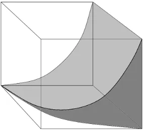
(22) Chapter 1 Introduction. 4. Figure 1.2: Bézier’s basic curve. independent beginnings, the foundations of modern CAD engines subsequently became largely established in the French car industry. It was in 1959 that Citroën hired a young mathematician, Paul de Faget de Casteljau, in order to resolve some of the theoretical problems that had arisen in the transition from the physical to computational representation of parts. Unlike Liming’s approach, de Casteljau initially built a system principally aimed at the ab initio design of curves and surfaces instead of concentrating on the computational duplication of their existing blueprints. From the start, he implemented the use of Bernstein polynomials with what is now known as the de Casteljau algorithm, and in doing so pioneered a new technique: control polygons (courbes à pôles). Instead of defining a curve (or surface) through points on it, a control polygon utilizes points near it. This meant that the curve (or surface) was not changed directly; instead, the alteration of the control polygon itself instigated an intuitive change in the curve (or surface). This work was kept secret by Citroën until the algorithm was first published by Krautter and Parizot (1971). Concurrently, Citroën’s competitor Renault had also realized the need for computational representations of mechanical parts. Renault’s design department was headed by Pierre Bézier who, although he was aware of similar developments at Citroën, proceeded to look at the theoretical problems of the transition independently. Using de Casteljau’s algorithm, Bézier’s initial idea was to characterize a “basic curve”, defined as the intersection of two elliptic cylinders; see Figure 1.2. These two cylinders were defined inside a parallelepiped, affine transformations of which would result in affine transformations of the curve. Later, polynomial formulations were developed and subsequently extended to higher degrees. It was not until the 1970s that there began a confluence of these different research.

(23) Chapter 1 Introduction. 5. approaches. In 1974, R. Barnhill and R. Riesenfeld used the construction and representation of free-form curves, surfaces or volumes to define a now very familiar term: Computer-Aided Geometrical Design or CAD. For further reading on the history of CAD, please refer to Farin (2002). Bézier’s work was widely published (Bézier, 1967, 1968, 1974, 1977) and Forrest’s article (Forrest, 1972) on Bézier curves contributed greatly to the popularity of Bézier curves. UNISURF, the Renault CAD/CAM system, was developed solely to use Bézier curves and surfaces. Dassault followed in Renault’s footsteps and built the system EVE, later evolving into CATIA (Computer Aided Three-Dimensional Interactive Application) (CATIA R , 2004). Today, CATIA, along with other commercial CAD packages, facilitates the use of both parametrically defined and “free-form” curves and surfaces. This ability to represent a design using an efficient mathematical model allows the CAD software to be coupled to an optimization process.. 1.1.2. The Role of Geometry Parameterization in CFD-Based Design Optimization. With the progress of CAD and CFD software, automated optimization processes using these computational tools have proven popular, allowing hi-tech industries to produce numerous computational designs quickly and relatively inexpensively. These designs can be analysed with respect to an appropriate measure of merit, evaluated and modified, and thus updated in a cyclical manner until a final optimal design is reached. Providing efficient design optimization processes has created a hub of activity within engineering research (Siddall, 1982). The enhanced efficiency of optimization techniques has enabled the search of larger design spaces in which optimal designs can be found in numerous varied applications; see Keane and Robinson (1999). Efficient optimization principally relies on concise sets of design parameters defining the geometry under examination. When a concise set of parameters is not readily available, designers may forego the potential to produce radical designs with a superior measure of merit. For previously tested and understood concepts and designs, design optimization is sometimes seen as a gradual evolution and improvement..

(24) Chapter 1 Introduction. 6. In cases where there is a limited understanding of the flow behaviour associated with the geometry under scrutiny, a reduced geometric control capability may prove detrimental in finding an optimal design. Ideally, the geometry parameterization would allow maximum control of the geometric shape whilst preserving a concise set of design parameters for the purpose of an efficient optimization process. However, the form of parameterization itself is often unclear. The literature on geometry parameterization techniques is substantial. Samareh (2001) surveyed a number of available techniques and assessed each on its suitability in dealing with complex models. It is clear that for design optimization studies, the particular geometry parameterization technique implemented can have an enormous impact on the final outcome. If a wing geometry is parameterized simply with planform and chord variation describing its shape, the optimal design may be localised to the area of the wing which these two particular features affect and so will not capture the true “global” nature of the wing shape that one may need to consider, including factors such as twist and sweep. A global geometry needs to be considered during a complete design process, and particularly in conceptual design. Local parameterization methods can be considered once a reasonably good global design has been reached, either through an initial optimization process or through a proven best pre-existing design. One of the first studies of an optimal condition with its analysis described by the mathematical theory of fluid dynamics was performed by Glowinski and Pironneau (1975). Subsequently, aerofoils became a popular subject for CFD-based optimization problems characterized by Hicks et al. (1974) and Jameson (1988). As a result of the extensive research performed on aerofoil and wing parameterization, it has become accepted to parameterize the overall shape of external wings through a set of well-known parameters: chord, span, planform, twist, sweep and shear. However, for internal fluid flow applications such as a diffuser, its parameterization cannot be defined using such well-known geometric quantities. In this case, manipulating the geometry to achieve a certain physical flow behaviour is a road less travelled. Diffusers have been the subject of optimization since the late 1950s. Early experimental work classified the major flow regimes within straight diffusers (Kline et al., 1959; Fox and Kline, 1962). Relationships were deduced between these flow regimes and the diffuser characteristics (Reneau, 1967) whilst, concurrently, simple geometry parameterizations gave room for more efficient designs; see Carlson et al. (1967). Although still.

(25) Chapter 1 Introduction. 7. experimental at this stage, this was an important start in recognizing the impact of geometry parameterization on the optimization process using analysis codes instead of practical experiments to determine results. In the last few decades, maximum optimizer efficiency for aerodynamic utilization has been sought, implying that a geometry parameterization containing a concise set of design variables is desirable. Madsen (1998), Madsen et al. (1999) and Madsen et al. (2000) have highlighted the use of geometry parameterization in optimization studies for straight diffusers and Ghate et al. (2004) parameterized an S-shaped duct for optimization. The development of parametric models within modern CAD engines is a key area of research. CAD, originally developed as an alternative to the drawing board, allowed for the improvement of design productivity and accuracy when first introduced. Common engineering shapes were soon parameterized and linked within the design part inside the CAD software to facilitate the automatic manipulation of the computational geometry to accommodate the required change. This eliminated the need for the designer to redraw the part in CAD and, in turn, made it practical to rapidly produce numerous design variations. The ability to differentiate between the large number of designs produced provided the link between CAD and analysis software such as CFD to optimize designs. CAD-based parameterization has distinct advantages over other approaches, as it enables large alterations from the original shape without necessarily destroying the shape topology. In addition, the less complex shape configuration does not require more advanced tools to enable mesh deformation in concurrence with shape change. Almost all engineering firms use CAD as an integral part of their design process. It is because of this that the scope of this thesis is limited to CAD-based parameterization techniques, aiming to offer a generic, practical and industrially realistic solution.. 1.2. Background and Objective of work. In this thesis, efficient and flexible methods of geometry parameterization are sought for use in an automated design optimization. Initially these are developed for use with a F1 airbox. This particular internal flow duct has been chosen due to the author’s interest in the sport and the lack of agreed practice in this particular industrial sector. After a thorough study of techniques used on plane geometries, the best and simplest.

(26) Chapter 1 Introduction. 8. parameterization for obtaining a good global shape is selected. Following this, a geometry manipulation technique is developed and used in a general automated design optimization process for a three-dimensional geometry. To illustrate the generic capability of the parameterization technique developed, a second case study has been tested: the shape optimization of a human carotid artery bifurcation. The choice of parameterization technique poses a similar problem but in this case the shape fit of the parametric model to that of a real artery geometry is optimized, aiming to achieve a close likeness. Early motoring was seen as a new and somewhat dangerous form of outdoor sport which presented a new element - the ever-changing machine - for the sportsman to contend with. Not only has the domestic car improved on a huge scale, the sport of motor-racing has developed alongside, the pinnacle of which for both drivers and manufacturers is the Formula One (F1) World Championship. The principles of aerodynamics developed from early aviation have been passed into the automotive industry and used to enhance the performance of racing cars. With the advent of the F1 World Championship, chassis design, engine technology, suspension technology and aerodynamic aids improved. F1 cars became faster, more agile and more spectacular to watch. The rapid development of computational power has permitted the feasibility of computational design, and latterly, shape optimization. The design of engine air intakes, in particular those used in F1, has become a significant consideration as engines continually improve in sophistication and performance. Intake design seeks to maximize static pressure acting on the intake stroke of the engine cylinders. High static pressure over the cylinders increases the cylinder charge density and hence engine power. The design of the airbox geometry, including its bend through 90◦ and the position of the air filter element, all have an impact on both the static pressure recovery and cylinder-to-cylinder air distribution and thus engine performance. During the first few decades of the 20th century, it was known that diffusers could convert kinetic energy at the diffuser entry into static pressure at the exit, albeit with low efficiency. Improvement of the efficiency of this effect started in 1938 (Patterson, 1938). F1 aerodynamicists have studied engine air intakes since the 1950s. These began as small air vents in the engine cover bodywork over the cylinders in front of the driver. Ten years.

(27) Chapter 1 Introduction. 9. Figure 1.3: Airbox inlet (2003 season). later, the introduction of rear-engined cars left the engines exposed with no covering bodywork. By 1972, the teams had designed large scoop-like airboxes sitting above the driver’s head. Safety, however, increasingly became an issue and roll bar structures were introduced. Two large scoops either side of the roll bar then became the norm, reducing in size through the early eighties until, in 1989, airboxes appeared akin to those seen today, see Figure 1.3. F1 is a highly competitive sport and so time, cost and good results are critical. Careful design of individual components can often provide the necessary advantage to enhance performance. However, regulation constraints may limit the level of design improvement. For modern air intakes, expansion of the flow is required over a short distance while turning through 90◦ due to the roll bar specifications and engine layout configuration; see FIA (2005). During the time of the present study, the F1 teams place a 3-litre V10 engine behind the driver (see Figure 1.4); the position of the airbox thus takes advantage of the ramming effects of the oncoming air at high speeds. The engine filter is located over a trumpet tray, at the bottom of which sits an offset array of 10 engine inlet trumpets, one for each of the cylinders. For the 2006 season, the engine specification has changed to 2.4-litre V8 engines. The airboxes are very similar in their positioning to the illustration in Figure 1.4, the only difference between the airboxes contained in this thesis and the ones that will be seen on the track in 2006 is the number of cylinders: 10 instead of 8. Interestingly, during the pre-2006 season testing when the V8 engines were not yet ready for the track, the cars were seen with an airbox inlet adaption, illustrated in Figure 1.5. By limiting the.

(28) Chapter 1 Introduction. 10 airbox. airbox inlet. roll bar air filter (airbox exit). ENGINE Figure 1.4: Airbox positioning within the F1 car. Figure 1.5: Restriction of entry area to limit engine power (see inset), seen to have been used on certain F1 cars during the pre-2006 season testing. air to the engine, the performance was reduced sufficiently to simulate the performance that would be experienced from the new, less powerful, engine. In comparison to race car design, arterial geometry parameterization is a relatively new topic of research. However, the use of computational modelling has become a powerful research tool in aiding the understanding of arterial biomechanical behaviour and its relation to atherosclerosis, a common disease which can lead to stroke, heart attacks, eye and kidney problems. A detailed and informative review of computational techniques currently being used for research into patient-specific biomechanics for potential treatment decision making can be found in Steinman et al. (2003). Although surgeons have not yet accepted these techniques for routine clinical use, an improved understanding of local haemodynamics in a broad variety of different conditions, including the effect after surgical intervention, may lead ultimately to the possibility of a patient-specific.

(29) Chapter 1 Introduction. 11. predictive medicine approach to surgical intervention. Taylor et al. (1999) has adopted this approach for the planning of bypass surgery, Guadagni et al. (2001) discusses optimizing the treatment of congenital heart defects and Cebral et al. (2000) and Steinman et al. (2002a) uses the approach for cerebral aneurysms. It is widely accepted that internal wall geometry is correlated with the sites of atherosclerosis. Early experimental and CAD models of the carotid artery bifurcation were highly idealised as “Y-shaped” models. Although better approximations are now used through “tuning fork” artery shapes, they can be applied only in a general sense. Examples of a Y-shaped artery model and a tuning fork artery model in comparison with the shape of a real artery model can be seen in Figure 1.6. Much more sophisticated image processing techniques have been developed for 3D geometry reconstruction of arteries based on Magnetic Resonance Imaging (MRI) (Steinman, 2002; Steinman et al., 2002b; Antiga and Steinman, 2004). This method captures the large variation in shape and dimensions of the arteries from patient to patient. For patient specific analysis it is important to capture an accurate computational representation of the artery for accurate flow simulations. Through accurate CFD modelling in realistic arteries, doctors are beginning to understand the link between the arterial haemodynamics, other physiology and the build up of disease. However, parametric models are also of importance to develop an understanding of how changes in arterial wall shape affect the haemodynamic behaviour. The industry, at present, although possessing powerful visualization tools to represent and reconstruct extremely accurate computational arteries, lacks a realistic parametric model for use in computational research. One key benefit of a realistic parametric geometry is to enable research to determine those patients for whom interventional medicine may be favourable. For example, by understanding the haemodynamics connected with key geometrical factors, a connection between arterial geometry and a pre-disposition of lower leg iscaemia in certain diabetics may be discovered. The techniques developed for studying F1 airboxes have been adopted here for building arterial models. The main objective of this thesis is to develop a fully automated general-purpose parameterization strategy providing a global manipulation of the geometry surface followed by a local surface deformation for use in the design optimization of three-dimensional internal fluid flow applications..

(30) Chapter 1 Introduction. 12. Figure 1.6: Y-shaped artery model (left), tuning fork artery model (centre) and real artery model (right). 1.3. Thesis Outline. In Chapter 2, the setup of an automated design optimization process is discussed. Each part of the process is described in detail and the geometry parameterization techniques available in commercial CAD software packages are surveyed. The implementation of a Design of Experiments (DoE) approach followed by the use of CFD is described and response surface methodology is proposed as the optimization approach used in this thesis. Response surface methodology is a means of quickening an exhaustive search process to find an optimal design. Chapter 3 contains a mathematical description, in general terms, of response surface approximation theory. Kriging is the focus here, and a discussion of the various search techniques is given. Furthermore, for computationally expensive cases, a concentrated exploration in a reduced area of the response surface for additional improvement in design and convergence towards an optimum is described. Chapter 4 implements a number of techniques surveyed in Chapter 2 in the design optimization of a plane straight expanding duct and a constant width elbow turning through 90◦ . The results of these studies are compared and each technique is analysed with respect to the number of design variables required and the amount of global shape control given. As the straight diffuser and elbow comprise both the features of an airbox in terms of expansion and turning of the flow, a suitable parameterization technique with good global shape control for a plane F1 airbox is then proposed and implemented in a 2D design optimization study..

(31) Chapter 1 Introduction. 13. The purpose of Chapter 5 is to propose a general automated multi-stage design optimization process for three-dimensional internal fluid flow applications with the capability of providing both a globally parametric representation of the geometry as well as a locally adaptable representation. The first stage is a global technique allowing the identification of a generally good geometry, and the second stage is a local technique providing features unavailable with the global technique for fine-tuning the geometry to gain improvements towards an optimal design representation. This chapter presents a survey of 3D surface representations, and from the conclusions drawn, the most appropriate surface manipulation techniques are chosen and a general automated process outlined. In Chapter 6, the automated multi-stage optimization process built up in previous chapters is applied to a three-dimensional F1 airbox. A parametric geometry is constructed and a good global geometry found. The second stage of the process is implemented and local deformations of the airbox surface are optimized to achieve a high performance geometry. Chapter 7 considers the multi-stage optimization process developed in Chapter 5, but now applied to the shape optimization of a realistic parametric human carotid artery bifurcation model. The initial artery geometry is determined from an automated analysis of scanned data of a real artery. The error between the parametric CAD model and the real artery is minimized through a local geometry manipulation stage. CFD analysis is performed on the resulting CAD model and compared with a CFD simulation through the ‘real’ artery. Finally, in Chapter 8, the contributions made are noted and general conclusions drawn from the work presented along with suggestions for future research resulting from these investigations..

(32) Chapter 2. Design Optimization Methodology Optimization, in short, can be described as the action or process of rendering the most favourable outcome under a particular set of circumstances. Optimization as a concept is familiar to all as, instinctively, we search for the best solution given a set of circumstances in many everyday activities. This general concept of optimization is ubiquitous in countless applications, for example, in engineering design, biomechanics, weather prediction, econometrics and financial forecasting to name but a few. In formulating a design optimization problem, we wish to find the best solution to a specific problem defined by a finite number of design variables, such that a desired performance criterion can be maximized (e.g. recovery time, fuel efficiency, profit, etc.) or minimized (e.g. aerodynamic drag, weight, loss, etc.). This criterion can be expressed explicitly in terms of an ‘objective function’. In addition to this, limitations or ‘constraints’ may be imposed (e.g. physical size, manufacturing capability, economic). By systematically adjusting the values of all design variables, a ‘good’ (feasible) or ‘best’ (optimal) solution may be found. In mechanical design an optimization framework commonly incorporates geometry construction, analysis and post-processing software, each of which has developed throughout the course of the last 40 years, often independently. As a result, difficulties often arise in determining an optimal solution when an efficient automation of the process cannot 14.

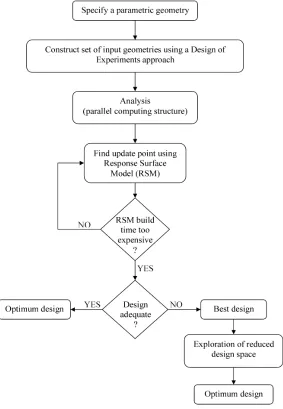
(33) Chapter 2 Design Optimization Methodology. 15. Figure 2.1: A generalised optimization strategy. be achieved due to software incompatibility. In an optimization process one must accept possible limitations generated from software integration difficulties. A typical design optimization framework is illustrated in Figure 2.1, each step of which is discussed in further detail in the subsequent sections, giving a description of the automated system architecture employed throughout this thesis..

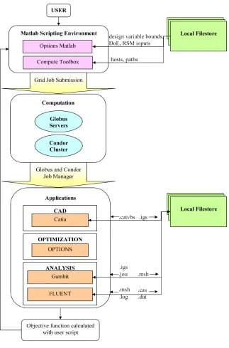
(34) Chapter 2 Design Optimization Methodology. 2.1. 16. An Automated System Architecture. One of the primary issues faced by industries employing various software technologies is that of the incompatibility between the software input and output file requirements. To circumnavigate these issues, in-house codes may be written largely to provide a seamless integration of software. However, due to the nature of industry, these codes are rarely homogeneously shared across all business units resulting in wasted effort, time and money as different units produce their own ad hoc solutions. To remain consistent with the use of only commercially available design and analysis software in this thesis, the design optimization process is incorporated within the GridEnabled Optimization and Design Search for Engineering (GEODISE) system (Geodise, 2002). The GEODISE system is implemented using the Matlab lab. R,. R. environment (Mat-. 2002) as an engineering portal giving remote access to the required CAD software. CATIA V5. R. Dassault Systèmes, analysis software FluentTM (2003a) and optimization. software OPTIONS (Keane, 2002). Matlab is adopted due to its prevalence in the engineering fraternity, making the toolkit flexible and easily extendible. As the use of optimization in design is becoming more commonplace, and designers are demanding evermore accurate simulations, larger models are being tested requiring CFD computations many orders of magnitude larger than the optimization methods themselves. This in turn requires greater computational resources making this process well suited to the use of Grid computing (Foster, 2002; Eres et al., 2005). For many designers the integration of several heterogeneous environments and/or incompatible software on such a large scale would be a daunting undertaking. The development of Grid technologies with the Open Grid Services Architecture (OGSA) (Foster et al., 2002) and the Open Grid Services Infrastructure (OGSI, 2003) has allowed this type of service-orientated computation to become easily adopted. The GEODISE toolkit is composed of a hierarchy of components which is depicted in Figure 2.2. Each box, from the scripting environment through computation to the applications, are exposed as Grid services and are connected appropriately in this service-based workflow; see Xue et al. (2004). Low level compute toolbox functions are available along with the input scripts for the OptionsMatlab toolbox. Users can then access remote compute resources such as the Condor Cluster shown in Figure 2.2, where the Globus.

(35) Chapter 2 Design Optimization Methodology. 17. Figure 2.2: GEODISE system architecture. server (Globus, 2002) provides the middleware allowing the compilation of the remote resources. This server provides much of the functionality that the system requires including authentication, authorization, job submission, data transfer and resource monitoring. The applications box depicted in Figure 2.2 holds the array of higher level geometry, optimization, pre- and post-processing and CFD functions that the toolkit then calls with the appropriate input files from the user’s filestore..

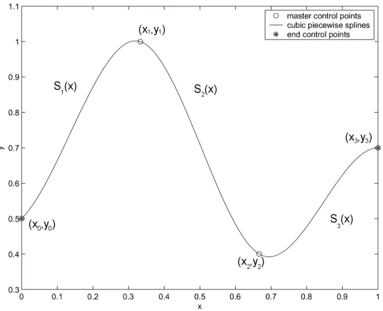
(36) Chapter 2 Design Optimization Methodology. 2.2. 18. Geometric Parameterization. To begin the design search and optimization process shown in Figure 2.1, a parametric geometry must first be considered. Parameterization is here defined as the specification of a geometry by means of a finite number of parameters or design variables which are allowed to assume values in a given bounded range. The choice of method for geometric parameterization becomes crucial when used in conjunction with an optimizer. This choice is problematic, however, as in many situations one is faced with myriad feasible methods, sometimes with no real distinction between the advantages of one over another. The challenge is in selecting an appropriate set of design variables to allow a large amount of geometric variability or ‘strong shape control’ of the CAD created geometry, whilst retaining as compact a set as possible for the sake of efficient optimization. Strong shape control is important, allowing the optimizer to discover less intuitive designs with the potential to produce superior results. A proper choice of design variables usually requires a good understanding of the flow physics surrounding the geometry and the type of design variables likely to affect the objective function. In many internal fluid flow applications, however, the flow behaviour is not clearly understood. In particular, for cases where the designer is unable to predict likely changes in flow behaviour caused by certain changes in the geometry and whether these changes are likely to improve the design. In the absence of a clear understanding of the flow physics, strong shape control is essential in order to relate the design variables to the flow behaviour . A survey of the most common curve parameterization methods has been performed to determine the best choice of method to achieve strong shape control, retaining a set of only few design variables.. 2.2.1. Polynomial Curves. In the field of numerical analysis, a spline is regarded as a special function defined in a piecewise manner by polynomials. In computer science, in particular the subfields of CAD and computer graphics, a spline is regarded as a piecewise parametric polynomial curve (Farin, 1990). Spline approaches to curve contouring have the advantages of providing a compact set of design variables and are naturally smooth. It is a popular representation, not only due to its inherent smoothness but also due to the simplicity of.

(37) Chapter 2 Design Optimization Methodology. 19. Figure 2.3: A piecewise cubic spline. its construction and evaluation and its capacity to create complex shapes. An example of a spline parameterization can be seen in Figure 2.3. Here, a piecewise spline comprising three polynomial (cubic) curves S1 (x), S2 (x) and S3 (x) with end control points at (x0 ,y0 ) and (x3 ,y3 ) and two mid master points (x1 ,y1 ) and (x2 ,y2 ) is shown. At each of the mid master points, the piecewise splines join with first and second order continuity. In its most general form, a univariate polynomial spline S : [a, b] → R consists of polynomial pieces Si : [xi , xi+1 ] → R, where. a = x0 < x1 < · · · < xn−1 < xn = b.. (2.1). Hence,. S(x) = S1 (x),. x0 ≤ x < x1 ,. S(x) = S2 (x),. x1 ≤ x < x2 ,. .. . S(x) = Sn (x),. (2.2). xn−1 ≤ x < xn .. The vector x = (x0 , x1 , ..., xn ) is known as the knot vector and if the knots are equidistant it is a uniform spline. The smoothness is determined by the parametric continuity of.

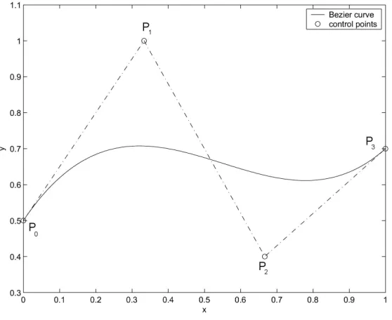
(38) Chapter 2 Design Optimization Methodology. 20. one polynomial piece to the next. Continuity C j implies that the two adjoining pieces Si and Si+1 share common derivative values from order zero to order j. The advantages of using this technique are the ease with which one can define parametric continuity, specify the curve tangency at the start and end of the curve and have interpolation through all the control points given. However, in cases where C 2 is imposed, one may see a tendency for the curve to oscillate. If this occurs, small changes could lead to dire ramifications on the geometry. By changing only one control point position, the entire curve is modified which would not be ideal if only a local change to the curve is desired. If a complex shape is modelled, the degree may be increased to allow for greater flexibility, however, this would incur a greater computational effort to evaluate the curve with a large number of points needed to describe the complex shape. For the remainder of this thesis, the focus is mainly on the cubic spline, where each Si is of degree 3, and the term “spline” in used in this restricted sense.. 2.2.2. Bézier Curves. For simple geometries, Bézier curves (Bézier, 1970) are equally as effective as polynomial splines with, again, smooth and accurate properties represented concisely. Braibant and Fleury (1984) demonstrated that Bézier curves are well suited to geometric parameterization when used in optimization studies, while Farin (1990) describes some of the more useful properties of this particular technique. In essence, a Bézier curve approximates a set of points, as opposed to the interpolation seen with polynomial splines, although the curve end points are interpolated. A Bézier curve can be calculated based on some n + 1 points to be interpolated. An example of a Bézier curve parameterization can be seen in Figure 2.4 with two master control points P0 and P3 , through which the curve interpolates, and two knots P1 and P2 four control points in total. Using this method one cannot prescribe the start and end tangency conditions. This is determined by the tangency calculated between the first two control points (P0 , P1 ) and the last two control points (P2 , P3 ) respectively. An additional advantage of this technique is that it is useful for curve collision detection, as the curve will lie within the convex closure of the control points. A Bézier curve is.

(39) Chapter 2 Design Optimization Methodology. 21. Figure 2.4: A Bézier curve. also invariant under affine transformations, i.e., rotation, scaling or translation of the control points result in the rotation, scaling or translation of the curve itself. Mathematically, a Bézier curve can be defined as follows. Given a set of n + 1 control points P0 , . . . , Pn , the Bézier (or Bernstein-Bézier) curve is given by. S(x) =. n X. Pi bi,n (x). (2.3). i=0. where the Bernstein polynomial bi,n is defined as. . bi,n = . n i. .  xi (1 − x)n−i. (2.4). where x ∈ [0, 1] and i=0,...,n. Similar to the polynomial splines, these curves do not offer strong shape control, nor do they offer an efficient way of describing complex shapes where a large number of control points are required or where a high order curve is needed. One way of improving this efficiency would be to divide the single Bézier curve into a number of lower order Bézier curves but this has its own disadvantage in that it becomes more difficult to ensure smoothness at the curve joins..

(40) Chapter 2 Design Optimization Methodology. 2.2.3. 22. B-splines. B-splines refers to basis splines. Their useage as parametric curves was investigated by Schoenberg in the 1940s but did not become popular until the publications by de Boor and Cox in the 1970s (de Boor, 1972; Cox, 1972) where they discovered recurrence relations facilitating rapid evaluation of the basis functions. A generalized B-spline is defined as follows. Suppose that we have a knot vector x containing m + 1 knots x0 ≤ x1 ≤ ... ≤ xm , a B-spline is given by:. S(x) =. m X. Pi αi,n (x). i=0. x ∈ [x0 , xm ],. (2.5). where Pi are the control points and αi,n (x) are the basis functions. The m by n B-spline basis functions of degree n can be defined using the Cox-de Boor recursion formula,. αj,0. αj,n (x) =.   1 =  0. if xj ≤ x < xj+1 otherwise. x − xj xj+n+1 − xj αj,n+1 (x) + αj+n,n−1 (x). xj+n − xj xj+n+1 − xj+1. (2.6). If the knots are equidistant then the B-spline is considered uniform. If n = m then the B-spline degenerates into a Bézier curve. A B-spline has strong shape control and has all the advantages of the Bézier curves although it is stricter in the sense that a B-spline will lie within the union of the convex closures of all segments and also provides greater shape control as moving a control point does not affect the whole curve, unlike polynomial curves.. 2.2.4. Hicks-Henne Bump Functions. Hicks and Henne (1978) developed a global shape function to efficiently modify aerofoil sections. These are analytical shape functions which allow for strong shape control and can be written in a general form (see Sóbester and Keane (2002)):.

No results found