Rochester Institute of Technology
RIT Scholar Works
Theses Thesis/Dissertation Collections
1-2015
Performance and Energy Trade-offs for 3D IC
NoC Interconnects and Architectures
James David Coddington
Follow this and additional works at:http://scholarworks.rit.edu/theses
This Thesis is brought to you for free and open access by the Thesis/Dissertation Collections at RIT Scholar Works. It has been accepted for inclusion in Theses by an authorized administrator of RIT Scholar Works. For more information, please [email protected].
Recommended Citation
Performance and Energy Trade-offs for 3D IC NoC
Interconnects and Architectures
by
James David Coddington
A Thesis Submitted in Partial Fulfillment of the Requirements for the Degree of Master of Science in Computer Engineering
Supervised by
Dr. Amlan Ganguly
Department of Computer Engineering Kate Gleason College of Engineering
Rochester Institute of Technology Rochester, NY
January, 2015
Approved By:
_____________________________________________ ___________ ___
Dr. Amlan Ganguly
Primary Advisor – R.I.T. Dept. of Computer Engineering
_ __ ___________________________________ _________ _____
Dr. Andres Kwasinski
Secondary Advisor – R.I.T. Dept. of Computer Engineering
_____________________________________________ ______________
Dr. Juan Cockburn
Dedication
I would like to dedicate this thesis to my wife Gwenlyn and my parents Dave and Kim
Coddington. They have been consistently supporting me throughout my academic career
Acknowledgements
I’d like to thank my advisor, Dr. Amlan Ganguly for his expertise and help throughout
my graduate research. I’d also like to thank my committee members Dr. Juan Cockburn
and Dr. Andres Kwasinski for their constructive feedback and professional opinions.
Lastly, I’d like to thank Shahriar Shamim for his help getting started with the
Abstract
With the increased complexity and continual scaling of integrated circuit
performance, multi-core chips with dozens, hundreds, even thousands of parallel
computing units require high performance interconnects to maximize data throughput and
minimize latency and energy consumption. High core counts render bus based
interconnects inefficient and lackluster in performance. Networks-on-Chip were
introduced to simplify the interconnect design process and maintain a more scalable
interconnection architecture. With the continual scaling of feature sizes for smaller and
smaller transistors, the global interconnections of planar integrated circuits are
consuming higher energy proportional to the rest of the chip power dissipation as well as
increasing communication delays. Three-dimensional integrated circuits were introduced
to shorten global wire lengths and increase chip connectivity. These 3D ICs bring heat
dissipation challenges as the power density increases drastically for each additional chip
layer. One of the most popularly researched vertical interconnection technologies is
through-silicon vias (TSVs). TSVs require additional manufacturing steps to build but
generally have low energy dissipation and good performance. Alternative wireless
technologies such as capacitive or inductive coupling do not require additional
manufacturing steps and also provide the option of having a liquid cooling layer between
planar chips. They are typically much slower and consume more energy than their wired
counterparts, however. This work compares the interconnection technologies across
several different NoC architectures including a proposed sparse 3D mesh for inductive
Table of Contents
Dedication ... ii
Acknowledgements ... iii
Abstract ... iv
Table of Contents ... v
List of Figures ... viii
List of Tables ... xi
Chapter 1 Introduction ... 1
1.1. From Single to Multi-Processor Systems ... 1
1.2. Network-on-Chip Data Routing ... 2
1.3. To The Third Dimension ... 3
1.4. Thesis Contributions ... 4
Chapter 2 Related Work ... 6
2.1. 3D ICs ... 6
2.2. 3D Wired NoCs ... 6
2.3. 3D Wireless NoCs ... 7
2.4. Emerging Technologies ... 7
Chapter 3 Wired 3D NoC Architectures ... 9
3.1. Dense 3D Mesh NoC ... 9
3.3. NoC Performance Evaluation ... 11
3.3.1 Bandwidth ... 12
3.3.2 Energy per Message ... 13
3.3.3 Network Latency ... 14
3.4. NoC Performance Evaluation with Non-Uniform Traffic ... 15
3.4.1 Energy per Message ... 15
3.4.2 Network Latency ... 17
3.5. TSV Density Analysis ... 17
3.5.1 NoC Performance Evaluation... 18
3.5.2 NoC Performance Evaluation with Non-Uniform Traffic ... 23
3.6. Area Overheads ... 27
Chapter 4 Wireless 3D NoC Architectures ... 28
4.1. Performance Evaluation ... 30
4.1.1 Bandwidth ... 30
4.1.2 Energy per Message ... 32
4.1.3 Latency ... 35
4.2. Performance Evaluation with Non-Uniform Traffic ... 36
4.2.1 Energy per Message ... 37
4.2.2 Latency ... 39
Chapter 5 Conclusions ... 42
5.1. Summary ... 42
5.1.1 System Bandwidth... 42
5.1.2 System Energy per Message ... 43
5.1.3 System Latency ... 46
5.1.4 Chip Area ... 49
5.1.5 Overall ... 50
5.2. Future Work ... 50
List of Figures
Figure 1-1: 16 Core 2D Mesh Network-on-Chip ... 2
Figure 3-1: One Plane of a Dense 3D Mesh ... 9
Figure 3-2: 3D Connections for a Dense 3D Mesh ... 9
Figure 3-3: TSV Uniform Traffic Peak Bandwidth ... 12
Figure 3-4: TSV Uniform Traffic Energy per Message... 13
Figure 3-5: TSV Uniform Traffic Energy per Message without Waiting ... 14
Figure 3-6: TSV Uniform Traffic Average Latency ... 15
Figure 3-7: TSV Non-Uniform Traffic Energy per Message ... 16
Figure 3-8: TSV Non-Uniform Traffic Energy per Message without Waiting .... 16
Figure 3-9: TSV Non-Uniform Traffic Average Latency... 17
Figure 3-10: TSV Density Analysis with 32 bits/flit Uniform Traffic Peak Bandwidth ... 19
Figure 3-11: TSV Density Analysis with 64 bits/flit Uniform Traffic Peak Bandwidth ... 19
Figure 3-12: TSV Density Analysis with an 8x4x8 NoC and 32 bits/flit Uniform Traffic ... 20
Figure 3-13: TSV Density Analysis with an 8x8x8 NoC and 32 bits/flit Uniform Traffic ... 20
Figure 3-14: TSV Density Analysis with 32 bits/flit Uniform Traffic Energy per Message... 21
Figure 3-16: TSV Density Analysis with 32 bits/flit Uniform Traffic Energy per
Message without Waiting ... 22
Figure 3-17: TSV Density Analysis with 64 bits/flit Uniform Traffic Energy per
Message without Waiting ... 22
Figure 3-18: TSV Density Analysis with 32 bits/flit Uniform Traffic Average
Latency ... 23
Figure 3-19: TSV Density Analysis with 64 bits/flit Uniform Traffic Average
Latency ... 23
Figure 3-20: TSV Density Analysis with 32 bits/flit Non-Uniform Traffic Energy
per Message ... 24
Figure 3-21: TSV Density Analysis with 64 bits/flit Non-Uniform Traffic Energy
per Message ... 24
Figure 3-22: TSV Density Analysis with 32 bits/flit Non-Uniform Traffic Energy
per Message without Waiting ... 25
Figure 3-23: TSV Density Analysis with 64 bits/flit Non-Uniform Traffic Energy
per Message without Waiting ... 25
Figure 3-24: TSV Density Analysis with 32 bits/flit Non-Uniform Traffic
Average Latency ... 26
Figure 3-25: TSV Density Analysis with 64 bits/flit Non-Uniform Traffic
Average Latency ... 26
Figure 4-1: 3D Ring NoC ... 29
Figure 4-3: Wireless Comparison with 32 bits/flit Uniform Traffic Peak
Bandwidth ... 31
Figure 4-4: Wireless Comparison with 64 bits/flit Uniform Traffic Peak
Bandwidth ... 31
Figure 4-5: Wireless Comparison with 32 bits/flit Uniform Traffic Energy per
Message... 33
Figure 4-6: Wireless Comparison with 64 bits/flit Uniform Traffic Energy per
Message... 34
Figure 4-7: Wireless Comparison with 32 bits/flit Uniform Traffic Energy per
Message without Waiting ... 35
Figure 4-8: Wireless Comparison with 64 bits/flit Uniform Traffic Energy per
Message without Waiting ... 35
Figure 4-9: Wireless Comparison with 32 bits/flit Uniform Traffic Average
Latency ... 36
Figure 4-10: Wireless Comparison with 64 bits/flit Uniform Traffic Average
Latency ... 36
Figure 4-11: Wireless Comparison with 32 bits/flit Non-Uniform Traffic Energy
per Message ... 37
Figure 4-12: Wireless Comparison with 64 bits/flit Non-Uniform Traffic Energy
per Message ... 38
Figure 4-13: Wireless Comparison with 32 bits/flit Non-Uniform Traffic Energy
Figure 4-14: Wireless Comparison with 64 bits/flit Non-Uniform Traffic Energy
per Message without Waiting ... 39
Figure 4-15: Wireless Comparison with 32 bits/flit Non-Uniform Traffic Average
Latency ... 40
Figure 4-16: Wireless Comparison with 64 bits/flit Non-Uniform Traffic Average
Latency ... 40
List of Tables
Table 4-1: Technology and Architecture Pairs System Average Hop Count
Comparison ... 31
Table 4-2: Technology and Architecture Pairs 32 bits/flit System Bandwidth
Comparison ... 32
Table 4-3: Technology and Architecture Pairs 64 bits/flit System Bandwidth
Comparison ... 32
Table 4-4: Technology and Architecture Pairs System Chip Area Overhead
Chapter 1
Introduction
In recent years, the technological advancements in the production of large scale
integrated circuits have been accelerating at a rapid pace and because of this, chip
designers are getting closer and closer to regularly utilizing tens of billions of transistors
on a single chip. Engineers are pressed with designing ever more efficient and powerful
processors to perform tasks for fields that range from consumer level electronics devices
to supercomputing workloads such as astrophysics, pollution and weather forecasting and
modeling, fluid dynamics, and bioinformatics.
1.1. From Single to Multi-Processor Systems
For a considerable period of time in the electronics industry, it was sufficient to
simply increase the operating frequency to get a considerable increase in performance.
Recently, however, clock speed increases have slowed substantially due to high power
dissipation from the increased switching activity density of the transistors. It is becoming
increasingly difficult to remove all of the excess heat from the chip. This power restraint
has shifted the design paradigm from single core processors to multicore processors and
has unleashed several new challenges for chip designers [1]. Multicore processors
enabled designers to utilize the additional transistors to increase performance with the
addition of core-level parallelism.
One of the most difficult challenges for multi-processor systems is how to connect
the individual cores to each other without limiting the performance. Some of the first
multicore processors utilized a shared bus for communication between the cores. As the
have come to establish themselves as a limiting factor in the performance of a system [2].
In response, systems have been moving from shared-bus based architectures with longer
wires to scalable Network-on-Chip (NoC) architectures with shorter wires to handle the
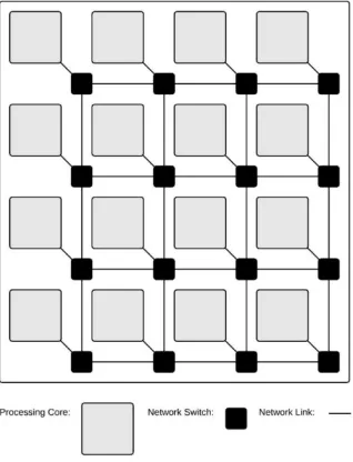
increased communication demands for many-core chips [3]. An example 16 core 2D
mesh NoC is shown in Figure 1-1. This figure shows how packets must go through at
least six hops to go from one corner of the chip to the opposite corner. As more and more
cores are added to the system, communication performance for data traveling from one
end of the chip to the other degrades due to the increased number of cycles it takes for a
packet to move through the network to its destination, even with a scalable NoC.
[image:14.612.227.386.329.537.2]
Figure 1-1: 16 Core 2D Mesh Network-on-Chip
1.2. Network-on-Chip Data Routing
For routing data between cores in a NoC, there are conventionally three options:
circuit switching, packet switching, and wormhole routing. Circuit switching reserves a
path from the sending node to the receiving node to send the data. This prevents other
Packet switching breaks the data into packets where each packet is sent over the network
separately. This requires the entire packet to be buffered at each intermediate node and
takes considerable chip area to implement. One of the more popular routing schemes for
NoCs is wormhole routing where a data packet that needs to be transferred from one part
of the chip to another is broken into smaller flow control units called flits. The header flit
contains all of the routing information and is sent first, reserving the path for the rest of
the flits to follow [3]. Similar to circuit switching, wormhole routing reserves paths such
that multiple packets cannot be sent through a single switch at the same time. To get
passed this, virtual channels separate the packets so that more of the network capacity can
be utilized. Wormhole routing is more commonly used in systems where chip area
overheads are important and is utilized in this work.
1.3. To The Third Dimension
As the chip dimensions and number of cores continue to grow, the global
interconnect wires continue to get longer and their relative performance degrades
compared to the speed increases of transistors. In an effort to reduce the number of clock
cycles it takes for packets to traverse the NoC and get further performance increases, 3D
integrated circuits (3D ICs) have emerged as a viable method of shrinking the
communication distances and allowing the NoC to have a higher connectivity [4]. The
shorter distances and higher connectivity both contribute to higher performance.
Although the overall wire lengths are reduced by switching to 3D ICs, the power density
is increased significantly. The number of transistors per square millimeter increases
substantially with each IC layer. This leads to higher heat dissipation, which needs to be
network topology play an important role in the NoC performance and energy
consumption and need to be evaluated. Several technologies have evolved into viable
solutions for transferring data between the layers in the 3D ICs including Through Silicon
Vias (TSVs), capacitive coupling circuits, and inductive coupling circuits. Each
technology has its own distinct advantages and disadvantages which will be explored in
more detail in 0 and 0.
1.4. Thesis Contributions
In this work, a comparative analysis of several vertical interconnect technologies
and 3D-NoC architectures is performed. This includes a comparison of TSV, inductive
coupling, and capacitive coupling based vertical interconnects in addition to the impact
that TSV density has on network performance and energy consumption. It also includes a
comparison of inductive coupling dense 3D mesh and ring networks to a proposed novel
sparse 3D mesh architecture. This architecture is designed to reduce chip area overhead,
latency, and the energy per message while minimizing the impact to the overall
throughput of the network. To accomplish this, the delay and power of vertical
interconnections for TSV, inductive coupling, and capacitive coupling technologies are
modeled, a novel inductive coupling 3D-NoC architecture is proposed, and a 3D-NoC
cycle accurate simulator is developed. The simulator is used to run simulations with
various types of network traffics and benchmarks to be able to compare the different
technologies and network architectures. Simulation parameters including core count,
packet size, and network traffic patterns will be varied to find differences in the energy
dissipation per message, the bandwidth of the system, and the average latency of the
• Delay and Power Modeling
• TSV Delay and Power Modeling for Various TSV Densities
• Inductive Coupling Delay and Power Modeling
• Capacitive Coupling Delay and Power Modeling
• Architecture Comparisons
• TSV Dense 3D Mesh
• Inductive Coupling Dense 3D Mesh
• Inductive Coupling Two-Way Ring
• Inductive Coupling Sparse Mesh
• Capacitive Coupling Dense Mesh
• Simulator Framework
• Cycle Accurate Simulator for 3D NoCs with 3-Stage Switches
• Input Arbitration
• Output Arbitration
• Routing
• Experimental Results for the Various 3D Technologies and Architectures
• Peak Bandwidth
• Energy Dissipated Per Message
• Latency
• Non-Uniform and Uniform Traffic Patterns
• Scalability with Respect to Increasing Message Size and Core
Chapter 2
Related Work
2.1. 3D ICs
The problems associated with the high wiring connectivity requirements of
large-scale integration circuit design is explored in [5] along with how 3D ICs increase
connectivity while reducing the number of long interconnects. Similarly, the authors of
[6] and [7] investigate how 3D ICs can be used to combat the growing ratio of
interconnect to gate delay as feature sizes decrease. A general overview of 3D
technologies and the motivations behind designing 3D integrated circuits is presented in
[8]. The benefits of using a 3D NoC instead of a 2D NoC are explored by Feero and
Pande [4]. Their work focused on the performance and area effects of the network
architectures rather than the power and performance tradeoffs of various technologies.
The effects of serialization and a general comparison between TSV, inductive coupling,
and capacitive coupling are discussed in [9]. However, the authors did not investigate
power consumption and the effects of the vertical connection topologies. Chip
manufacturers have their choice of network architectures and vertical interconnect
technologies where the impact of power, performance, and chip area overheads are
important.
2.2. 3D Wired NoCs
As one of the more popular vertical connection technologies, through silicon vias
(TSVs) and some of their manufacturing techniques are explained in [10] along with TSV
manufacturing process for 3D ICs but they tend to offer good power, performance, and
chip area characteristics.
2.3. 3D Wireless NoCs
In [11], a low power and high data rate inductive coupling transceiver is
proposed. Inductive coupling is a vertical connection technology that does not require
modifications to the manufacturing process, but the power, performance, and chip area
overheads are often prohibitive to the adoption of the technology. The design and
implementation of a capacitive coupling transceiver is analyzed in [12] where the power,
performance, and area overheads are discussed as well as restrictions that capacitive
coupling links put on how the layers of the 3D ICs are assembled. Capacitive coupling
also does not require changes to the manufacturing process but limits vertical scaling to
two layers placed faced to face instead of multiple layers placed face to back. It also
exhibits poor power, performance, and chip area overheads relative to inductive coupling
and wired techniques.
2.4. Emerging Technologies
Some experimental technologies show potential for being effective at reducing
energy consumption and increasing performance but are not covered in this work. One of
the more promising technologies is photonic interconnects. Photonic interconnects
transfer data by sending signals over optical waveguides. In [13], TSVs and a
reconfigurable photonic network are utilized to reduce energy consumption while
maintaining performance. Photonic interconnects have the benefit of their bandwidth
manufacturing steps that are required to build circuits that include photonic interconnects.
These extra steps add to the complexity and overall cost of these systems.
Another technology for connecting cores in a system utilizes wireless
interconnects. Radio frequency transceivers can be built into the chip and used to transmit
data across larger distances with less power and less latency than traditional wires. Small
world networks and millimeter-wave wireless networks on chip are explored in [14] and
[15]. In [16], wireless interconnects that utilize CDMA to allow multiple wireless
transceivers to operate at the same time are simulated to analyze their performance and
energy characteristics. Wireless interconnects can also be utilized for transferring data
Chapter 3
Wired 3D NoC Architectures
3.1. Dense 3D Mesh NoC
In a dense 3D mesh, each core has a switch with at most four planar connections and two
vertical connections. A single layer of the dense 3D mesh network is shown in Figure
3-1. Two different sized networks are utilized in this work. A 64 core configuration made
up of four planes that contain cores laid out in a four by four grid, and a 256 core
configuration made up of four planes that contain cores laid out in an eight by eight grid.
Each of the switches are connected in both directions vertically and in each of the four
[image:21.612.252.359.353.493.2]cardinal directions. An example of the 3D connections is shown in Figure 3-2.
Figure 3-1: One Plane of a Dense 3D Mesh
[image:21.612.242.369.535.666.2]3.2. Performance Metrics
A cycle accurate simulator implementing the dense 3D mesh architectures with
core counts of 64 and 256 cores is used for the experiments. The switches are modeled
with input arbitration, output arbitration, and routing stages [3]. Each switch has 8 virtual
channels (VCs) to prevent deadlocking. There are 16 buffers for each switch as well as to
enable switches to route multiple flits at once. Energy metrics are calculated using a 2.5
GHz global clock and all simulations are run for 5000 cycles with the energy and
performance metrics starting after the 1000th cycle to allow the network to settle.
Wireline links are designed to be able to transfer an entire flit in a single cycle unless the
link is too long. In that case, FIFO buffers are used so that flits can be transferred
between stages in a single cycle. The simulations are run both with a flit size of 32 bits
and a flit size of 64 bits and all of the simulations are run with packet sizes of 64 flits.
The system is designed so that there are enough wires to transmit a single flit in one
cycle. With 32 bits per flit there are 32 data wires for each link and with 64 bits per flit
there are 64 data wires for each network link. The wormhole routing table is constructed
by using a hop based Dijkstra algorithm.
The performance metrics of interest are the bandwidth, the average energy per
message, the average message latency, and the chip area overheads of the various
technologies. The bandwidth of the system in bits per second can be determined as:
= (1)
system. The throughput is measured by the simulator. The energy per message can be
calculated by:
= ∑ ( − ℎ ) + ℎ ! " + #! $%& (2)
In equation (2), Npkt is the number of packets that were routed during the simulation, Li is the latency of the ith packet, h
i is the number of hops that the ith packet took to reach its
destination, Ebuf is the energy dissipated by the flits passing through the switch buffers,
Ewire is the energy dissipated by the flits traveling over the planar wires, λ is the number of flits that are in each packet, and Evertical is the energy dissipated by the flits traveling between layers of the 3D-IC. The energy per packet is tracked by the simulator. The
average latency is also tracked by the simulator and is easily calculated by:
' ()*+ = *+*,(% -. ./− *+*,(/-! ./ (3)
In equation (3) the cycleabsorption is the simulation cycle in which the tail flit was absorbed by the receiving core and the cycleinsertion is the simulation cycle in which the header flit was inserted into the network.
3.3. NoC Performance Evaluation
The vertical connections for these simulations utilize 32 TSVs when working with
32 bits per flit and 64 TSVs when working with 64 bits per flit. Because of its single
cycle flit transmission times and low energy per bit, the dense 3D mesh with TSVs is
likely to have the best performance and energy efficiency of the other technology and
architecture combinations discussed later in 0. Using the Π model proposed in [10], a
3.3.1 Bandwidth
The peak bandwidth for a 3D NoC that utilizes TSVs for the vertical
interconnects is measured at network saturation by simulating the 3D mesh architectures
of 64 cores and 256 cores. These simulations utilize uniform random traffic where each
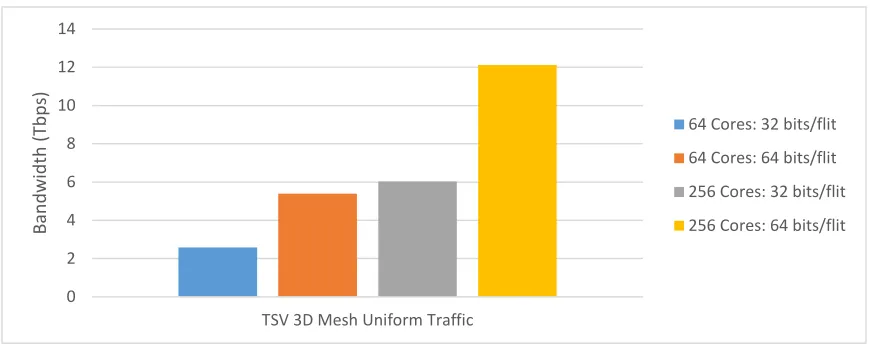
core has an equal probability to start sending a message to any other core. In Figure 3-3,
the peak bandwidths for 64 and 256 core systems that utilize 32 and 64 bits per flit are
[image:24.612.89.524.267.442.2]shown.
Figure 3-3: TSV Uniform Traffic Peak Bandwidth
When the system size is increased by a factor of 4, the peak bandwidth only
increases by a factor of approximately 2.3. This is likely due to an increase in the average
hop count when switching from the 4x4x4 to the 8x8x4 network configuration. The 64
core dense 3D mesh has an average hop count of 3.8095 while the 256 core dense 3D
mesh has an average hop count of 6.5255. The higher hop count results in more of the
packets reserving more of the overall network paths which reduces the peak bandwidth.
However, when the number of flits is doubled the peak bandwidth also doubles. This is
useful for increasing system performance but also results in higher chip area overheads 0
2 4 6 8 10 12 14
TSV 3D Mesh Uniform Traffic
B
a
n
d
w
id
th
(
T
b
p
s)
and energy dissipation. The effect that slowing down the vertical transmission times has
on uniform traffic bandwidth is explored in more detail in section 3.5.1.1.
3.3.2 Energy per Message
The average energy per packet measurement is started a thousand cycles after the
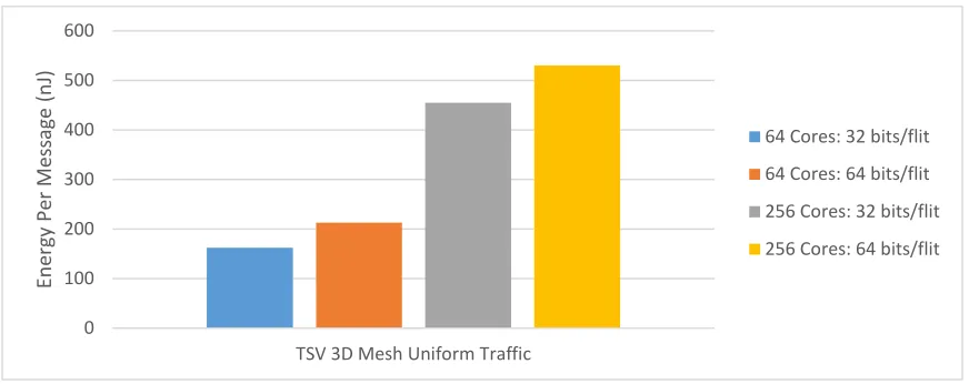
simulation begins to allow the network to settle. In Figure 3-4, the energy per message
[image:25.612.89.525.252.425.2]measurements for 64 and 256 core systems that use 32 and 64 bits per flit are shown.
Figure 3-4: TSV Uniform Traffic Energy per Message
When the packet size is doubled from 32 to 64 bits per flit, the average energy
dissipated per message only increases by 1.3 for the 64 core system and 1.2 for the 256
core system. This is a result of the increase of the energy dissipated by data transfer to
energy dissipated by waiting for network links to become free ratio when going from 32
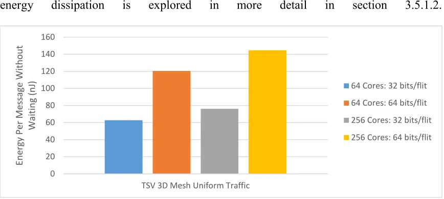
bits per flit to 64 bits per flit. The energy dissipated by the system for transferring data is
shown in Figure 3-5 where the energy from waiting is removed from the overall energy
measurements. When the system size increases from 64 to 256 cores, the energy
increases by 2.8 for sending packets with 32 bits per flit and 2.5 for sending packets with
64 bits per flit. Similar to the bandwidth differences, this is caused by the increase in 0
100 200 300 400 500 600
TSV 3D Mesh Uniform Traffic
E
n
e
rg
y
P
e
r
M
e
ss
a
g
e
(
n
J)
average hop count. The high network congestion also contributes to the increased
difference between the energy per message and the energy per message without waiting.
The effect that slowing down the vertical transmission times has on uniform traffic
[image:26.612.90.524.157.352.2]energy dissipation is explored in more detail in section 3.5.1.2.
Figure 3-5: TSV Uniform Traffic Energy per Message without Waiting
3.3.3 Network Latency
The average latency of a message is measured after one thousand cycles to allow
the network traffics to stabilize. It is calculated as the average difference between the
cycle numbers that the header flits were injected into the system and the cycle numbers
that the tail flits were absorbed by the destination cores. In Figure 3-6, the average
network latency measurements from header flit insertion to tail flit absorption are shown.
This shows an increase of a factor of 1.6 when scaling the number of cores from 64 to
256. Again, the average hop count contributes to the increased latency observed. The
high network congestion also significantly affects the overall latency. The effect that
decreasing the number of TSVs and slowing down the vertical transmission times has on 0 20 40 60 80 100 120 140 160
TSV 3D Mesh Uniform Traffic
E n e rg y P e r M e ss a g e W it h o u t W a it in g ( n
J) 64 Cores: 32 bits/flit
uniform traffic latency is explored in more detail in section 3.5.1.3.
Figure 3-6: TSV Uniform Traffic Average Latency
3.4. NoC Performance Evaluation with Non-Uniform Traffic
Non-uniform traffic patterns utilizing 64 cores were also explored to evaluate how
the network would perform with some common workloads and benchmarks. This gives a
better representation of the real world characteristics of the networks. The non-uniform
traffic patterns utilize extracted core to core communication frequencies for each
benchmark. BODYTRACK, CANNEAL, DEDUP, FFT, FLUIDANIMATE,
FREQMINE, LU, RADIX, SWAPTION, and VIPS benchmarks were used to
demonstrate the network performance of computationally intensive or communication
intensive workloads with the TSVs as the vertical connection technology.
3.4.1 Energy per Message
Similar to the measurements in Section 3.3.2, the average energy per packet
measurement is started a thousand cycles after the simulation begins to allow the network
to settle. In Figure 3-7, the energy per message measurements for 64 core systems that
use 32 and 64 bits per flit are shown. The average total energy dissipation from all of the 0
100 200 300 400 500 600 700 800
TSV 3D Mesh Uniform Traffic
La
te
n
cy
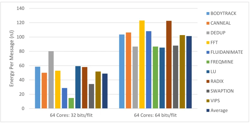
non-uniform traffic patterns doubles when shifting from 32 to 64 bits per flit as expected.
Figure 3-7: TSV Non-Uniform Traffic Energy per Message
Figure 3-8 shows the energy dissipation minus the energy used while waiting for
the network links to become free. It shows that there are very few instances where the
[image:28.612.89.526.398.631.2]network was congested for these non-uniform traffic patterns.
Figure 3-8: TSV Non-Uniform Traffic Energy per Message without Waiting
The energy dissipation is almost entirely from data transmission because the
network spends very little time waiting for the network to be free with these traffic 0 20 40 60 80 100 120 140
64 Cores: 32 bits/flit 64 Cores: 64 bits/flit
E n e rg y P e r M e ss a g e ( n J) BODYTRACK CANNEAL DEDUP FFT FLUIDANIMATE FREQMINE LU RADIX SWAPTION VIPS Average 0 20 40 60 80 100 120 140
64 Cores: 32 bits/flit 64 Cores: 64 bits/flit
patterns even with the more data intensive traffic patterns. Section 3.5.2.1 explores the
effect that slowing down the vertical transmissions for non-uniform traffic patterns has on
the overall energy dissipation.
3.4.2 Network Latency
The average latency of a message is measured after one thousand cycles to allow
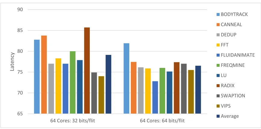
the network traffics to stabilize. In Figure 3-9, the average network latency measurements
from header flit insertion to tail flit absorption are shown. The variation in latency
between the 32 and 64 bits per flit simulations is caused by the inherent randomness in
the simulations. The single cycle transmission time for all network hops enables such low
latencies. The effect that slowing down the vertical transmission times for non-uniform
[image:29.612.89.522.388.602.2]traffic patterns has on the latency is explored in more detail in section 3.5.2.2.
Figure 3-9: TSV Non-Uniform Traffic Average Latency
3.5. TSV Density Analysis
Using the electrical characteristics of TSVs from [10], the energy required to
transfer a single bit through a TSV can be calculated for various pitches between the 65
70 75 80 85 90
64 Cores: 32 bits/flit 64 Cores: 64 bits/flit
La
te
n
cy
BODYTRACK CANNEAL DEDUP FFT
TSVs. As the pitch between the TSVs increases, the parasitic capacitance decreases and
therefore the energy required to transfer a bit is reduced. As long as the network is not
saturated and flits are not consistently waiting to be routed, the number of TSVs can be
reduced so that it takes multiple cycles to transmit a flit but the overall energy
consumption is lower and the area overhead of the TSVs is the same. By cutting the
number of TSVs per link in half, the pitch doubles, and it takes twice as long to transmit
the flit through that link.
3.5.1 NoC Performance Evaluation
The TSV density analysis is done by simulating the 64 and 256 core networks
with enough TSVs per vertical link to transfer an entire flit in one, two, and four cycles.
When working with 32 bit flits, that requires 32, 16, and 8 TSVs respectively. Likewise,
with 64 bit flits, 64, 32, and 16 TSVs were used. Using the same Π model from [10], the
full number of TSVs each use 17.459 fJ/bit again, half the number of TSVs take 9.2078
fJ/bit, while half again the number of TSVs only utilize 6.1044 fJ/bit. This shows a
diminishing return in cutting the number of TSVs.
3.5.1.1
Bandwidth
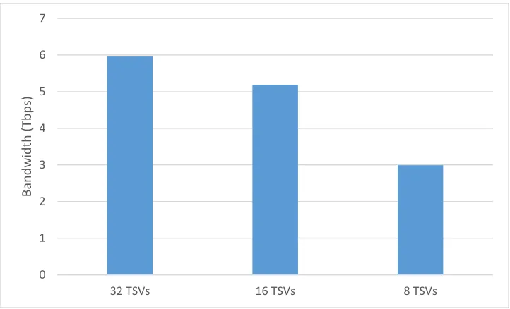
The peak bandwidth for 64 and 256 core systems with increasing flit vertical
transmit times is shown in Figure 3-10 and Figure 3-11. If the TSVs are designed so that
they take two cycles to transmit a flit between layers, then the 64 core systems do not end
up with much of a peak performance hit, which is desirable. The 256 core systems show
an increase in peak bandwidth when the vertical transmit times are doubled, indicating
performance of the system and that the vertical transmission speed can be decreased to
achieve higher bandwidth and increased energy efficiency. If the number of chip layers is
increased, the TSVs become the bottleneck for the network performance. To show this,
two simulations are run with a NoC in an 8x4x8 configuration and an 8x8x8
configuration in Figure 3-12 and Figure 3-13 respectively. The increased number of chip
layers results in the expected decrease in performance.
Figure 3-10: TSV Density Analysis with 32 bits/flit Uniform Traffic Peak Bandwidth
Figure 3-11: TSV Density Analysis with 64 bits/flit Uniform Traffic Peak Bandwidth 0 1 2 3 4 5 6 7 8
32 TSVs 16 TSVs 8 TSVs
B a n d w id th ( T b p s)
64 Core Uniform 32 bits/flit 256 Core Uniform 32 bits/flit
0 2 4 6 8 10 12 14 16
64 TSVs 32 TSVs 16 TSVs
B a n d w id th ( T b p s)
Figure 3-12: TSV Density Analysis with an 8x4x8 NoC and 32 bits/flit Uniform Traffic
Figure 3-13: TSV Density Analysis with an 8x8x8 NoC and 32 bits/flit Uniform Traffic
3.5.1.2
Energy per Message
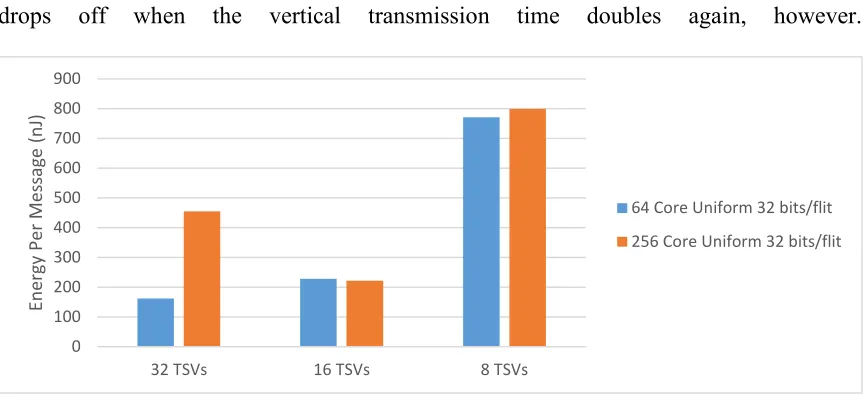
The energy per message measurements for varying the number of TSVs are
shown in Figure 3-14 and Figure 3-15. In both the 32 bits per flit and the 64 bits per flit
simulations, transitioning from one cycle to two cycles to transmit a flit between layers, 0
1 2 3 4 5 6 7
32 TSVs 16 TSVs 8 TSVs
B
a
n
d
w
id
th
(
T
b
p
s)
0 2 4 6 8 10 12
32 TSVs 16 TSVs 8 TSVs
B
a
n
d
w
id
th
(
T
b
p
s)
[image:32.612.123.489.314.542.2]the 64 core systems consume slightly more energy when the network is fully loaded. This
is because of the excess waiting that occurs whereas the 256 core systems have better
energy efficiency when the vertical transmissions take an extra cycle. The effect quickly
drops off when the vertical transmission time doubles again, however.
[image:33.612.91.525.154.357.2]Figure 3-14: TSV Density Analysis with 32 bits/flit Uniform Traffic Energy per Message
Figure 3-15: TSV Density Analysis with 64 bits/flit Uniform Traffic Energy per Message
Figure 3-16 and Figure 3-17 show the average energy dissipated per message
without the waiting energy. Both the 32 bits/flit and 64 bits/flit simulations show that the
data transmission energy levels off when the vertical data transfers take two cycles. The
four cycle transmission time also shows a large disparity between the total energy per 0 100 200 300 400 500 600 700 800 900
32 TSVs 16 TSVs 8 TSVs
E n e rg y P e r M e ss a g e ( n J)
64 Core Uniform 32 bits/flit 256 Core Uniform 32 bits/flit
0 100 200 300 400 500 600 700 800 900 1000
64 TSVs 32 TSVs 16 TSVs
E n e rg y P e r M e ss a g e ( n J)
message and the energy per message without the waiting component.
Figure 3-16: TSV Density Analysis with 32 bits/flit Uniform Traffic Energy per Message without Waiting
Figure 3-17: TSV Density Analysis with 64 bits/flit Uniform Traffic Energy per Message without Waiting
3.5.1.3
Latency
The average packet latency measurements are shown in Figure 3-18 and Figure
3-19. For 64 core systems one extra cycle for vertical transmissions in a saturated
network causes the latency to increase. With 256 core systems however, the latency
increase is not as noticeable. This effect also drops off when the transmission time of a
flit doubles again and the latency increases significantly. 0 10 20 30 40 50 60 70 80
32 TSVs 16 TSVs 8 TSVs
E n e rg y P e r M e ss a g e W it h o u t W a it in g ( n J)
64 Core Uniform 32 bits/flit 256 Core Uniform 32 bits/flit
0 20 40 60 80 100 120 140 160
64 TSVs 32 TSVs 16 TSVs
E n e rg y P e r M e ss a g e W it h o u t W a it in g ( n J)
Figure 3-18: TSV Density Analysis with 32 bits/flit Uniform Traffic Average Latency
Figure 3-19: TSV Density Analysis with 64 bits/flit Uniform Traffic Average Latency
3.5.2 NoC Performance Evaluation with Non-Uniform Traffic
Similar to the uniform traffic simulations, the same non-uniform traffic
simulations from section 3.4 are also performed with vertical data transfers taking one,
two, and four cycles.
3.5.2.1
Energy per Message
The energy per message for non-uniform traffic is shown in Figure 3-20 for the 32
bits/flit simulations and Figure 3-21 for the 64 bits/flit simulations. Cutting the number of 0
200 400 600 800 1000 1200 1400
32 TSVs 16 TSVs 8 TSVs
La
te
n
cy
64 Core Uniform 32 bits/flit 256 Core Uniform 32 bits/flit
0 200 400 600 800 1000 1200 1400
64 TSVs 32 TSVs 16 TSVs
La
te
n
cy
TSVs in half results in a reduction in the energy dissipation for most of the traffic
patterns. A further reduction in the TSV count does not appear to reduce the energy
dissipation much if at all. This is a result of the increased energy spent waiting on the
network links to become free. There is a minimum point where a reduced number of
TSVs allows for the minimum energy. Too few or too many TSVs and the energy
increases again because the amount of energy waiting for the slower vertical links
outweighs the energy savings from spreading the TSVs out.
Figure 3-20: TSV Density Analysis with 32 bits/flit Non-Uniform Traffic Energy per Message
Figure 3-21: TSV Density Analysis with 64 bits/flit Non-Uniform Traffic Energy per Message 0 10 20 30 40 50 60 70 80 90
32 TSVs 16 TSVs 8 TSVs
E n e rg y P e r M e ss a g e ( n J) BODYTRACK CANNEAL DEDUP FFT FLUIDANIMATE FREQMINE LU RADIX SWAPTION VIPS 0 20 40 60 80 100 120 140
64 TSVs 32 TSVs 16 TSVs
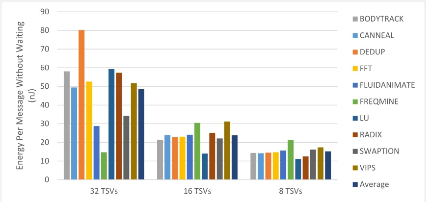
Figure 3-22 and Figure 3-23 show the average energy per message minus the
energy spent waiting for the network. These graphs show a general trend of the
diminishing returns that increasing the pitch between the TSVs cause. There is also a
larger difference between the total energy per message and the energy per message
[image:37.612.89.527.209.415.2]without waiting. This is a direct result of the increased vertical transmission times.
[image:37.612.89.525.447.658.2]Figure 3-22: TSV Density Analysis with 32 bits/flit Non-Uniform Traffic Energy per Message without Waiting
Figure 3-23: TSV Density Analysis with 64 bits/flit Non-Uniform Traffic Energy per Message without Waiting 0 10 20 30 40 50 60 70 80 90
32 TSVs 16 TSVs 8 TSVs
E n e rg y P e r M e ss a g e W it h o u t W a it in g (n J) BODYTRACK CANNEAL DEDUP FFT FLUIDANIMATE FREQMINE LU RADIX SWAPTION VIPS Average 0 20 40 60 80 100 120 140
64 TSVs 32 TSVs 16 TSVs
3.5.2.2
Latency
The latency for non-uniform traffic is shown in Figure 3-24 and Figure 3-25.
These show that the latency increases slightly when switching from one cycle to two
cycles of vertical data transmission, but that it increases significantly more when going to
four cycles. The increased vertical transmission times have a direct impact on the latency
[image:38.612.90.529.243.455.2]measurements.
Figure 3-24: TSV Density Analysis with 32 bits/flit Non-Uniform Traffic Average Latency
Figure 3-25: TSV Density Analysis with 64 bits/flit Non-Uniform Traffic Average Latency 0 50 100 150 200 250 300
32 TSVs 16 TSVs 8 TSVs
La te n cy BODYTRACK CANNEAL DEDUP FFT FLUIDANIMATE FREQMINE LU RADIX SWAPTION VIPS Average 0 50 100 150 200 250 300
64 TSVs 32 TSVs 16 TSVs
[image:38.612.90.524.484.695.2]3.6. Area Overheads
To prevent capacitive coupling the TSVs are shielded with neighboring TSVs.
This results in an overall chip area overhead for the 32 bit flit of at least 12500µm2 using
a 5µm radius and a base pitch of 20µm depending on the configuration. For 64 bit flits, at
least 25500µm2 are required for the TSVs. A 64 core network will need to dedicate a total
of 0.8mm2 for 32 bits per flit and 1.632mm2 for 64 bits per flit. A 256 core network will
require 3.2mm2 for 32 bits per flit and 6.528mm2 for 64 bits per flit. These TSVs require
Chapter 4
Wireless 3D NoC Architectures
Four network architecture and wireless vertical connection technology pairs are
compared: capacitive coupling with a dense 3D mesh network, inductive coupling with a
dense 3D mesh network, inductive coupling with a ring network based on [18], and
inductive coupling with a proposed sparse mesh network described later in this section.
The dense 3D mesh network was introduced in section 3.1 for the wired TSV networks.
Capacitive coupling requires that two chip layers be assembled in a face to face
configuration. Therefore, the capacitive coupling mesh network for 64 cores is in an
8x4x2 configuration and for 256 cores is in a 16x8x2 configuration for these simulations.
Other than the restriction that the number of planes is limited to two, the dense 3D mesh
network is similar to the NoC described in section 3.1. Using designs mentioned in [12],
the capacitive coupling links consume 15 fJ/bit and take 23 and 46 clock cycles to
transfer a 32 and 64 bit flit respectively.
Inductive coupling does not have the face to face restriction and can have more
than two chip layers. For the inductive coupling links, using designs from [11], energy
consumption is 140 fJ/bit and it takes 3 cycles for 32 bit flits and 6 cycles for 64 bit flits.
The dense 3D mesh inductive coupling networks were in 4x4x4 and 8x8x4 configurations
for the 64 and 256 core systems respectively. This network architecture is also similar to
the NoC described in section 3.1. The ring network originally described in [18] has
vertical connections on either side of the chip as shown in Figure 4-1. The 256 core
version is similar. The sparse 3D mesh network is for the 4x4x4 64 core network and has
three inductive coupling links for each group of four cores on each layer to facilitate
times for 32 bit flits and two cycle transmissions times for 64 bit flits. It also reduces the
number of inductive coupling links required for each group of four cores by one, which
saves valuable chip area. There are extra connections between cores such that any core
takes at most one hop to reach a switch that has a vertical connection. The cores central to
the chip contain the vertical connections. This allows for the large area of the inductive
coupling circuit to be implemented so that inductive coupling pairs have minimal
[image:41.612.252.360.297.436.2]coupling impact on each other. One layer of the sparse 3D mesh network is shown in
Figure 4-2.
[image:41.612.246.366.507.665.2]Figure 4-1: 3D Ring NoC
4.1. Performance Evaluation
The same performance metrics described in section 3.2 are utilized for the
wireless 3D NoC architecture simulations. Bandwidth, energy per message, and latency
measurements with uniform and non-uniform traffic for each technology and architecture
pair are compared.
4.1.1 Bandwidth
The peak system bandwidth for the wireless vertical connection technologies are
shown in Figure 4-3 and Figure 4-4. The inductive coupling mesh networks have a higher
system bandwidth than the capacitive coupling mesh network. This is mostly a result of
the very high vertical communication times for the capacitive coupling architecture even
though the majority of the data transfers are within the same layer. The average hop
counts for the capacitive coupling networks are also higher than the other wireless
networks as can be seen in Table 4-1. The inductive coupling sparse mesh lags behind the
dense mesh but outperforms the ring and the capacitive coupling mesh networks. Next to
the TSV vertical connections however, the wireless connections have a lower peak
bandwidth. Comparing the quickest wired architectures discussed in section 3.5.1.1 and
wireless architectures for the 64 core networks with 32 bits per flit the inductive coupling
dense 3D mesh has a peak bandwidth 35% lower than the 32 TSV dense 3D mesh. With
the 256 core networks and 32 bits per flit, the inductive coupling dense 3D mesh network
is 10% slower than the 16 TSV dense 3D mesh. When analyzing the wireless 32 and 64
bits per flit simulations, the serial communication of both the inductive and capacitive
coupling technologies does not scale well with increasing flit size compared to the wired
the bandwidth per link for 64 bits/flit is compared in Table 4-3. These bandwidth per link
calculations help depict why the peak bandwidth varies between the technologies and
architectures.
Figure 4-3: Wireless Comparison with 32 bits/flit Uniform Traffic Peak Bandwidth
Figure 4-4: Wireless Comparison with 64 bits/flit Uniform Traffic Peak Bandwidth
Technology/Architecture Pair Average Hop Count 64 Core Capacitive Coupling Dense 3D Mesh 4.4444 256 Core Capacitive Coupling Dense 3D Mesh 8.4706 64 Core Inductive Coupling Dense 3D Mesh 3.8095
256 Core Inductive Coupling Dense 3D Mesh 6.5255 64 Core Inductive Coupling Ring 4.1905 256 Core Inductive Coupling Ring 7.8431 64 Core Inductive Coupling Sparse 3D Mesh 3.9524
Table 4-1: Technology and Architecture Pairs System Average Hop Count Comparison 0 1 2 3 4 5 6 7 Capacitive Coupling Dense Mesh Inductive Coupling Dense Mesh Inductive Coupling Ring Inductive Coupling Sparse Mesh B a n d w id th ( T b p s)
64 Cores: 32 bits/flit 256 Cores: 32 bits/flit
0 1 2 3 4 5 6 7 8 9 Capacitive Coupling Dense Mesh Inductive Coupling Dense Mesh Inductive Coupling Ring Inductive Coupling Sparse Mesh B a n d w id th ( T b p s)
Technology/Architecture Pair
Bandwidth per Link with 32
bits/flit (Gbps) Vertical Cycles for 32 bits/flit
32 TSV Dense 3D Mesh 80 1
16 TSV Dense 3D Mesh 40 2
8 TSV Dense 3D Mesh 20 4
Capacitive Coupling Dense 3D Mesh 3.47826087 23
Inductive Coupling Dense 3D Mesh 26.66666667 3
Inductive Coupling Ring 26.66666667 3
Inductive Coupling Sparse 3D Mesh 80 1
Table 4-2: Technology and Architecture Pairs 32 bits/flit System Bandwidth Comparison
Technology/Architecture Pair
Bandwidth per Link with 64
bits/flit (Gbps) Vertical Cycles for 64 bits/flit
64 TSV Dense 3D Mesh 160 1
32 TSV Dense 3D Mesh 80 2
16 TSV Dense 3D Mesh 40 4
Capacitive Coupling Dense 3D Mesh 3.47826087 46
Inductive Coupling Dense 3D Mesh 26.66666667 6
Inductive Coupling Ring 26.66666667 6
[image:44.612.88.526.72.206.2]Inductive Coupling Sparse 3D Mesh 80 2
Table 4-3: Technology and Architecture Pairs 64 bits/flit System Bandwidth Comparison
4.1.2 Energy per Message
The energy per message for the wireless connection architectures are compared in
Figure 4-5 and Figure 4-6. The capacitive coupling network consumes a considerable
amount of energy compared to the other network architecture and technology pairs except
for the inductive coupling ring with 256 cores. As Table 4-2 and Table 4-3 show, each
capacitive coupling link takes several more clock cycles than any of the other architecture
technology pairs causing the network to become congested. The inductive coupling ring
with 256 cores spends a considerable amount of time waiting on network congestion as a
result of the ring architecture. Highly congested networks spend more time and energy
mesh network consumes less energy than the ring network but is less efficient than the
inductive coupling dense mesh network. For the sparse mesh network, three times as
much energy is dissipated in a single cycle for the vertical transmissions compared to the
other inductive coupling networks. It makes up for the increased energy consumption in
one cycle by decreasing the overall latency. In a fully loaded network, the four switches
in a layer that handle the vertical transmissions are traffic hotspots that bottleneck the
system and dissipate extra energy compared to the dense mesh network. For each of the
networks other than the ring architecture, the energy per message for 256 core networks
does not change much from the 64 core networks because the number of vertical
transmissions per message are similar. The 256 core ring network, however, spends a lot
of time waiting for the vertical links to be free. When comparing flit sizes of 32 and 64
bits for each architecture, the energy per message approximately doubles due to the
limitations of the wireless serial communications and their poor scaling.
Figure 4-5: Wireless Comparison with 32 bits/flit Uniform Traffic Energy per Message 0 500 1000 1500 2000 2500 3000 3500 4000 4500 Capacitive Coupling Dense Mesh Inductive Coupling Dense Mesh Inductive Coupling Ring Inductive Coupling Sparse Mesh E n e rg y P e r M e ss a g e ( n J)
Figure 4-6: Wireless Comparison with 64 bits/flit Uniform Traffic Energy per Message
Figure 4-7 and Figure 4-8 show the energy consumption of just the data
transmission. Most of the wireless architecture and technology pairs dissipate the
majority of their energy per message waiting for the network. The capacitive coupling
mesh network has a higher energy dissipation because of the slow link speeds. The 64
core inductive coupling ring network spends about 20% of the energy on data because of
the high network congestion. The 256 core ring network is even worse with 9%. The
inductive coupling dense mesh dissipates about 30% of the energy per message in the
data transmissions. The sparse mesh inductive coupling network on the other hand spends
more energy on transferring data than the other architecture and technology
combinations. It dissipates about 50% of the total energy per message in the data
transmissions and is the most efficient from a wasted energy point of view. The
efficiencies for networks using 64 bits per flit are worse than networks using 32 bits per
flit again because of the increased network congestion and poor scaling. 0 1000 2000 3000 4000 5000 6000 7000 8000 9000 10000 Capacitive Coupling Dense Mesh Inductive Coupling Dense Mesh Inductive Coupling Ring Inductive Coupling Sparse Mesh E n e rg y P e r M e ss a g e ( n J)
Figure 4-7: Wireless Comparison with 32 bits/flit Uniform Traffic Energy per Message without Waiting
Figure 4-8: Wireless Comparison with 64 bits/flit Uniform Traffic Energy per Message without Waiting
4.1.3 Latency
The latency from header flit insertion to tail flit absorption is shown in Figure 4-9
and Figure 4-10. The sparse mesh network has a lower latency than the other inductive
coupling networks. The single cycle vertical transmission time compared to the longer
transmission times of the other architectures as described in Table 4-2, enables the sparse
mesh architecture to maintain lower latencies. It has slightly less of an advantage
compared to the capacitive coupling mesh network because the majority of the capacitive
coupling communications occur within the same chip layer even though the capacitive 0 50 100 150 200 250 300 350 400 450 500 Capacitive Coupling Dense Mesh Inductive Coupling Dense Mesh Inductive Coupling Ring Inductive Coupling Sparse Mesh E n e rg y P e r M e ss a g e W it h o u t W a it in g ( n J)
64 Cores: 32 bits/flit 256 Cores: 32 bits/flit
0 100 200 300 400 500 600 700 Capacitive Coupling Dense Mesh Inductive Coupling Dense Mesh Inductive Coupling Ring Inductive Coupling Sparse Mesh E n e rg y P e r M e ss a g e W it h o u t W a it in g ( n J)
[image:47.612.90.522.294.461.2]links take several more cycles to transmit each individual flit between chip layers. The
inductive coupling sparse 3D mesh actually has a higher latency than the capacitive
coupling dense mesh when using 64 bits per flit. In practice the network is usually not as
saturated as it is with uniform traffic. Non-uniform traffic patterns give a better
representation of a real application’s communication latency and is explored in more
[image:48.612.87.525.209.400.2]detail for the wireless architectures in section 4.2.2.
Figure 4-9: Wireless Comparison with 32 bits/flit Uniform Traffic Average Latency
Figure 4-10: Wireless Comparison with 64 bits/flit Uniform Traffic Average Latency
4.2. Performance Evaluation with Non-Uniform Traffic
Similar to section 3.4, the NoCs are also compared with common non-uniform
traffic patterns. Analysis of the energy per message and latency is done for all of the 0 200 400 600 800 1000 1200 1400 Capacitive Coupling Dense Mesh Inductive Coupling Dense Mesh Inductive Coupling Ring Inductive Coupling Sparse Mesh La te n cy
64 Cores: 32 bits/flit 256 Cores: 32 bits/flit
0 200 400 600 800 1000 1200 1400 Capacitive Coupling Dense Mesh Inductive Coupling Dense Mesh Inductive Coupling Ring Inductive Coupling Sparse Mesh La te n cy
[image:48.612.88.524.432.599.2]wireless architectures with the benchmarks BODYTRACK, CANNEAL, DEDUP, FFT,
FLUIDANIMATE, FREQMINE, LU, RADIX, SWAPTION, and VIPS.
4.2.1 Energy per Message
The energy per message for non-uniform traffic is compared in Figure 4-11 and
Figure 4-12. Similar to the uniform traffic results in section 4.1.2, the sparse mesh
network in practice consumes considerably more energy than the other networks. The
capacitive coupling simulations vary widely depending on which traffic patterns tried to
send data over the vertical connections, but overall consumed more energy than the
inductive coupling dense mesh and ring networks. For traffic patterns utilizing 64 bits
per flit, the capacitive coupling network consumes more energy per message than even
the sparse 3D mesh. As depicted in Table 4-2 and Table 4-3, the high vertical
transmission time contributes to a congested network for traffics that send data from one
end of the chip to the other. The inductive coupling ring and mesh networks had similar
energy dissipation. The energy saving benefits of having fewer inductive coupling links
[image:49.612.90.524.530.690.2]in the ring network is balanced by the reduced waiting time of the dense 3D mesh.
Figure 4-12: Wireless Comparison with 64 bits/flit Non-Uniform Traffic Energy per Message
Figure 4-13 and Figure 4-14 show the energy dissipation without waiting. The
capacitive coupling network energy dissipation is mostly from waiting on the vertical
connections because of the extended vertical transmission times and high network
congestion. The inductive coupling networks rarely required any waiting so the energy
dissipation without waiting is close to the overall energy dissipation. The ring network
has the greatest energy dissipation disparity, with the dense 3D mesh closely following.
The sparse 3D mesh has the least disparity between the two measurements and spends
[image:50.612.90.523.463.675.2]most of the overall energy transferring data between each of the cores.
Figure 4-14: Wireless Comparison with 64 bits/flit Non-Uniform Traffic Energy per Message without Waiting
4.2.2 Latency
The average latency for the non-uniform traffic patterns are shown in Figure 4-15
and Figure 4-16. The inductive coupling sparse mesh does really well performance wise
and is only slightly behind the quickest TSV results while outperforming the slower TSV
networks that use 32 bits per flit and staying competitive with the slower TSV networks
that use 64 bits per flit. The energy increase for typical workloads may not be worth the
performance increase compared to the other inductive coupling networks. For instances
where a wireless interconnect is essential, such as the implementation of a liquid cooling
layer, the sparse 3D mesh could be the best option to maintain similar vertical
performance to the rest of the chip using TSVs. The capacitive coupling mesh does not
perform as well. It consumes a lot of extra energy and the latency is significantly higher
compared to all of the inductive coupling networks. The high vertical transmission time
as illustrated by Table 4-2 and Table 4-3 is the main contributor to the excess latency
slightly slower than the full 3D mesh. The network congestion at the inductive coupling
[image:52.612.88.525.126.339.2]links and the higher average hop count plays a role in the increased latency.
Figure 4-15: Wireless Comparison with 32 bits/flit Non-Uniform Traffic Average Latency
Figure 4-16: Wireless Comparison with 64 bits/flit Non-Uniform Traffic Average Latency
4.3. Area Overheads
According to [11] and [12], each capacitive coupling transceiver would require at
least 320µm2 and each inductive coupling transceiver would need at least 900 µm2. As
[image:52.612.89.523.368.580.2]smaller than the required area for TSVs. These wireless technologies also do not require
any additional manufacturing steps, unlike TSVs.
Technology/Architecture Pair Per Link Chip Area (um2) 64 Core Total Chip Area (um2) 256 Core Total Chip Area (um2)
TSV Dense 3D Mesh 32
bits/flit 12500 800000 3200000
TSV Dense 3D Mesh 64
bits/flit 25500 1632000 6528000
Capacitive Coupling Dense
3D Mesh 320 20480 81920
Inductive Coupling Dense 3D
Mesh 900 57600 230400
Inductive Coupling Ring 900 28800 57600 Inductive Coupling Sparse 3D
Mesh 900 14400 N/A
Chapter 5
Conclusions
5.1. Summary
The TSV 3D mesh has the highest bandwidth, lowest energy consumption, and
lowest latency of all of the network architectures. Of the wireless architectures, the
inductive coupling dense 3D mesh had the highest bandwidth and lowest energy, but the
inductive coupling sparse 3D mesh maintained a much lower latency. If wireless
interconnects are not required and manufacturing permits, a TSV 3D mesh would be
ideal. When choosing between wireless architectures, inductive coupling is better than
capacitive coupling but which architecture to use will depend on the design constraints.
An energy constrained system would benefit more from a dense 3D mesh while a latency
constrained system would benefit more from a sparse 3D mesh.
5.1.1 System Bandwidth
In a system bandwidth comparison, the wired TSV mesh outperforms all of the
wireless architectures by at least 54.874% for 64 cores and 32 bits per flit. It also
outpaces the wireless architectures by at least 187.296% for 64 cores and 64 bits per flit
because of the relatively low bits per flit scalability of the wireless architectures. For 256
cores and 32 bits per flit, the wired TSV mesh is 11.613% faster than the wireless
architectures only if the number of TSVs is cut in half so that vertical transmissions of
flits take two clock cycles. Similarly, for 256 cores and 64 bits per flit, the 32 TSV wired
mesh is 82.662% faster than the wireless architectures. The number of chip layers also
vertical transmission time and high vertical connectivity contribute to the TSVs high
bandwidth performance.
When analyzing just the wireless architectures, the inductive coupling dense 3D
mesh is 46.598% faster than the inductive coupling sparse 3D mesh, 85.565% faster than
the inductive coupling ring, and 220.428% faster than the capacitive coupling mesh
network with 64 cores and 32 bits per flit. With 256 cores and 32 bits per flit, the
inductive coupling dense 3D mesh is 191.502% faster than the capacitive coupling
network and 253.52% faster than the inductive coupling ring network. Similarly with 64
cores and 64 bits per flit, the inductive coupling dense 3D mesh is 55.499% faster than
the inductive coupling sparse 3D mesh, 82.012% faster than the inductive coupling ring,
and 167.346% faster than the capacitive coupling 3D mesh. With 256 cores and 64 bits
per flit, the inductive coupling dense 3D mesh is 173.901% faster than the capacitive
coupling network and 278.162% faster than the inductive coupling ring. With 64 and 256
cores, the lower vertical transmission times and high vertical connectivity help the
inductive coupling dense 3D mesh maintain the highest bandwidth. With 256 cores, the
longer vertical transmission times for the capacitive coupling network is balanced with
the increased percentage of same layer packet transmissions that lead to higher
bandwidths than the inductive coupling ring.
5.1.2 System Energy per Message
Analyzing the energy per message for uniform traffic patterns with 32 bits per flit
and 64 cores, the TSV mesh has a 75.359% reduction in energy consumption compared
to the inductive coupling dense 3D mesh. With 64 bits per flit and 64 cores, the TSV
coupling sparse 3D mesh. Similarly, the 32 TSV 256 core system with 32 bits per flit
shows a 62.1% reduction in energy from the inductive coupling dense 3D mesh. The 32
TSV 256 core system with 64 bits per flit has an 88.321% decrease in energy compared
to the inductive coupling dense 3D mesh. As a technology, the TSVs are better at scaling
both the number of bits per flit and the number of cores in the system than the wireless
architectures.
In a pure wireless architecture comparison with 64 cores and 32 bits per flit, the
inductive coupling dense 3D mesh uses 30.183% less energy than the inductive coupling
sparse 3D mesh, 35.541% less energy than the inductive coupling ring, and 83.367% less
than the capacitive coupling network. With 64 bits per flit, the inductive coupling sparse
3D mesh uses 5.296% less energy than the inductive coupling dense mesh, has a
34.921% reduction compared to the inductive coupling ring, and 68.049% less than the
capacitive coupling mesh. Looking at 256 core wireless systems with 32 bits per flit, the
inductive coupling dense 3D mesh has an 84.303% decrease in energy per message
compared to the capacitive coupling mesh and an 85.324% reduction compared to the
inductive coupling ring network. For 256 cores and 64 bits per flit, the inductive coupling
dense 3D mesh uses 69.11% less energy than the capacitive coupling 3D mesh and
78.391% less energy than the inductive coupling ring. In general, the inductive coupling
dense 3D mesh uses less energy than the other networks except for 64 cores and 64 bits
per flit at which point the inductive coupling sparse mesh has a slight edge. The two
cycle transmission times help the network use less energy than the six cycle transmission
tim