Remediation of petroleum-contaminated Antarctic soil
BY
SUSAN HARRIET FERGUSON J.P.
B.App. Sci. — University of Canberra
B Ant. Stud. (Hons) — University of Tasmania
Submitted in fulfilment of the requirements for the Degree of
Doctor of Philosophy
University of Tasmania
A thesis submitted in fulfilment of the requirements of Doctor of Philosophy School of Geography and Environmental Studies
Declaration
Except as stated herein, this thesis contains no material which has been accepted for the award of any other degree or diploma in a tertiary institution, and to the best of my
knowledge and belief, contains no material previously published or written by another person, except when due reference is made.
for
All my wonderful family
The love and support you have given me has allowed me to create wonderful dreams ....and then make them real
Thank you
And
The Wombles - if we would only follow their lead
Underground, overground, wombring free, The Wombres of Wimbledon Common are we. Maf4ng good use of the things that we find, 'Things that the everyday folks leave behind
Uncle Bu&aria,
9-& can remember the days when Tie wasn't be/lindthe times, With his map of the world.
Pickup the papers and take them to Tobermory! Wombles are organised, workjis a team. Wombles are tidy and Wombres are clean. Underground, overground, wombling free, 'The Wombres of Ttimbredon Common are we!
People don't notice us, they never see, Under their noses a Womble may be. We womble by nht and we womble by day,
Loong for fitter to trundle away. We're so incredibly, utterly devious gtfang the most of everything.
Even bottles and tins.
Pickup the pieces and make them into something new, Is what we do!
Underground, overground wombling free, The Wombres of Wimbledon Common are we.
Acknowledgements
Acknowledgement for this study must go to my (cast of thousand) supervisors, Dr. Ian Snape, Dr. Peter Franzmann, Dr. Andrew Revill and Dr. Richard Coleman. As 'The Franzmann' liked to quote "without grit you can have no pearl".., you were all very (extremely) gritty.
During the time that it has taken me to complete this thesis, I've been fortunate to have many wondrous and amazing experience. Among the (too many to name) highlights - the best joy (ah-hem I mean maintenance) helicopter flight on my birthday in Antarctica — oh and all that diamond dust, waiting for a family of Emus on the Nullarbor, drinking warm ale with Jenny and Clare at a poky tavern in Cambridge (The Rat and Parrot), feeding the Archer fish on the Ord River and swimming in the (warm) Southern Ocean at Esperance. For these experiences I want to thank my family, friends and colleagues.
To all of the people who made the work more manageable: Dr. Michael Trefry, Dr. Ben Raymond, Rebecca Esmay, John Rayner, Dr. Steve Fisher, Dr. John Gibson, Andrei Woinarski, Shane Powell and Paul Harvey. The friends that where there even when they didn't quite understand why: Steven Whichelo, Richard Coleman, Shavawn Donoghue, Sandra Hodgson, Peter Deith and Mark Anderson to name just a few
The numerous and various housemates who had to put up with all the highs and lows: Gareth Stephenson, Scott Ayres, Dave Connell, Ben Fowler, Bronwen Butcher, Sean Westbrook, Alison McMorrow, Matt Paget, The Pink Room People and all the people who I "shared" with in Antarctica.
Special thanks to Brett Quinton, who may have joined the team in the final innings but made the last months very enjoyable.
For the cuddles when it was all too much or just because: Meg, Molly, Rama, and Tilda
Many thanks to the Antarctic Division (Kingston), CSIRO (Hobart and Perth) and ANARE for the use of their research facilities and field support in Antarctica. This research could not be completed without support from ASAC Grant No 1163
The following people and institutions contributed to the publication of the work undertaken as part of this thesis:
Ferguson, S. H., Franzmann, P. D., Snape,
I.,Revill, A. T., Trefry, M. G., Zappia, L.
R., 2003. Effects of temperature on mineralisation of petroleum in contaminated
Antarctic terrestrial sediments. Chemosphere. 52(6), 975-987.
Ferguson, S. H., Franzmann,
P. D.,Revill, A. T., Snape, I., Rayner, J. L., 2003. The
effects of nitrogen and water on mineralisation of diesel-contaminated terrestrial
Antarctic soils. Cold Regions Science and Technology. 37(2), 197-212.
Ferguson, S. H., Woinarski, A. Z., Snape, I., Morris, C. E., Revill, A. T., In Press. A
field trial of In Situ Chemical Oxidation (ICO) to remediate long-term diesel
contaminated Antarctic soil. Cold Regions Science and Technology.
• Ferguson, S. H., Powell, S. M., Snape,
I.,Gibson, J. A. E. Franzmann P.D.,
Submitted. Effect of temperature on the microbial ecology of a
hydrocarbon-contaminated Antarctic soil: Implications for high temperature remediation. FEMS
Microbial Ecology.
Ferguson S.
H.,Franzmann P. D., Snape I, Zappia L. R. 2000. Determination of
temperature effects on mineralisation of diesel-contaminated Antarctic sediments using
14
C-octadecane. 2nd International Conference on Contaminants in Freezing Ground, July
2-5, 2000, Cambridge, UK.
Ferguson S.
H.,Revill A. T., Snape I, Franzmann P. D. 2002. Comparison of
microbial mineralisation of petroleum hydrocarbons in Antarctic sediments by
radiometric experiments and gas chromatography. Proceedings of the Australian
Organic Geochemistry Conference. 12-15 February 2002, Hobart, Australia.
Ferguson S.
H.,Franzmann P. D., Snape I, Revill A. T., Zappia LR. 2002. The effect
of nutrients and water availability on mineralisation of diesel-contaminated Antarctic
sediments as determined by "C-octadecane microcosm experiments. Proceedings of the
3rd International Conference on Contaminants in Freezing Ground, 14-18 April 2002,
Hobart, Australia.
Snape, I., Ferguson, S. H., Harvey,
P.,Revill, A. T., Submitted. Chemical constraints
on natural attenuation of fuel spills at Casey Station, Antarctica. Chemosphere.
Snape, I., Ferguson, S.
H.,Revill, A. T., 2003. Constraints on rates of natural
attenuation and
in situbioremediation of petroleum spills in Antarctica. In: Nahir, M.,
Bigger, K. Cotta, G (Eds.)
Assessment and remediation of contaminated sites in Arctic and cold climates (ARCSACC)Edmonton, Canada, May 4-6.
I Snape
P. D. Franzmann
A. T. Revill
C. E. Morris
L. R. Zappia
M. G. Trefry
J. L. Rayner
S. M. Powell
J. A. E. Gibson
A. Z. Woinarski
P. Harvey
/c.-- -I-7—
7ttfr
li
/
-
i
NaArn
Snape I, Ferguson S. H., Franzmann P. D., Morris C. E., Revill A. T. 2000. Contaminants in the Antarctic Environment VII: Remediation of petroleum hydrocarbons. In: Hughson T., Ruckstuhl C. (Eds.). Proceedings of the 6th International Symposium on Cold Region Development (ISCORD): 148-150.
• I. Snape, P. Franzmann and A. Revill assisted with guidance and general supervision in all aspects of producing publishable quality manuscripts
• Molecular biology (DGGE and 16S rRNA gene sequencing) by S. Powell • J. Gibson assisted in phospholipid interpretation and re-analysis of isolate
signatures
• Soil nitrogen and phosphorous concentrations conducted by CSL laboratories. • Soil pH was measured by A. Woinarslci
• Three half order modelling performed by M. Trefry
• L. Zappia offered general and radiometric laboratory assistance
• Field implementation experimental design and field sampling (ICO) by C. Morris and A. Woinarslci
• NMR analysis and evaporation experiment of SAB performed by P. Harvey
We the undersigned agree with the above stated "proportion of work undertaken" for each of the above published (or submitted) peer-reviewed manuscripts
Abstract
Remediation of petroleum hydrocarbons in polar environments is more costly and
logistically and technically more difficult than corresponding temperate and tropical
contaminated sites. Bioremediation and in-situ chemical oxidation (ICO) are possible strategies which may overcome the financial and technical challenges associated with
polar-region site remediation. ICO involves introducing reactive chemicals to contaminated soils so that organic contaminants such as petroleum hydrocarbons are
oxidised to environmentally innocuous compounds, while bioremediation relies on microbial activity to achieve this.
At Old Casey Station, East Antarctica (66°17'S, 110°32'E) more than 20 000 L of
Special Antarctic Blend (SAB) diesel fuel was spilt over 15 years ago. Concentrations in the spill zone are still about 20 000 ppm and the rates of natural attenuation are
relatively slow. The application of oxidative chemicals to the site did not significantly reduce petroleum hydrocarbon concentrations and would likely hinder biodegradation
through the destruction of the subsurface microbial communities to below the level of detection for over 2 years. Bioremediation is considered the only likely viable alternative
to natural attenuation or dig-and-haul procedures.
The factors which were suspected of limiting microbial degradation of petroleum contaminants were temperature, nutrients and water availability. Their potential
limitations were investigated with a series of radiometric treatability (microcosm)
studies. A positive correlation between temperatures (between -2 and 42°C) and the rate
of 14C-octadecane mineralisation was found. The high rate of mineralisation at 37 and
42°C was surprising, as most continental Antarctic microorganisms have an optimal
14C-octadecane mineralisation at nine different inorganic nitrogen concentrations (ranging from 85 to over 27 000 mg N kg-soil-H20 -1 ) was monitored. Total
mineralisation increased with increasing nutrient concentration peaking in the range
1000-1600 mg N kg-soil-H20-1 . Higher N concentrations reduced the rate of mineralisation, highlighting the importance of avoiding over-fertilisation. Gas
chromatographic analysis of the aliphatic components of the SAB diesel in the contaminated soil showed good agreement with the radiometric microcosm outcomes.
Ratios of n-C17: pristane and n-C18: phytane indicated that low nutrient concentrations rather than water were the main limiting factor for biodegradation of hydrocarbons in the
soil collected from Old Casey Station when incubated at 10°C. The high rate of
mineralisation at 42°C and the microbial population dynamics were also investigated in
a series of non-radiometric microcosm studies. Denaturing gradient gel electrophoresis
of nutrient-amended contaminated soil after 40 days incubation at 4, 10 and 42°C
indicated significant differences between the microbial communities at each of the incubation temperatures. 16S rRNA gene sequences and fatty acid methyl ester analysis
indicate that the dominant hydrocarbon degrading bacteria at 4 and 10°C are
Pseudomonas spp., while Paenibacillus spp. are likely to be the dominant hydrocarbon
degrading bacteria at 42°C. The main implication for bioremediation in Antarctica from
this study is that a high-temperature treatment would yield the most rapid biodegradation of the contaminant. In situ biodegradation using nutrients and other amendments is still
possible at soil temperatures that occur naturally during summer in Antarctica. However,
treatment, and thus the use of a controlled release nutrient should be considered for full
Table of Contents
Acknowledgements v
Abstract viii
List of Tables, Figures and Equations xvi
Acronyms xxvii
Chapter 1 Petroleum products in Antarctica 1
1.1 Introduction 1
1.2 History of petroleum spills in Antarctica 2
1.3 Old Casey Station and surrounds 3
1.4 Physical characterisation of the Casey region 5
1.5 The Old Casey petroleum plume 6
1.6 Objectives and thesis outline 7
Chapter 2 Characterisation of the petroleum hydrocarbon contaminants at Old Casey
Station 11
2.1 Introduction 11
2.2 Petroleum products at Australian Antarctic Stations 12
2.3 Precedence for use of diagnostic ratios 18
2.3.1 Source identification 19
2.3.2 Biodegradation 19
2.3.3 Abiotic weathering 20
2.4 Source signatures of fuels at Old Casey Station 20
2.5 Experimental verification of diagnostic ratios in SAB; effect of abiotic
weathering 21
2.5.2 Empirical determination of the effect of evaporation on diagnostic
ratios
22
2.5.3 Conclusions
27
2.6 Experimental verification of diagnostic ratios in SAB; effect of biological
mineralisation
27
2.6.1
Introduction
27
2.6.2
Methods
28
2.6.3
Results and discussion
29
2.6.4
Conclusions
34
2.7
Application of diagnostic ratios
35
2.7.1
The use of diagnostic ratios in treatability studies
37
2.7.2
The use of diagnostic ratios at Old Casey Station
37
2.7.3
Limitations
39
2.8
Conclusions
41
Chapter 3 Effects of temperature on the mineralisation of petroleum-hydrocarbons ..42
3.1
Introduction
42
3.2
Methods
43
3.2.1
Temperature regime of Old Casey Station
43
3.2.2
Soils, contaminants and microorganisms
44
3.2.3
Microcosm preparations
44
3.2.4
Hydrocarbon analysis of the soil
47
3.3
Results and discussion
48
3.3.1
Soil thermal regime at Old Casey Station
48
3.3.3 Post incubation analysis
53
3.4 Conclusions 55
Chapter 4 The effects of nitrogen and water on the mineralisation of
petroleum-hydrocarbons 57
4.1 Introduction
57
4.2 Methods
60
4.2.1 Rationale
60
4.2.2 Site characterization
62
4.2.3 Hydraulic properties of the soil
63
4.2.4 Microcosm preparation
64
4.2.5 Hydrocarbon analysis of the soil
65
4.3 Results
66
4.3.1 Control microcosms
66
4.3.2 Repeat microcosm experiment using soil I after 2 years storage 69
4.3.3 Differences between soil I and soil II
70
4.3.4 Unamended soil
71
4.3.5 Water amended treatments with constant nutrient-soil ratio 71
4.3.6 Nutrient amended treatments with constant water-soil ratio 72
4.4 Discussion
73
4.4.1 Nutrients, water and biodegradation
73
4.4.2 Strengths and weaknesses of the microcosm approach to site
assessment
74
4.4.3 Implication for nutrient amended remediation at Old Casey Station 76
Chapter 5 Numerical modelling of
14
C mineralisation data
82
5.1 Introduction
82
5.1.1 Microbial kinetic rate equations
82
5.1.2 Temperature- dependent rate models
85
5.2 Results and discussion
87
5.2.1 Modelling the effect of temperature on microbial mineralisation of
14
C-octadecane
87
5.2.2 Modelling the effect of nitrogen and water on microbial mineralisation
of
14
C-octadecane
99
5.3 Conclusion 100
Chapter 6 Effect of temperature on the soil microbial ecology: implications of
high-temperature remediation 102
6.1 Introduction
102
6.2 Methods
105
6.2.1 Site history, contaminants, experimental rationale and set-up 105
6.2.2 Hydrocarbon analysis
106
6.2.3 Microbial population enumeration and isolation
107
6.2.4 Soil microbial community composition
108
6.2.5 Identification of hydrocarbon degrading isolates
108
6.2.6 Extraction and identification of fatty acids from pure cultures 109
6.3 Results and discussion
111
6.3.1 Hydrocarbon concentrations throughout the experiment 111
6.3.2 Bacterial abundance
113
6.3.4 Dominant hydrocarbon degrading isolates
119
6.3.5 Implications
124
6.4 Conclusions
126
Chapter 7
In situ Chemical Oxidation (ICO)128
7.1 Introduction
128
7.2 Materials and methods
132
7.2.1 Field trials
132
7.2.2 Chemical analysis
135
7.2.3 Microbial measurements
136
7.3 Results
136
7.3.1 Open plot small-scale field trial
136
7.3.2 Semi-enclosed box-plot
140
7.4 Discussion
143
7.4.1 Chemical penetration and subsurface transport
143
7.4.2 Limitations and implication of ICO treatment of hydrocarbon
contaminated soil in polar-regions
145
7.5 Conclusions
148
Chapter 8 Conclusions
150
Chapter 9 References
155
Chapter 10 Appendix
173
10.1 Structure of several hydrocarbons present in SAB or used as standards 173
10.2 Chemical composition of SAB — historical data
174
List of Tables, Figures and Equations
Table 2.1 U.S. Environmental Protection Agency (EPA) test methods for determining
petroleum hydrocarbons (reproduced from Anon, 1997). Numbers refer to EPA
method numbers. Several types of analyses do not have established water/
wastewater methods (n/a — not available). 12
Table 2.2 Resolved components of the diesel-ranged fuels commonly used by the
Australian Antarctic Program.
16
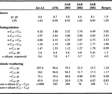
Table 2.3 Summary of diagnostic ratios (source, biodegradation and abiotic) as outlined
in Sections 2.3.1 — 2.3.3 for the fuels shown in the reference chromatograms
(Figure 2.3) of the petroleum products used within the Casey region. Isoprenoid
pristane and phytane are abbreviated to pr and ph respectively 21
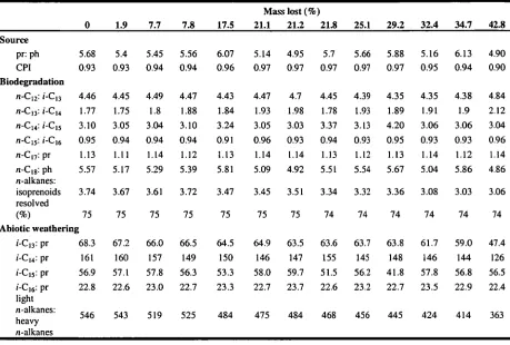
Table 2.4 Summary of the diagnostic ratios in Sections 2.3.1 — 2.3.3 for SAB as it is lost
through evaporation at -20°C. Isoprenoid pristane and phytane abbreviated as pr
and ph respectively. Light n-alkanes: heavy n-alkanes represents the sum of
n-alkanes between n-C
9
—
18:sum of n-C
17and n-C18 25
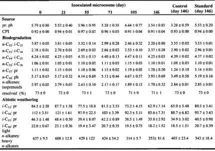
Table 2.5 Summary of diagnostic ratios in Sections 2.3.1 — 2.3.3 for SAB as it is lost
through biodegradation at 4°C. Isoprenoid mistane and phytane abbreviated as pr
and ph respectively. Light n-alkanes: heavy n-alkanes represents the sum of
n-alkanes between n-C9 — n-C18: sum of n-C17 and n-C18 as there was insignificant
quantities of fuel components with ECNs > 18.5 in the neat SAB. 34
Table 2.6 Summary of diagnostic ratios in Sections 2.3.1 — 2.3.3 for neat SAB and the
Table 3.1 Hourly averaged in
situsoil temperatures during summer at Old Casey station,
Antarctica at two sites, a relatively dry and wet site. Maximum and minium
temperatures represent the hourly averaged temperatures. 49
Table 4.1 Microcosm conditions used to test the effects of water and nutrient additions
on the mineralisation of
14
C-octadecane and degradation of the aliphatic
components of SAB at 10°C. Nitrogen concentration was estimated by summing
natural and added N. The C:N ratio was calculated from an initial hydrocarbon
concentration of 15 000 ppm. Repeat microcosm data are from Chapter 3; A
sub-sample of soil I was incubated as part of the previous study for 45 days and a
different sub sample was incubated as part of these experiments for 95 days.
Treatments indicated with an asterisk are shown twice on the table. 62
Table 4.2 Gas chromatography results for pre and post incubation (95 days at 10°C)
microcosm soils. Soil I did not contain squalane and thus these indices can not be
calculated. Results are the average values and is of replicates shown in Table 4.1.
Isoprenoids are abbreviated as pristane, pr; phytane, ph and squalane, sq. 67
Table 4.3 First order mineralisation rate half-lives
T112,and zeroth order mineralisation
rates of
14
C-octadecane to
14
CO2 in soil microcosms at different N loadings
between the time intervals indicated. The lag was estimated from the time delay
required for the best-fit zeroth order function. The microcosms indicated by an
asterisk did not exhibit a plateau phase of
14
C-octadecane mineralisation. At these
concentrations, first order rates were calculated as the average time for the
evolution from 10 % to 100 % of the total
14
CO2. 69
Table 5.1 Results of nonlinear regressions on the production curves for different
temperatures, with ideal linear microbial growth (X = 0) and non-ideal (Gaussian)
mineralisation. So and the root-mean-square regression residual R are expressed in units of mg 14C-octadecane/(kg soil) converted to 14CO2, ico' in units of mmol
14
C-octadecane/(g soil)/day, k2 in units of Cr2, and v in units of days. Confidence
intervals are expressed at the 95% level. 92 Table 5.2 Results of non-linear regressions on the production curves for different
temperatures, with ideal exponential microbial growth (X = 0) and non-ideal
(Gaussian) mineralisation. So and the root-mean-square regression residual R are
expressed in units of mg 14C-octadecane/(kg soil) converted to 14CO2, ko in units of
mmol 14C-octadecane/(g soil)/day, E0 and p in units of d-1 , and v in units of days.
Confidence intervals are expressed at the 95% level. a Estimated value 93
Table 5.3 Temperature dependence of the total 14CO2 production from the highly
bioavailable fraction 98
Table 5.4 Results of nonlinear regression on the production curves for different nutrient
concentrations, with ideal exponential microbial growth (X=350 or 0) and non-ideal
(Gaussian) mineralisation. So are expressed in units of mg "C-octadecane kg soil -1
converted to 14CO2, k, in units of 14C-octadecane kg-soil -1 d-1 , E, and p are in units
of d-1 and v in units of days. 100 Table 6.1 Numbers of heterotrophic and hydrocarbon degrading bacterial numbers as
determined by MPN (cells per g dry soil -1 ). Mean and standard deviation (1s) are
shown. NG is no cells recovered in the MPN medium 114 Table 6.2 Pair-wise ANOSIM of the DGGE banding patterns with initial control and test
soil combined but excluding the 42°C controls. R statistic is a measure of similarity
permutations. Each treatment and control consisted of three replicates, while the
initial soil represents four treatments. Ten and 2.9 % are the best achievable statistic
level with 3 x 3 or 3 x 4 replicates compared respectively.
119
Table 6.3. Whole-cell fatty acid compositions (% of total) of the dominant hydrocarbon
degrading bacteria isolated from each microcosm. Isolates are labelled according to
incubation temperature, microcosm replicate and isolate. All isolates were grown
on TSA Individual fatty acids which comprised less that 0 1% of the totals were
combined into the other acid column, which includes: 12:0, 14:0 30H, i16:1colOc,
17:0, i17:1col lc, a17:1col lc, 17:hol2c
122
Table 6.4. Pair-wise ANOSIM of the isolated FAME composition including FAME
composition of mucoid and non-mucoid isolates from Danne et al. (2002). Groups
indicate the temperature the bacteria were isolated at (or colony morphology). R
statistic is a measure of similarity (0 is maximum similarly while 1 is maximum
dissimilarly) while the significance level is the percent of instances the observed
pattern occurs during random permutations 123
Table 6.5. Pair-wise ANOSIM of the isolated FAME composition including FAME
composition of mucoid and non-mucoid isolates from Danne et al. (2002) grown at
28°C. Groups indicate the temperature the isolates were grown at before
phospholipid extraction. R statistic is a measure of similarity (0 is maximum
similarly while 1 is maximum dissimilarly) while the significance level is the
percent of instances the observed pattern occurs during random permutations 124
Table 7.1 Summary of the chemical treatments applied to the soil from the
semi-enclosed box-plot and open-plot small-scale implementation ICO field trials.
The semi-enclosed box-plot experiment was established in duplicate, composites
samples from 4 separate locations within each plot in the open-plot small-scale
field trial was taken at each time Asterisks indicate where only single samples were
obtained. Treatments were applied in the open-plot small-scale field trial on days 1
and 14. 133
Table 7.2 Soil parameters and chemical results for the open-plot small-scale trial.
Arrows indicate before and after oxidant treatment. Unk represented unknown
values as the samples were lost in transit. Air and soil temperature at time of
samplings varied between -3.8 and -0.5°C and 1.8 and 13°C respectively. 138
Table 7.3 Average results for the geochemical and microbial analysis of the soil from the
semi-enclosed box-plot ICO trial. Pr is pristane. MPNs are in most probable
number of microbes per g dry soil -1 . Percentage hydrocarbon degrading bacteria of
total heterotrophic bacteria are shown in parenthesises in the hydrocarbon
degraders column. Some samples were not collected because the soil was frozen.
ND is Not Detected, detection limit of MPN method was 0.03 x 10 3 microbes g-1 .
Standard deviation (1s) are shown (n=2). Biodegradation data from Snape
et al.(2003) are shown for comparison (n=4). 141
substituted benzenes are tentatively based on literature data (Gustafson
et al.,1997).
14
Figure 2.2 60 MHz- 'H-nuclear magnetic resonance spectrum of neat SAB in
d-chloroform (CDC13), residual CHC13 appears at 7.3 ppm, internal standard (IS) is
tetramethylsilane (Si(CH3)4). Side chains (R) are of undetermined structure 15
Figure 2.3 Reference chromatograms of the main fuels known to have been spilled in the
Casey region (SAB = Special Antarctic Blend, 'Bergen' = arctic blend diesel, MGO
= marine gas oil, Jet-Al = ATK or aviation turbine kerosene). Isoprenoids are
shown by *• An expansion of the n-C 17 — phytane region of each trace is included to
show the relative concentration of these compounds 17
Figure 2.4 Gas chromatography traces of SAB with varying degrees of abiotic weather
(-20°C). Panel A shows the entire envelope of GC-FID detectable compounds
present in neat SAB
(cf.Figure 2.1). Panels B-E are expansions of Panel A; panel B
also shows cyclo-octane which was used as a quality control standard. Methyl- and
ethyl- groups are abbreviated to Me and Et respectively. Structures of the
isoprenoids are shown in Appendix 10.1 24
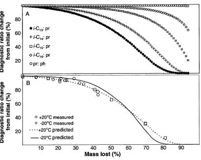
Figure 2.5 Snape
et al.(Submitted) and experimentally derived changes in the abiotic
weathering diagnostic ratios for SAB. Panel A shows the predicted change in the
light to heavy isoprenoid diagnostic ratios and a source (pristane: phytane) ratio.
Panel B is the change in both the experimentally and modelled change in the i-C 13:
pristane ratio at both -20 and 20°C. Isoprenoids pristane and phytane abbreviated to
pr and ph respectively. 26
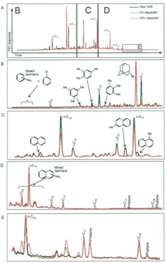
Figure 2.6 Gas chromatography traces of SAB with varying degrees of biodegradation in
liquid-phase microcosms. Panel A shows the entire envelope of GC-FID detectable
compounds present in neat SAB (cf. Figure 2.1). Panels B-E are expansions of
Panel A; panel B also shows adamantane which was used as an internal standard, squalane was also used as an internal standard but is not shown in the figure. Note
the extra peaks in Panel E (red and green lines), these peaks are likely to be polar
compounds, but were not identified. Methyl- and ethyl- groups are abbreviated to Me and Et respectively. Structures of the isoprenoids are shown in Appendix 10.1 32
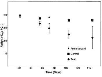
Figure 2.7 Biodegradation diagnostic ratio (n-C12: i-C13) over the 146 days incubation at
4°C. Error bars (1s) are also shown. 33
Figure 2.8 Chromatogram of the fuel contamination at Old Casey Station (Panel A) and
neat SAB (Panel B). Isoprenoids are shown by *• 38
Figure 3.1 Design of the microcosms used in the experiments to measure mineralisation
of 14C-octadecane to 14CO2. 46
Figure 3.2 Recovery of 14CO2 from 14C-octadecane in microcosm experiments. The different symbols identify replicates. The best-fit production curves from the Trefry and Franzmann (2003) (exponential growth rate) are also plotted (see Chapter 5).51
Figure 3.3 Gas chromatography results showing total aliphatic hydrocarbons in the pre-and final microcosm soils in panel A; pre-and percentage change from the pre-treated
soil for n-C17: pristane and n-C 1 8: phytane in panel B. Control data is from the 15°C
microcosms. Error bars (2s) are shown. 54 Figure 4.1 Panel A- percentage of 14C-octadecane mineralised to 14CO2 in Antarctic soils
treated with ca 500 mg N kg-soil-H20 -1 incubated at 10°C for 95 days. The 420 mg
(sterile) control microcosms (closed circle symbols) and unamended controls
(closed square symbols). All symbols represent the average of the number of replicates shown in Table 4.1 and error bars represent Is. Panel B- total aliphatic
hydrocarbon concentration, normalised to squalane, in the pre-treatment, and after
95 days incubation at 10°C for the control and treatment microcosm soils. Points
are an average of data from microcosms in each treatment. Error bars (1s) are shown, data also present in Table 4.2. Panel C- percentage change from
pre-treatment soil of two common biodegradation ratios (n-C17: pristane and n-C18: phytane). Error bars (1s) are shown, data also present in Table 4.2. Panel
D-percentage change from pre-treatment soil of an evaporation ratio (i-C13: squalane). Note that the 420 mg N kg-soil-H20 -1 microcosm data are not present as these microcosms did not contain squalane. Error bars (1s) are shown, data also present
in Table 4.2 68 Figure 5.1 Arrhenius plot of the natural log of the first order rate co-efficient (kJ,
Equation 5.5) for 14CO2 production from 14C-octadecane in the microcosms presented in Chapter 3. Mineralisation rates were calculated from the exponential
phase of growth except for the 28°C microcosms which is shown twice (lag and
exponential mineralisation rates are shown). Microcosms grown from -2 to 28°C
are nominally labelled as psychrotrophic, while mesophilic microcosms are from 28
to 42°C. Error bars (2s) are shown 89
Figure 5.2 Ratkowsky (1983) plot and best-fit estimates when applied to the
"C-octadecane mineralisation rates (-2°C to 28°C) from Chapter 3 90
Figure 5.3 Temperature dependence of the exponential growth rate model parameters.
Figure 5.4 Production rate curves calculated using best-fit parameters for the two growth
models, based on the highly bioavailable fraction of the label
99
Figure 6.1 Total aliphatic hydrocarbon concentration (Panel A) and the change from the
initial (pre-treatment) for both evaporation (Panel B; i-C
1
3: pristane) and
biodegradation (Panel C; n-C17: pristane). Square symbols represent the data from
this experiment; data from Chapter 3 are shown for comparison (diamond
symbols). Error bars in panels A-C represent one standard deviation of the
microcosm replicates at each time point, and the change required for statistical
differences according to student t-test are indicated by a broken line on these
panels 112
Figure 6.2 Photographs of the DGGE gels from the analysis of the triplicate soil
microcosms. The outside lanes (unlabelled) on each gel are a standard DNA control
mix used within our laboratory. The DNA from the initial soil (T
zero
) and after 40
analysis. Panel D is the MDS based the temperature the isolates were incubated at
before FAME analysis 118
Figure 6.4 Panel A shows the similarities between the isolates FAME. The tree was
constructed after square-root Bray-Curtis transformation and cluster analysis (group-average linkages). Temperatures indicated after the isolate designations
specify the temperature at which the isolates were regrown to investigate the effect of temperature on FAME composition. Panel B is a phylogenetic tree based on
partial 16S rRNA gene sequences. Isolates are designated according to incubation
temperature and isolate designation, (e.g. 4°C isolate b is 4(b)). Reference
sequences are shown with GenBank accession numbers. Isolates indicated by an
asterisk were isolated by Daane et al. (2002) and isolates with a cross were from
Antarctica (Christner et al., 2001) 120
Figure 7.1 Photographs of the Casey region and experimental plots. Panel A is the
small-scale open-plot field trial. Plots are 1 high NaH0C1; 2 Control; 3 low NaH0C1; 4 Fentons and 5 H202. Soil for the semi-enclosed box-plot was collected
from the lower right hand corner of the insert (circled) and panel B shows the
semi-enclosed box-plots. 134 Figure 7.2 GC trace of the aliphatic fraction of neat SAB with normal and isoprenoid
alkanes labelled. Insert A and B is the GC trace extracted from the control tins pre and post 15 months respectively. The remain aliphatic contamination 2 years after
treatment with 6.25% NaHOCI and Fentons are shown in Insert C and Insert D respectively. Insert E shows the remaining aliphatic hydrocarbon contamination 15
contamination after 3 years of bioremediation treatment (Snape
et al.,2003).
Acyclic isoprenoids are indicated with an asterisk.
147
Equation 5.1 Brunner and Focht (1984) three-half order linear growth model. 83
Equation 5.2 Brunner and Focht (1984) three-half order exponential growth model 83
Equation 5.3 Trefry and Franzmann (2003) model with linear biomass growth. 84
Equation 5.4 Trefry and Franzmann (2003) model with exponential biomass growth. 84
Equation 5.5 First-order rate kinetics
(ki)86
Equation 5.6 Arrhenius (1889) equation
86
Equation 5.7 Ratkowsky (1983) bacterial growth rate model
87
Acronyms
ATK Aviation Turbine Kerosene
CPI Carbon Preference Index
C:N:P Carbon: Nitrogen: Phosphorous
CRN Control Release Nutrients
DGGE Denaturing Gradient Gel Electrophoresis
ECN Effective Carbon Number
EPA Environmental Protection Agency (USA)
FID Flame Ionisation Detector
GC Gas Chromatography
HP Hewlard Packard
HPLC High Performance Liquid Chromatography
ICO
In situChemical Oxidation
IR Infra Red
'cat
Saturated hydraulic Conductivity
MGO Marine Grade Oil
MPN Most Probable Number
MS Mass Spectrometry
NMR Nuclear Magnetic Resonance
PAH Poly Aromatic Hydrocarbons
Ph Phytane
PHC Petroleum Hydrocarbons
PD Photo Ionisation Detector
Pr Pristane
Pearson product moment correlation coefficient
SAB Special Antarctic Blend
TCE Trichloroethylene
TLC Thin Layer Chromatography
TPH Total Petroleum Hydrocarbon
Tmax
Maximum growth temperature
Tmin
Minimum growth temperature
Topt Optimum growth temperature
TSB Tryptone Soya Broth
T112
Half life
Sq Squalane
Chapter 1
Petroleum products in Antarctica
1.1 Introduction
The Antarctic can no longer be considered a pristine environment as contamination
from waste disposal sites and petroleum spills has affected many terrestrial and coastal marine areas. Of all the different types of contamination reported on the continent,
petroleum has been identified as one of the most significant problems (Snape et al., 2000). Once a spill has occurred it is particularly problematic to recover or remediate, as many techniques employed in temperate regions are either unsuitable or difficult to
implement in Antarctica. Moreover, the environmental impacts of contamination in Antarctica are also likely to be more detrimental than elsewhere because of the relative
rarity of ice free Antarctic coastal habitats, the slow rates of chemical breakdown and ecological recovery from perturbation, and the wilderness values that may be
compromised (Manzoni, 1992; Gore et al., 1999; Poland et al., 2004).
The 'do nothing' or natural attenuation approach to remediation of petroleum contaminated soils in Antarctica is not effective, with numerous sites still highly contaminated many years after spills have occurred. Therefore, active remediation will
need to be undertaken, provided cost-effective management options can be identified. A number of remediation strategies have been considered for petroleum spills in
Antarctica, but bioremediation has been proposed as the only viable management option that can be implemented on a large scale (Snape et al., 2001). On a smaller scale, in situ
chemical oxidation (ICO) has been identified as a complementary remediation strategy that could deliver fast-acting results for highly contaminated soils and avoid many of the
Bioremediation of petroleum-contaminated soils requires an understanding of the
processes that limit degradation, especially in remote cold regions where operational costs are high and site conditions are very different to those found in temperate and
tropical regions. Although many full-scale bioremediation applications have been
undertaken for petroleum spills in the Arctic, trials in Antarctica have been limited to small-scale controlled-spill experiments (Kerry, 1993; Delille, 2000). Little or no
remediation work has been undertaken on contaminated sites in Antarctica using indigenous microbial communities in weathered spills in which the petroleum
contamination still resides long after the initial period of downward migration and evaporation.
1.2 History of petroleum spills in Antarctica
Perhaps the most famous fuel spill in Antarctica was the Bahia Paraiso incident, in which an Argentine tourist ship sank near Palmer station in 1982 releasing more than 680 000 L of diesel into Arthur Harbour (Karl, 1989; Willcniss and Chiang, 1990;
Kennicutt II et al., 1991; Karl, 1992). Marine spills of this type are often highly visible and are regarded as being ecologically most damaging because their impact is immediate
at many trophic levels (Kennicutt II, 1990). However, many substantial spills also occur on land where the immediate environmental impacts are often not so apparent. For example, 760 000 L of fuel was spilled at McMurdo Station between 1980 and 1989,
with a further 380 000 L spilled at the runway area in three separate incidents (Tumeo and Wolk, 1994). There is a similar unfortunate history of accidental spills around
Australia's Casey Station, with 38 000 L spilled in the 1980s (Reid, 1999); 91 000 L in 1990 (ANARE news, 1990), 16 000 L in 1991 (Melick, 1991) and between 2000 and
into porous soils or dispersed along impermeable frozen ground or ice before passing
through catchments into the near-shore marine environment. Of the 73 reported
petroleum spill incidents recorded by COMNAP in 1999, 59 spills were on land
(COMNAP, 1999). Many of these petroleum plumes will continue to slowly migrate for
decades after the initial accident, often releasing a pulse of contaminants each season
with the summer snowmelt (Tumeo and Cummings, 1996; Snape
etal.,2001).
Given the high frequency and large volumes of petroleum products spilt into the
fragile Antarctic environment, it is perhaps surprising that very little remedial action has
occurred. In response to the ratification of the Madrid Protocol in 1998, the Australian
Antarctic Division instigated a multidisciplinary investigation into the origin,
distribution and fate of contaminants at its stations and bases in Antarctica (Snape
et al.,2001). Of the many potentially contaminated sites identified in the Casey region, two
sites were identified as a priority for remediation based on contaminant loading and the
potential for ecological damage associated with persistent discharge into the near-shore
marine ecosystem. The highest priority is the Thala Valley tip site, which is
contaminated with high levels of cadmium, copper, lead and zinc, and is currently the
focus of a major clean-up effort. The second highest priority is the site of the former
workshop-powerhouse at Old Casey Station, which has very high levels of diesel-range
petroleum hydrocarbons (Snape
etal.,2001; Snape
etal.,Submitted). This study focuses
on the workshop-powerhouse contaminated site and is an integral part of Australian
Antarctic Divisions' investigation into the contaminated sites in the Casey region.
1.3 Old Casey Station and surrounds
Antarctica, Old Casey Station is located on a coastal ice-free rock and gravel peninsula. Sea ice is usually present in the winter months but melts or is blown out each summer
(Snape
et al.,
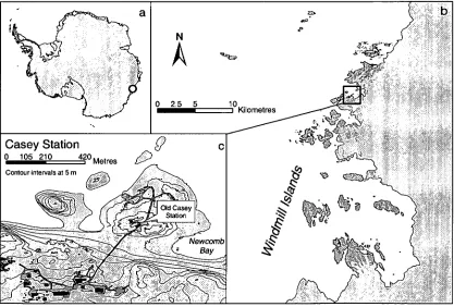
2001). Mean annual air temperature is —9.3°C, with summer air temperatures slightly above freezing, and winter temperatures averaging about —20°C. Mean wind speed averages are about 18 and 31 km hi-4 for summer and winter [image:31.565.116.533.284.566.2]respectively. Annual precipitation is about 180 mm and occurs mostly as snow (Shepherd, 1999).
Figure 1.1 Panel a is a map of Antarctica with the Windmill Islands indicated by a circle. Panel b is a more detailed map or the Windmill Islands region and Panel c shows the location of both the New and Old Casey Stations.
The Casey region contains some of the most developed and extensive flora
communities on continental Antarctica and thus several areas have been designated as Sites of Special Interest (ATCM, 1985). This region has unusually extensive bryophyte
conditions (Smith, 1990). The nearby marine ecosystem is also diverse and shallow waters, away from the impacts of abandoned waste sites and petroleum spills, support
communities of algae, invertebrates and fish. The Windmill Islands are also breeding
grounds for seals, penguins and flying birds.
1.4 Physical characterisation of the Casey region
The distribution and nature of soils is highly variable on local scales of tens to hundreds of metres. Loamy fine earth is separated from sand, gravel and larger clasts by
extensive cryoturbation (Blume et al., 1997). However, soil development is generally poor in the immediate vicinity of the station and has been extensively modified by human activities. In particular, many areas have been covered in coarse aggregate, and
nearby accumulation of fine-gained soils deposited by runoff and wind deposition is common. Organic matter in the soils is initially derived from either dead moss (Beyer et
al., 1995) or more locally through the input of penguin guano (Beyer et al., 1997). Carbon (C) concentrations vary from <0.5 - 10 wt %, total nitrogen (N) is relatively
high, typically <0.3 wt % and C:N ratios are generally low, with C:N generally <30, possibly indicating high availability of humic matter. Availability of micronutrients, such as phosphate (P) and potassium (K), is also considered to be relatively high (Beyer
and Bolter, 1998).
Soil moisture is highly variable laterally, vertically and seasonally. During the winter
months there is no free water or associated runoff. As the summer thaw progresses, snow melt initially ponds within the snow profile or more commonly at the interface
between snow and the frozen active layer. The first melt pulse then disperses largely by
The locus of this movement tends to occur at the base of the advancing active layer and
soil moisture gradients can develop between only a few weight percent soil-moisture
near the surface down to saturation and about 40-50 % water by weight, just above the
base of the active layer. In detail, however, the soil water regime around Casey is highly site dependant.
1.5 The Old Casey petroleum plume
The contaminated site selected for this study was from a large spill that accumulated
in front of the mechanical workshop-powerhouse at Old Casey Station. This site, used for parking and as a refuelling area for station vehicles, was subjected to chronic
small-scale contamination while the station was operational (1969-1989). The most extensive contamination occurred in 1988 when approximately 38 000 L of Special
Antarctic Blend (SAB) was spilled (Reid, 1999). Unfortunately, there are no official records of the spill or the action taken in response to the spill, but the site was
recognised as being highly contaminated by Deprez et al. (1994) in their 1993-94 survey of the region. Deprez et al. (1994) identified an old plume that contained total petroleum
hydrocarbon (TPH) concentrations > 10 000 mg kg-1 in several samples, and one sample with 47 631 mg TPH kg -1 . The workshop-powerhouse site is denoted by Deprez et al. (1994) as WS6 and WS7. Snape et al. (2001) also described the petroleum
contamination at this site, noting that some intrinsic remediation has taken place.
The workshop-powerhouse is located on a rocky promontory 18 m above sea level.
Petroleum-contaminated soils occur throughout the catchment from the site of the old powerhouse, down gradient through to Newcomb Bay. Soils at the spill site are mostly
Soil in the immediate study area consists of fluvial modified glacial deposits that are
equally well described as mineral sediments (Snape et al., 2001). The main spill zone comprises poorly developed soil and an aggregate road. Relatively undegraded SAB still
leaches into Newcomb Bay during the annual summer melt (Revill et al., 1998). The site
is locally heterogenous in terms of contaminant concentration, grain size and wetness (Revill et al., 1998). Because of the high contaminant concentration, and its relatively
fast flow rate into the near-shore marine ecosystem, soils in the vicinity of the Old Casey Station workshop-powerhouse have been identified as a priority for remedial clean-up (Snape etal., 2001).
1.6 Objectives and thesis outline
The overall objective of this study was to evaluate in situ bioremediation and ICO as remediation options for the contaminated soils at Old Casey Station, with the hope of
using research from this site as a case study to be applied to other contaminated sites throughout Antarctica and other cold regions. The general approach adopted in this
study is similar to many other treatability studies. Typically, a treatability study first consists of site and spill characterization, primarily to identify to what extent natural attenuation processes have degraded the plume (e.g. Yang et al., 1997; Margesin and
Schinner, 2001; Delille and Pelletier, 2002). In such studies, field sites are often characterised by a variety of techniques and methods including photo-ionisation
detection (PD) of the volatile hydrocarbons (e.g. Clark, 2003), soil pH analysis (e.g. Filler and Barnes, 2003; Fiore et al., 2003), gravimetric soil moisture (e.g. Grundy et al.,
1996; Cho et al., 2000), hydraulic conductivity (e.g. White and Williams, 1999) and the
There are a number of possible analytical methods for the investigation of petroleum
hydrocarbon contamination, for example infra-red (IR) spectrophotometry (e.g. EPA method 418.8) and high performance liquid chromatography (HPLC) (e.g. EPA 8325
and ASTM D-6379). However, for diesel range organics, the method of choice is gas
chromatography-flame ionising detector (GC-FTD) as it enables detailed characterisation of constituent components of petroleum products and offers a good comprise between
selectivity, sensitivity and cost (e.g. Wang et al., 1995; Wang and Fingas, 1997; Wang and Fingas, 2003a). The characterisation of the aliphatic fraction of fuels provides evidence of biotic and abiotic mechanisms responsible for hydrocarbon removal which
is discussed in Chapter 2. The unambiguous characterization of evaporation and biodegradation processes based on alkanes within a spill are extremely useful parameters
from which remediation efforts can be gauged (e.g. Bragg et al., 1994; Bonham, 2002;
Prince et al., 2002).
For ICO, the key issues relate to whether the treatment removes the hydrocarbon contamination, and what damage it does to the soil and micro-fauna in the process
(Watts and Dilly, 1996; Zappi et al., 2000; Chen et al., 2001; Yeh et al., 2003). In other assessments of ICO efficacy, contaminant removal was monitored using combined field and laboratory analyses including soil pH and temperature measurement (e.g. Yeh et al.,
2002), PD and GC-FID analyses of the soil contaminant concentration (e.g. Watts et
al., 2000). Damage to the soil microbiota can be assessed with a variety of methods, but the most probable number (MPN) estimations is perhaps the simplest measure of
microbial community health (discussed in Chapter 7).
To quantify biodegradation in the soil through successive manipulations, radiometric
constraining rate processes (e.g. Whyte
et al.,1999; Mohn and Stewart, 2000; Whyte
etal.,
2001). For any biodegradation treatability study, the main objective is to quantify the
rate of biodegradation under various environmental restraints which can be precisely
controlled. By isolating the effects of one variable, it is possible to establish what the
limitations of bioremediation are and how these restraints can be favourably managed.
Previous investigations into temperature, nutrients and water have used soil from the
Arctic and Sub-Antarctic regions, which have fundamentally different physical and
biological characteristics and are under contrasting climatic conditions (e.g. Loynachan,
1978; Walworth
et al.,1997; Macnaughton
et al.,1999; Mohn and Stewart, 2000; Brook
et al.,
2001; Eriksson
et al.,2001). The effects of temperature (Chapter 3), nutrients and
water (Chapter 4) on biodegradation of petroleum hydrocarbons in Antarctic
contaminated soils are investigated in this study.
Empirical fitting of the microcosm mineralisation results, such as from Chapter 3 and
Chapter 4, to the various kinetic models provides useful estimates of the dependence of
key microbial population parameters (Arrhenius, 1889; Ratkowsky
et al.,1983; Brunner
and Focht, 1984; Trefry and Franzmann, 2003). The availability of these functions raises
the possibility of applying the radio-isotope mineralisation curves to obtain quantitative
estimates of
in situremediation efficiencies under the seasonal thermal cycles and
nutrient concentration manipulations at Old Casey Station.
electrophoresis (DGGE) (Powell et al., 2003), phospholipid fatty acids composition
(Nichols et al., 1986) microarrays (Zhou, 2003), functional gene expression (Watanabe and Hamamura, 2003), and stable isotope (Pelz et al., 2001; Manefield et al., 2002;
Pombo et al., 2002; Adamczyk et al., 2003). No one technique allows for the identification and characterisation of the key microbial elements within a contaminated
site; scientists are reliant on a combination of culture-dependent, molecular, chemical and physiological approaches. To gain an insight into the population dynamics within
microcosm studies and to determine the bacteria responsible for petroleum-hydrocarbon degradation under psychrotrophic and mesophilic conditions, soil microbial populations
were characterised by MPN estimation of heterotrophic and hydrocarbon degrading bacteria, microbial communities where characterised by denaturing gradient gel
electrophoresis, and individual cultures of numerically-dominant hydrocarbon degrading bacteria were characterised by 16S rRNA gene sequencing and fatty acid methyl ester
(FAME) analysis.
Ultimately, no single technique can provide an unequivocal measure of all the processes occurring in contaminated soil undergoing remediation, and the results of
Chapter 2
Characterisation of the petroleum hydrocarbon contaminants
at Old Casey Station
2.1 Introduction
There are numerous techniques and analytical procedures used in the characterisation
of crude oil and its' refined products. The concentration of total petroleum hydrocarbons (TPH) in environmental samples can be determined by non-specific methods such as
infra-red (IR) spectrophotometry (EPA method 418.8, Table 2.1) or gravimetrically (EPA method 9071B, Anon, 2003). Detailed characterisation of the individual components of petroleum occurred as early as 1857 with the identification of several
aromatic hydrocarbons (Speight, 2001 and references therein). More recently, detailed characterisation of petroleum hydrocarbons is usually performed with chromatography
methods. There is an extensive choice of analytical methods including, but not restricted too, gas chromatography-flame ionization detection (GC-F1D) (eg. EPA method 8015B
(Anon, 2003)), GC mass spectrophotometry (MS) (eg. EPA method 8270C and ASTM D-2425 (Nadkarni, 2000)), photo ionization detection (PID) (eg. EPA method 8021B),
high performance liquid chromatography (HPLC) (eg. EPA 8325; ASTM D-6379), thin layer chromatography (TLC) (eg. Cavanagh et al., 1995; Watson et al., 2002), supercritical fluid chromatography (SFC) (eg. EPA 3560) and nuclear magnetic
resonance (NMR) (eg. ASTM 5292).
The choice of an analytical procedure is largely determined by factors such as speed,
selectivity, sensitivity, cost and the objective of the analysis. In environmental matrices,
constitutes, and also the characterisation of the biomarkers used to indicate the source,
[image:39.564.95.522.201.547.2]nature and type of spilt petroleum products.
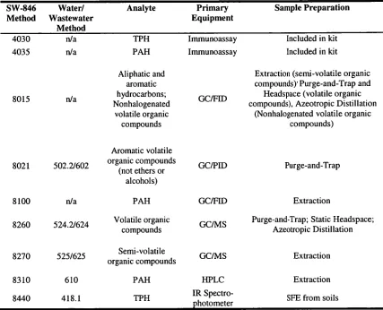
Table 2.1 U.S. Environmental Protection Agency (EPA) test methods for determining petroleum hydrocarbons (reproduced from Anon, 1997). Numbers refer to EPA method numbers. Several types of analyses do not have established water/ wastewater methods (n/a — not available).
SW-846 Method
Water/ Wastewater
Method
Analyte Primary Equipment Sample Preparation 4030 4035 8015 8021 8100 8260 8270 8310 8440 n/a n/a n/a 502.2/602 n/a 524.2/624 525/625 610 418.1 TPH PAH Aliphatic and aromatic hydrocarbons; Nonhalogenated volatile organic compounds Aromatic volatile organic compounds
(not ethers or alcohols) PAH Volatile organic compounds Semi-volatile organic compounds PAH TPH Immunoassay Immunoassay GC/FID GC/PID GC/F1D GC/MS GC/MS HPLC
IR Spectro- photometer
Included in kit Included in kit
Extraction (semi-volatile organic compounds)' Purge-and-Trap and
Headspace (volatile organic compounds), Azeotropic Distillation
(Nonhalogenated volatile organic compounds)
Purge-and-Trap
Extraction
Purge-and-Trap; Static Headspace; Azeotropic Distillation
Extraction
Extraction
SFE from soils
2.2 Petroleum products at Australian Antarctic Stations
A wide variety of petroleum products have been used at the Australian Antarctic Stations, including mineral and synthetic lubrication oil, marine gas oil (MOO), light
diesel, kerosene, and petrol. The most common product used by Australia is MGO, a
heavy marine diesel, although this is largely limited to use on resupply ships. The most commonly used product on the continent is a light diesel fuel, Special Antarctic Blend
and heavy vehicle transport. Aviation turbine kerosene (ATK) and petrol are used to a
much lesser extent for helicopters, light aircraft and for vehicles that travel off station to
the interior of the continent.
As most refined petroleum products are manufactured for performance rather than for specific composition, some degree of compositional variation (Appendix 10.2) within
one product is likely and is influenced by the availability and composition of the parent material (Gill and Robotham, 1989). The chemical compositions detailed below are
based on samples obtained from the manufacturer in 2002-03.
SAB is specially refined by BP Australia for use in cold climates and a summary of
the historical chemical composition as supplied from BP is shown in Appendix 10.2. SAB is the main soil contaminant at Old Casey Station, and thus it has been
characterised in more detail than the other petroleum products used by the Australian Antarctic Program. While there is batch to batch variability, generally SAB is primarily
comprised of aliphatic hydrocarbons with n-alkanes in the range nonane (n-C9) to tricosane (n-C23) with concentrations peaking around dodecane (n-C12) (Figure 2.1). It also contains several acyclic isoprenoids, such as those shown in Appendix 10.1. Figure
2.1 shows the differences in neat SAB when the aromatic hydrocarbons are removed with silica-alumina chromatographic cleanup (Section 3.2.4). Silica-alumina cleanup
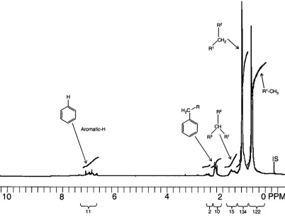
removes up to ca 19% of the total hydrocarbons. 'H-NMR analysis of neat SAB
indicates that only ca 4% of the protons are bound directly to an aromatic ring (Figure
2.2). Biomarkers such as the pentacyclic hopanes and the C27 to C29 steranes, having effective carbon numbers (ECN) >27 (Gustafson et al., 1997), can not be detected in significant quantities in SAB by GC-FID analysis. Fresh SAB has a relatively high
proportion of resolved compounds, with a resolved proportion from n-C9 to hexadecane
0. Ce 0 a 1 13 Total SAB Aliphatic fraction -■■ n-Ca
n-C1, i .
Time
Me Me
Mixed
QMe,
isomers me X>
4.
6
•
z
(
L e za.v. .j..4. Me i(e)
Me I
SMAAOArao
4/ %/IN.c269.69N.AAA.
1n -C1 2
Me CO
L=0:&-kA
C5-
4
I n-C 13
Co
Me
l
e1/4-1-...
Mixed ixed
isomers me, 9 w i w w 2.- a) c
(-1) —
c c 0 . 9 E c CL
-..
Figure 2.1 Gas chromatography traces of the total and aliphatic fractions of SAB. Panel A shows the entire trace. Panels B-E are detailed locations of Panel A. Identification of the naphthalene, 1-methyl, 2-methyl naphthalene and the di-methyl naphthalene hydrocarbons were by spikes of known structures. Identification of the substituted benzenes are tentatively based on literature data (Gustafson etal., 1997).
1111111111111111111111111111111111111111IIIIII
10 8 6 4 2 OPPM
[image:42.565.72.474.56.366.2]11 Lr21
16
j
15 134 122Figure 2.2 60 MHz- 'II-nuclear magnetic resonance spectrum of neat SAB in d-chloroform (CDCI3), residual CHCI3 appears at 7.3 ppm, internal standard (IS) is tetramethylsilane (Si(CH3)4). Side chains (R) are of undetermined structure.
Both ATK and Jet-Al have very similar aliphatic component as SAB (Figure 2.3); they are slightly more volatile peaking at undecane (n-CI I). The resolved component of
these fuels is ca 75% (Table 2.2). While MGO also peaks at n-C11, it has a higher
concentration of the heavier alkanes and is the heaviest fuel used by the Australian Antarctic Program. The resolved component of MGO is similar to SAB, with a resolved
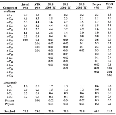
Table 2.2 Resolved components of the diesel-ranged fuels commonly used by the Australian Antarctic Program.
Jet-Al ATK SAB SAB SAB Bergen MGO Component (%) (%) 2003 (%) 2002 (%) 2002 (%) (%) (%)
n-alkanes
n-C9 2.0 1.5 0.1 0.2 0.2 0.3 1.3
n-C10 4.6 3.7 1.8 2.3 2.1 1.1 3.0
n-C11 5.3 4.4 3.6 4.7 3.5 1.7 3.6
n-C12 4.4 3.6 4.4 4.8 4.8 1.8 3.1
n-C 13 2.8 2.6 4.4 3.7 4.9 1.6 2.2
n-C14 1.1 1.6 2.8 1.4 3.0 1.0 1.4
n-C15 0.2 0.4 0.4 0.1 0.8 0.8 0.8
n-C16 0.02 0.1 0.03 0.05 0.3 0.6 0.7
n-C17 0.01 0.02 0.05 0.1 0.5 0.7
n-C18 0.01 0.01 0.04 0.1 0.3 0.6
n-C19 0.01 0.01 0.04 0.02 0.3 0.6
n-C20 0.01 0.03 0.2 0.5
n-C21 0.01 0.02 0.1 0.4
n-C22 0.01 0.02 0.1 0.2
n-C23 0.01 0.01 0.02 0.1
n-C24 0.01 0.01 0.05
n-C25 0.01 0.02
n-C26
isoprenoids
i-C13 1.0 0.9 1.2 1.3 1.1 0.6
0.01
0.6
i-C14 0.9 0.9 1.5 1.2 1.2 0.6 1.3
i-C15 0.3 0.4 0.6 0.3 0.6 0.3 0.3
i-C16 0.2 0.3 0.3 0.1 0.5 0.4 0.4
Pristane 0.01 0.02 0.04 0.07 0.5 0.5
Phytane 0.01 0.01 0.01 0.2 0.1
Resolved 75.3 73.6 70.0 71.0 72.8 64.9 71.3
Arctic blend diesel obtained from Bergen, Norway has occasionally been used as an alternative to SAB (Figure 2.3). While the aliphatic fraction of 'Bergen' fuel also peaks
at n-C12, the same as SAB, the fuel is slightly heavier than SAB as it contains higher concentrations of the alkanes from tetradecane (n-C14) to docosane (n-C22). 'Bergen'
fuel has the least resolved component of the diesel-range fuel used by the Australian
FID
response
— n-C,
7
pristane
K
PhYtane
0 0
n-C n C n-C,0 n-C,, n-C12 n-C,
3
n-C,
4
n-C,
3
n-C16 n-C,
7
n-C,
8
n-C,
3
n-C
23
n-C2, n-C
22
n-C23 n-C
24
Jet-Al = ATK or aviation turbine kerosene). Isoprenoids are shown by *• An expansion of the n-C17 region (SAB = Special A ntarctic Blend, ' Bergen' = arctic blend diesel, MGO = marine gas oil,
2.3 Precedence for use of diagnostic ratios
GC-FID analysis of petroleum hydrocarbons offers a good comprise between selectivity, sensitivity and cost; although a more detailed characterisation of the
constituents of petroleum requires GC-MS. Analysis of contaminated soils and waters by GC-FID and GC-MS provides a fingerprint of the petroleum hydrocarbons present.
Hydrocarbon fingerprints can be useful for identifying the source of petroleum hydrocarbons in the environment and monitoring its subsequent breakdown. At the
simplest level, TPH analysis can be used to measure concentrations and monitor decreases with time. One of the problems with TPH measurements is that many of the compounds found in petroleum hydrocarbons either occur naturally in the environment or fractionate on a GC at the same time as natural organic material, and it is sometimes difficult to assess at a spill site how much of the petroleum is anthropogenic (e.g.
Woolard et al., 1999; Wang and Fingas, 2003b). It is also difficult to assess how much petroleum has migrated vertically or laterally from the site, how much has been diluted,
or how much has been lost through evaporation or biodegradation. More detailed fingerprinting techniques aim to identify and quantify a range of organic compounds.
These can be used to define source signatures, differentiate between contaminant sources that might have similar chain length molecules, and provide estimates of changes associated with dilution, evaporation or biodegradation (e.g. Gill and
Robotham, 1989; Wigger and Torkelson, 1997; Whittaker et al., 1999; Wang and Fingas, 2003b). The differentiation of biotic (e.g. biodegradation) and abiotic (e.g.
volatilisation) weathering processes, determining the biodegradability of any spilled
Of the numerous diagnostic ratios outlined in the literature (e.g. Humphrey et al.,
1987; Wang et al., 1995; Wang and Fingas, 2003a), very few can be used at the Old Casey Station contaminated site. Typical ratios often utilise hopanoid compounds, such
as C30-17a(H),2113(H)-hopane (ECN ca 27) (Bence et al., 1996); SAB generally contains insignificant concentration of any compounds with ECNs >20.
Of the ratios identified in the literature the following can be used at the Old Casey
Station contaminated site to identify the source of the petroleum contamination (Section 2.3.1), the degree of biological (Section 2.3.2) and abiotic (Section 2.3.3) loss of the
light diesel products used by the Australian Antarctic Program.
2.3.1 Source identification
• Pristane: phytane (Gill and Robotham, 1989; Wang et al., 1998 and references therein)
• Heptadecane (n-C17): pristane (Wang et al., 1999)
• Carbon preference index (CPI), ratio of odd-carbon n-alkanes: even-carbon n-alkanes, used to identify biogenic or petrogenic hydrocarbons — biogenic
n-alkanes tend to have odd number of carbon atoms (Boehm et al., 1987; Humphrey et al., 1987; Gill and Robotham, 1989 and references therein)
2.3.2 Biodegradation
• n-alkane: matching isoprenoid such as (n-C17: pristane and octadecane (n-C18): phytane) (Boehm et al., 1987; Wang and Fingas, 1997; Wang et al.,