Scattering of a Rayleigh Wave by the Edge of a Thin Surface Layer

SCATTERING OF A RAYLEIGH WAVE BY THE EDGE OF A THIN SURFACE LAYER

Thesis by

Donald Alan Simons

In Partial Fulfillment of the Requirements For the Degree of

Doctor of Philosophy

California Institute of Technology Pasadena, California

1975

Acknowledgments

The author wishes to express his sincere appreciation to

Professor J. K. Knowles for his invaluable guidance during the course of this work.

The work was performed with the support of Hughes Aircraft Company through its Howard Hughes Doctoral Fellowship Program. The author is deeply appreciative of this support.

In addition, partial support was provided by the Institute under its Graduate Teaching Assistantship and Fellowship programs, and by the Office of Naval Research under Contract N00014-67 -A

Abstract

This investigation treats the problem of the scattering of a Rayleigh wave by the edge of a thin layer which covers half the surface of an elastic half-space. The interaction between the layer and the half-space is described approximately by means of a model in which the effect of the layer is represented by a pair of boundary conditions at the surface of the half-space. Two parameters- one representing mass and the other, stiffness- are found to characterize the layer.

The incident Rayleigh wave impinges normally upon the plated region from the unplated side.

In the case where the mass of the layer vanishes, the problem is solved exactly using Fourier transforms and the Wiener-Hop£

technique, and numerical results are obtained for the amplitudes of the reflected and transmitted surface waves. In the more general case of a layer possessing both mass and stiffness, a perturbation procedure leads to a sequence of problems, each of which may be

Table of Contents

Introduction 1

l. Pure Surface Waves 6

2. Formulation of the Problem 15

3. Solution for a Massless Layer 21

4. Approximate Solution for a Very Thin Layer.

39

5. Conclusions and Comments 51

>:<

Appendix A - Roots of R (x.) 52

Appendix B - Factorization of D(x.); Properties and

Evaluation of D+(x.) and D-(x.) 58 Appendix C - Certain Aspects of the Solution in the 66

Case of a Massless Layer

[image:5.564.73.474.106.403.2]

List of Figures

Figure 1.

Figure 2. Figure 3.

Figure 4. Figure 5.

Figure

6.

Figure 7.

Figure 8. Figure

9.

Coordinates for a Half-Space Covered by a Thin Layer.

Differential Element of the Surface Layer. Coordinates for a Half-Space Cove red by a

Semi-Infinite Thin Layer. Complex x.- Plane.

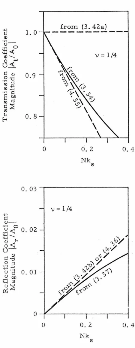
Transmission and Reflection Coefficients for the Case of a Massless Layer.

Approximate Transmission and Reflection Coefficients for the Case of a Very Thin Layer. Com,flex x.-Plane for Determination of Zeros

of R (x.).

*

Complex R -Plane.

Complex a-Plane for Evaluation of D+(x.).

7

10

16

25

37

50

53

Introduction

The present work is concerned with the scattering of an

elastic surface wave by the edge of a thin surface layer.

The principal motivation for studying the relation between

elastic surface waves and thin surface films comes from the field of

microwave signal processing. Electromagnetic waves may be

con-verted to elastic waves in solids, and vice versa, by means of

piezo-electric transducers. Operations such as delaying and filtering of

signals may be performed on the elastic waves by suitably designed

devices [ 1] 1. The advantage of carrying out such operations in the

elastic- rather than the electromagnetic- medium comes about

primarily from the fact that the phase velocities of elastic waves are

typically five orders of magnitude smaller than those of

electro-magnetic waves [ 2]. Thus, for example, the length of delay line

required for a given delay is smaller, by this ratio of phase

veloc-ities, for an elastic wave than for an electromagnetic wave.

Elastic surface waves prove to be more advantageous than

body waves because of their accessibility. Thus, for example,

sur-face wave delay lines may be built with numerous taps along the way,

providing incrementally varying delays.

The surface of an elastic solid acts in a sense as a waveguide,

i.e. , energy once transferred into surface waves tends to remain in

fields concentrated near the surface. For purposes of microwave

Reference [ 1] provides a general survey of the design and function

signal processing it is also desirable to confine- or guide- elastic

fields laterally. The basic premise in designing "surface waveguides"

is that a strip of the surface on which the characteristic surface wave

velocity is lower than that of the surroundings will tend to guide

sur-face waves along its length. This is sometimes implemented by

depositing a thin layer of a heavy, soft material on the surface in the

form of a strip. The thin layer ''loads" the substrate, creating a

zone in which the surface wave velocity is lower than that in the

unplated region. Conversely, on a surface fully plated with a light,

stiff material except for a strip that is left unplated, the strip again

acts as a guide since the surface wave velocity is higher in the coated

. [ 2] 1. reg1on

Straight surface waveguides of the type described above have

been analyzed by Tiers ten [ 3], who represents the effect of the

sur-face layer by a boundary condition at the surface of an isotropic

substrate. He derives from his model an equation for the velocity of

the "straight-crested" (i.e., plane strain) surface waves

character-istic of the plated region. He then appeals to a concept introduced by

Knowles [4] to demonstrate the existence- in the same plated

region- of a more general class of surface waves referred to as

"variable-crested" surface waves. The full field in the substrate is

synthesized approximately from the variable- ere sted surface waves

characteristic of the plated and unplated regions, by applying an

approximate m atching condition at the boundary between the regions,

and by requiring the surface waves outside the strip to decay

exponen-tially along the surface away from the strip. This leads to an

approxi-mate dispersion relation for the guide, i.e. , an equation relating the

frequency and velocity of disturbances propagating along the guide.

Tiers ten and Davis [ 5] have extended this analysis to the case of a

curved surface waveguide.

Freund [6] has treated a structure similar to that treated in

[3] using a more exact approach. The surface of the guiding strip

considered in [6] is assumed to be traction-free, while the surface

outside the guide is assumed to be free of shear stress and to suffer

no vertical displacement. The scattering of a single straight-crested

surface wave incident on the edge of a semi-infinite guide at

arbi-trary angle is solved exactly. An approximation to the dispersion

relation for a guide of finite width is obtained by superposing incident

and reflected straight-crested surface waves and neglecting at one

edge of the guide the body waves generated at the other edge. Fossum

and Freund [7] have obtained and solved the dispersion equation for

the guide by an independent method based on an integral equation, and

thereby have validated Freund's original approach.

Apart from the problem solved by Freund in [6] as an

inter-mediate step in his analysis, there are no known exact solutions for

scattering of an elastic surface wave by the edge of a surface layer.

Approximate solutions employing juxtaposition of straight-crested

surface wave modes have been obtained by Li et al [8] and McGarr

In contrast, exact solutions do exist for the scattering of

cer-tain types of electromagnetic surface waves. Of particular interest

is the work of Kay [10], who considers the scattering of an

electro-magnetic surface wave by a discontinuity in a property of the surface

known as normal impedance. An exact solution is obtained by using

the Wiener-Hop£ technique. The problem is closely analogous to the

present one, and in fact has served as a "proving ground" for some of

the techniques employed here.

To complete this brief summary of related literature, note

should be taken of the study of Koiter [ 11] of the static problem of

load transfer from a stringer into a plate. The problem is one of

generalized plane stress, but is essentially identical to that of a

half- space in plane strain, half of whose surface is plated with a thin

layer, with a static line load acting on the edge of the layer and

paral-lel to the surface. The effect on the substrate of the stiffness of the

layer is modeled in precisely the same manner as in the present

analysis.

Although the present consideration of the scattering of a

sur-face wave by a thin layer was motivated by the signal-processing

applications discussed above, the results of the analysis may also be

of interest in connection with seismology.

This study begins in Section 1 with a review of pure surface

waves in half-spaces with the surface either fully traction-free or

fully covered with a thin layer. In Section 2 the central problem is

-6-l. Pure Surface Waves

For the purposes of this study, a pure surface wave is a

solu-tion of the elastodynamic equasolu-tions of mosolu-tion in a half- space which

propagates in a direction parallel to the surface and decays

exponen-tially with depth. Such waves can exist in a half space with the

sur-face either fully traction-free or fully covered by a layer of a

differ-ent elastic material. In this section the properties of pure surface

waves are reviewed, with emphasis upon a method of approximating

the effect of a surface layer in the case where the layer is thin. It is

necessary to understand these waves before the problem

correspond-ing to the scattercorrespond-ing of a surface wave can be formulated.

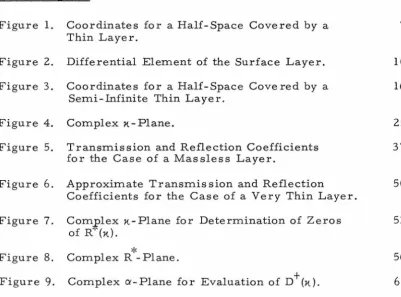
Consider a half- space occupied by an elastic, isotropic,

homo-geneous solid with Lame parameters

A.

and ~ and density p, covered

by a layer of thickness 2h' of a different material with Lam~

param-eters

A.'

and ~' and density p'. A coordinate system is established

as shown in Fig. 1, with a y-axis running out of the plane of the

paper. The displacements in the x-, y-, and z-directions in the

half-space are denoted by U, V, and W respectively, and in their

fullest generality are functions of x, y, z, and time t. The case of

plane strain is assumed, so that all displacements are independent of

y, and V

=

0. Further, the time dependence is assumed to be

har-monic with

-iwt U(x, z, t)

=

u(x, z)e ,

w

>0

.l

( l. 1) -iwt

A.',fJ', p' 0

A.,IJ.,p

[image:12.563.128.471.266.530.2]

z

Figure

1.

Coordinates for a Half-Space Covered by a Thin Layer.

-8-For convenience, the amplitudes u, w will henceforth be referred to

as displacements. Since actual, physical displacements must be

real, those corresponding to the present problem are either the real

or imaginary parts of the quantities appearing in (1. 1).

Under the foregoing assumptions the elastodynamic equations

of motion will be satisfied if the displacements are related to the

two-dimensional Lame' potentials iii (x, z), 'Y(x, z) by1

u(x, z)

( l. 2)

w(x, z)

and if the potentials satisfy the reduced wave equations

2

2

'V iji +kd iji

=

0 '

,..,2,u+k2w _{V I S I}

=

0 _{, - 00 <X< 00 , Z;;:: ,} 0

where

( l. 3)

The potentials iJi and '¥ are referred to respectively as the dilatation

and shear potentials; the speeds cd and cs are respectively the

dila-tation- and shear-wave speeds.

2

The stresses are related to the potentials by the formulas

1see[l2]

2 2 82 82'¥ 0 = _{11 [} (2kdk + 2

-2) iJi -2~ ],

XX S

8X uxuz

82iJi 2 82 0xz = 1J[2n--a- (k + 2 - ) '¥],

uxuz s ₈z2

0

zz

( l. 4)

The pure surface waves of interest here are solutions of (1. 3)

which decay exponentially with z and satisfy appropriate conditions at

z

=

0. Such solutions take the form

iJi(x, z)

=

Ae -nd(k)z±ikx,

'" ( _{r x, z -}) _ AP. _1-'e -n (k)z±ikx _{s , ( l. 5)}

where

n (k)

=

Jk

2 -k2 ' k>k , p

=

d, s,

p p' p

and where A, (3, and the wave number k are constants yet to be

deter-mined.

Now assume that the layer covering the half- space is thin

enough that the displacements within the layer can be taken

approxi-mately as independent of z. By virtue of the requirement that

dis-placements be continous across the interface between the layer and

the half-space, the displacements in the layer must then coincide with

those in the half-space at z

=

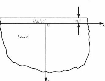
0.

Consider the forces acting on a differential element of the layer

of unit width in the y-direction and of length dx, as shown in Fig. 2.

Upon neglecting all internal stress resultants in the layer except those

due to simple stretching, the balance of momentum in the x- and

-,dxr-.,+ ___

2_h_'cr_n_

D

2h '( (J n

+ :

(J p_ dx)

Zh' ... X ----~~X X

t

!

..

cr xz (x, O)dx cr (x, O) dx

zz

z

Figure 2. Differential Element of The Surface Layer .

[image:15.566.131.453.201.543.2]

oa

2hl J. ( ) 1 I 2

a-+a

_{ux xz} x,O +2hpw u(x,O)=O,l

a

(x, 0) + 2h1

p\iw(x, 0) = 0, zz

( l. 6)

where

a;

is the axial stress in the layer. The stresses

a

(x, 0) and xz

a

(x, O) are those exerted by the substrate on the layer. The axial zz

stress

a;

is related to the displacement u(x, 0) by

I( ) -4 I(

A

1+U1) ou(x, 0) ~ x - u X~2u'

ox

Substitution of ( l. 7) into ( l. 6) yields

where

2

-o

u(x 0)

a

(x, O) +uN

i

+uMu(x, O) = 0,

xz

o

x

a

(x, 0) +uMw(x, 0) = 0, zz

8hl I 11+ I 2hlpiW2 N -~ ( fl. bl ) M- =~-...;,;._.,

- u "-'+2u' ' - u

( 1. 8)

Note that N and M are measures of the layer's stiffness and mass,

respectively.

Equations (1. 8) may be thought of as boundary conditions to be

satisfied by the fields in the substrate. Note that in the absence of a

covering layer, M = N = 0 and ( 1. 8) reduce to the boundary conditions

appropriate to a traction-free surface. Tiers ten [3] deduced ( l. 8)

from a more general development in which Mindlin's plate equations

[ 13] were taken as a starting point2. He argued that for thin plates

1 This relationship is derived from the three -dimensional stress- strain law under the assumption of plane strain in the y-direction and vanish-ing of normal stress in the z-direction.

all terms except those involving axial stretching and inertial reaction

are negligible.

Substitution of the potentials (l. 5) into (l. 2) and (l. 4), and

thence into the boundary conditions (l. 8), yields a pair of

homage-neous, linear, algebraic equations in

A

and

A!3.

The condition for

the existence of a non-trivial solution is that the determinant of the

coefficient matrix vanish. This is

R(k)- Nk2k2n (k) + M[k2[n (k) + nd(k)]

s s s s

2 2 2 2

+Nk [k - ns(k)nd(k)]}+M [ns(k)nd(k)- k } = 0 ( l. 9)

where

2 2 2 2

R(k) = (2k - k ) - 4k n (k)nd(k)

s s (l. 10)

Each value of k satisfying ( 1. 9) determines an elastic surface

wave through ( l. 5), provided k>k (note that k > kd' provided A> 0

s s

and ~ > 0 - see (

l.

3)) and provided

!3

has the now common value

re-quired by either of the boundary conditions (1.8). If the time

depen-dence is restored in the potentials (l. 5), their x- and t-dependence,

and hence that of all field quantities, is of the form

±ikx- iwt ±ik(x :ret)

e

=

e (l. 11)

where c=w /k. Thus the surface wave ( l. 5), while decaying

exponen-tially with z, propagates unchanged in form with speed c in the

positive or negative x-direction according to whether the positive or

negative sign is used in (

l.

ll ).

If the surface layer thickness 2h' vanishes, M=N=O, the

R(k)

=

0 . ( l. l 2)

Equation (l. 12) determines the propagation speed of Rayleigh waves,

an extensive discussion of which may be found on pp. 307- 309 of

Love's text [15]. Achenbach, on p. 190 of [16], proves that there is

only one root of (l. 12) greater than ks. This root is denoted by kR

and referred to as the Rayleigh root or the Rayleigh wavenumber. If

(l. 12) is multiplied by w -4 the resulting equation for cR

=

w/kR, and

hence cR itself, is independent of w. The Rayleigh wave is thus said

to be non-dispersive, i.e., its propagation speed cR is independent of

frequency w.

In the more general case Eq. (l. 9) may have one or two

roots [3]. The smaller one, which will be denoted kT and referred

to as the extended Rayleigh root, reduces continuously to kR as M and

N go to zero, while the other root goes to infinity in this limit. If

N ~ 0 or M

f:.

0, the speed corresponding to the extended Rayleigh root

is frequency-dependent, so the presence of the layer results in

sur-face waves which are dispersive.

A special case of interest is that of a massless layer, for which,

by (1.8), M=O, and (1.9) reduces to

>:< 2 2

R {k) = R(k) - Nk k n {k) = 0

s s (l. 13)

It is shown in Appendix A that this equation also has but one

admissi-ble root. This root is less than kR' reduces continuously to kR as

N .... 0, and corresponds to a dispersive surface wave which propagates

in keeping with the intuitive expectation that a stiffening layer would increase the characteristic surface wave speed.

It must be noted that if the sole objective of the present paper were a study of pure surface waves, it would not be necessary to make

2. Formulation of the Problem

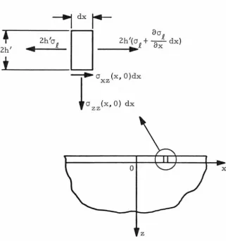
An elastic, isotropic, homogeneous solid occupies the half-space -ro<x, y<oo, z~O . A thin layer covers and is bonded to the surface z

=

0, -ro<y<ro, x>O, as shown in Fig. 3. Notations for coordinates, material properties, and field quantities are exactly as in the previous section. The assumptions of plane strain and harmonic

-iwt

time dependence of the form e are maintained, so that the problem may be formulated in terms of the time-independent Lam~ potentials

<t> (x, z), 'f(x, z). The reduced wave equations governing these

paten-tials are (1. 3), the displacement-potential relations are (1. 2), and the stress-potential relations are (1. 4). The boundary conditions for the unplated surface are

a

(x, 0)

=

0

-oo<x<O

.1

zz

( 2. 1)

a

(x, O)

=

0

xz

and for the plated surface, in accordance with the assumptions and results of the previous section,

a

(x, 0)

+

f..LMw(x, O) =

zz

0 ,

1

a

2u(x 0)

a (x, 0)

+

f..LN

z'

+

f..LMu(x, 0)

=

0 , O<x<ro .

xz

ox

(2. 2)

The potentials 4>, 'f are required to be twice-continuously differentiable in the interior of the half-space. The quantities appear-ing in the boundary conditions (2. 1), (2. 2) are required to be continu-ous up to the respectively appropriate segment of the boundary, ex

-cepting the origin x

=

z

=

0 . Certain further conditions, which will be

-16-AI I I

, ~ , p

0

/..,~,p

z

Figure 3. Coordinates for a Half-Space Covered

by a Semi-Infinite Thin Layer.

[image:21.563.125.445.88.496.2]

various field quantities as the origin is approached, these conditions

having the effect of ruling out point loads and higher-order

singulari-ties at the origin.

The potentials <ii, '¥ are required to be of the form

<ii (x, z) = A₀cpR + (x, z)H( -x) + ArcpR- (x, z)H( -x)

+AtcpT+(x, z)H(x) +cp(x, z),

'i'(x, z)

=

A

01jTR+(x, z)H(-x) + ArljiR- (x, z)H(-x)

+ AtljTT+(x, z)H(x) + ljl(x, z) .

( 2. 3)

In Eq. (2. 3), cpR±, ljiR±, cpT+, and ljiT+ are normalized potentials

representing positive- and negative -traveling Rayleigh waves and the

positive-traveling extended Rayleigh wave corresponding to the layer,

and are given by

where

=

-nd(kR)z ± 2kRx ,1,

=

±~ -n (kR)z±ikRx

cpR± e , "'R± ~"R e s ,

i3R

=

2ikR ns (kR) '

2 2

2kT-ks -~Mnd(kT)

f3T

=

2ikTns

(kT)-i~MkT

(2. 4)

The constant A

0 is given, the constants Ar and At are unknown,

H(x) is the unit step function, and cp and 1jT are required to satisfy the

radiation conditions

ik r e s

ljl(x, z)""'G(8)

J? ,

-18-t 2 21

-1

uniformly in 8 for 0S:8$1T . Here r:::: 'Vx +z ,

8

::::Tan (z /x), as r-+oo,

F(8) and G(8) are unknown functions of 8, and the symbol

"rv"

denotes asymptotic equality in the usual sense.

The motivation behind (2. 4) will be discus sed presently, but

first a matrix notation will be introduced which not only simplifies

some of the subsequent manipulations, but consolidates the

fundamen-tal concepts of the analysis. Twice-underlined letters will denote

2

x

2 matrices of partial differential operators, and underlined letters

will denote column vectors with two components, the first of which is

a dilatational potential, and the second, the corresponding shear

potential. Thus the reduced wave equations ( l. 3) become

where

L::::

L iJi:::: 0

-~

:::: lip

(x, z)

'!'(x, z)

The boundary conditions (2. l) and (2. 2) become

where

R iJi :::: 0, z :::: 0, -oo<x<O,

= - -

-(R

+

N~

+

MT

)_! ::::

0 , z :::: 0 , 0 <x<oo ,

R::::

0 0

S::::

03

a3

-2

ax az

a2

2

-axaz

a

T::::

-

a a

( 2. 6)

The required form of the solution (2. 3) becomes

where

.P_R±=

(2. 8)

ikTx

e ,

l

cp(x,

z)l ,

~(x,z)

and where cp(x, z) and ~(x, z) must satisfy the radiation conditions (2. 5).

Now it can be seen that in the assumed form (2. 8) each of the first three terms represents a surface wave propagating in either the positive or negative x-direction and existing only for either positive or negative x. The first term is the incident wave and has amplitude A

0 . The remaining terms taken together constitute the scattered wave and propagate outward from the origin. These terms are

referred to respectively as the reflected wave, the transmitted wave, and the radiated wave; the ratios Ar/ A

0 and A/ A0 are referred to respectively as the reflection and transmission coefficients.

is separated into various parts, some representing surface waves,

3. Solution for a Massless Layer

It is now assumed that the layer's density p' vanishes.

According to (1. 8), this causes M to vanish. Under this condition the

governing differential equations (2. 6) remain the same, but the

bound-ary conditions (2. 7) reduce to

R ! =

Q,

z = 0, -oo<x<O,

(R + NS)ili = 0, z = 0, O<x<oo

=

::::::::~-

-

.}

(3. 1)

The assumed form (2. 8) and the radiation conditions (2. 5) remain, but

the wave number kT appearing in (2. 8) is now a root of the simplified

form (1. 13) of the more general dispersion relation (1. 9).

The order conditions at the origin are taken as

0 (x,O)=O(l), xz

80 (x, 0)

+

xz

ox

-pl

= O(x ) as x ... 0 , p1 <1 , (3. 2)

The solution to the problem specified by (2. 6), (3. 1), (2. 8),

(2. 5) and (3. 2) will be obtained in closed form in this section.

It is convenient to define a new function ~(x, z) by

A

,!(x, z) = A

0cpR+(x, z) +~(x, z) . (3. 3)

Recall that A

0 is the amplitude of the incident Rayleigh wave. Thus A

for x<O,

2

comprises the scattered wave, while for x> 0 it consists

of the scattered wave minus a positive-traveling Rayleigh wave of

A

amplitude A

0. In either case,

.:£.

consists only of

A

The differential equations governing T_ are obtained by

substi-tuting (3. 3) into (2.

6),

and by noting that, according to (1. 3) and (2.

6),

L T_R

+

=

Q.

This yields A

L T_

=

Q ,

-co <x <co , z:?: 0 • (3. 4)

A

The boundary conditions for cp are obtained by substituting (3. 3) into

(3. 1), and by noting that, according to (1. 8), (1. 2), (1. 4) and (2. 7),

R cpR+

=

Q.

This yields

A

R T_

=

Q ,

z

=

0 , -co <x <co ,

A

AONik;kR {0} ik

X

(R

+

N~)5£

=

2 e R , z

=

0 ,

- - 1

O<x<oo,

l

(3. 5)

where use has been made of the definition of S in (2. 7) and that of

13R

in (2. 4).

This problem will be solved with the aid of a Fourier

trans-form on x. Let f(x) be a complex-valued, absolutely integrable

func-tion of the real variable x which satisfies

(3. 6)

for some positive constants K,

o

and

x

0. The exponential Fourier

transform of f(x) is defined by

co

"'

_{f (x.)}

=

J -

_f(x)e ix.x _{dx, -o <Irn x. <o ,} [ } _{(3. 7)}

-co

and the inversion formula is

co

1

J"'

i~x

f(x)

=

21T f (x.)e · drt, -co<x<co . (3. 8) -co

transform f(x.) is analytic in the domain - o <hn [x.} <o (see [ 20],

p. 338).

It is clear from (2. 8) that for fixed z the potentials P, '1' will

not satisfy the decay condition (3. 6) for any o>O, as long as the wave

numbers kR'· kT, ks and kd are real. However, application of the

Wiener-Hop£ technique (which will be explained presently) requires

that the transforms be analytic in strips of the complex x.-plane such

as that defined in (3. 7). The difficulty is resolved by temporarily

assuming that the frequency

w

has a small, positive, imaginary part,

while all propagation speeds remain real. This is a standard artifice;

it is discussed, for example, on p. 28 of [ 21 ]. After the solution is

obtained, the imaginary part of w will be taken to vanish.

Now since ~ is required to contain only outwardly propagating

waves, the assumption that hn

fw}

> 0 (and consequently that

hn[kQ'} >0, Q'

=

d, s, T, R) renders

i

exponentially decaying in lxl as

required by (3. 6), with decay constant 6 satisfying O<o<hn[kd}

(c£. (3. 3), (2. 8), (2. 5)).

Formal application of the transform (3. 7) to the differential

equations (2. 6) yields

(3. 10)

2'">:'

a

'l'(x., z)- 2( );;( )

2- n x. r x., z

=

oz

s

0 , -o <hn [ x.} <6,

where

1 2 21

n =Vx. -k

The functions ns (x.) and nd(x.) are rendered single-valued in the entire rt-plane and analytic in the strip -o<Irn[rt}<o by taking branch cuts as shown in Fig. 4, and by requiring ns (rt) and nd(x.) to approach

+oo as x. ... oo along the positive real x.-axis. The solutions of (3. 10) are then

~(x.,

z)

=

A(rt)e -nd(x.)z + A'(x.)end(x.)z,

l

r (

1{ ' z ) = B ( 1{. ) e - n s ( 1{. ) z + B I ( 1{.) ens ( 1{. ) z ' -0 <Irn [ 1{. } < 0 '

(3. 11)

where A(x.), A'(x.), B(x.), and B'(x.) are unknown functions of x.. How-ever, the coefficients A'(rt) and B'(x.) must vanish; otherwise the transforms would grow exponentially with lx.l for z>O, and the inver-sion integrals (3. 8) would not converge. This leaves

'i::' ~(x.,z)

~(x.,

z)

=

A(rt)e -nd(rt)z,

I

= B (x.) e-ns ( x.) z , -6 <lrn [ x.} <

o

.

(3. 12)

The boundary condition (3. 5), when written in component form, becomes

2

2 ....

( 2k2 - k2 + 2-8

-)cr

+

2~

=

o,

z

=

o,

-oo<x<oo,

d s

az2

axaz

(3. l3a)

(3. 13 b)

0

-k R

-k s

Im[;~t}

B_

[image:30.566.69.517.104.709.2]

-26-fact that the mass of the layer is neglected at present, so that M

=

0 1n

(2. 2). In contrast, the conditions (3. 13b, c), which relate to the

normal tractions at z = 0, take different forms according as x<O or

x> 0. The fact that only one of the boundary conditions changes form

at x

=

0 makes possible the application of the Wiener-Hop£ procedure

in its simplest form.

It is now convenient to define functions f(x) and g(x) on (0, co)

and (-co, 0), respectively, by setting

(3. 14)

Apart from a factor ~. f(x) and g(x) are the unknown values of 0 and xz

2 2

0 +~No u/Elx under the layer z = 0, O<x<oo, and on the free sur-xz

face -oo<x<O, z

=

0, respectively.

Formal application of the transform (3. 7) to (3. 13) and {3. 14),

followed by use of (3. 12), yields

(2x. 2- k2)A(x.) - 2ix.n (x.) B(x.)

=

0,

s s

2 2

-- 2ix.n (x.)A(x.)-- {2x. -- k )B(x.)

=

F (x.),

s s

where

(X)

I

-htx F- (x.)

=

f(x)e dx,

0

0

G+(f(.)

=

Jg(x)e-ix.xdx.

-(X)

(3. 16)

The functions f(x) and g(x) as defined by (3. 14) are

exponen-tially decaying for large positive and negative x, repsectively, with

-

+

decay constant 6. Moreover, since F (x.) and G (x.) are half-range

transforms of f(x) and g(x), F- (x.) and G+ (x.) are analytic functions

of x. on the half-planes Imfx.} <6 and Im[x.}

>

-6, respectively (see

p. 12of[21]). The superscripts on F (x.) and G (x.) are thus seen

-

+

to be suggestive of the half-planes on which the functions are

respec-tively analytic.

After A(x.) and B(x.) are eliminated from (3. 15) there remains

the single equation

where

R(x.)

*

2 2

R (x.)

=

R(x.) - Nk x. n (x.) s s

(3. 17a)

(3. 17b)

It is important to note that the domain of validity of (3. 17a) is the

strip -6 <Im [ x.} <6.

Now define D(f(.) by

D(x.)

=

2(k;-

k~)R*

(x.)

2

'

Nk n (x.)R(x.) s s

It is shown in Appendix B that D(x.) admits the representation

where

D(x.)

=

D- (x.) D+(x.)

OO'FiO

=

exp{--1-.

J

Log[D(ct)]da} -o<Im[x.}<o

2TT1 • J: Q'-1{ '

-<Xl=fl u

(3. 19)

and that D+(x.) and D-(x.), by trivial analytic continuations, have the

scune domains of analyticity as G + (x.) and F- (x.), respectively. In

view of (3. 18) and (3. 19), Eq. (3. 17a) may be rewritten as

2 - -

-Nk n (x.) D (x.)F (x.) s s

The functions n±(x.) are rendered single-s

valued in the entire complex x.-plane and analytic in the strip

-o<Im[x.} < 6 by taking branch cut!:! as shown in Fig. 4, and by

re-quiring both n+(x.) and n-(x.) to approach too as x.-oo along the

posi-s s

tive real axis. Note that the superscripts have the scune meanings as

above.

Equation (3. 20) is said to be of Wiener-Hop£ type. The method

used to solve it is referred to as the Wiener-Hop£ technique, and is

,Im[K}<6,

(3. 21)

The function H+(K), by a trivial analytic continuation, is analytic for Im[K}>-6, while H-(K) is similarly analytic for Im[K1<6. Accord-ing to {3. 20), there is a common strip of analyticity in which

{3.22)

It follows that there is an entire function H(K) such that

(3. 23)

+

Now it will be proved that both H-(K) and H (K) tend to zero as IKI-+oo in the appropriate half-plane. The order conditions {3. 2) imply the existence of positive constants L and E: such that

Ia {x, O)I<L

xz , O<x==::E:,

(3. 24) Ela (x, 0)

I

x:x

I

<Lx -pl ' 0 <x::::E: '

I

a

(x, O)

I

< Ke -ox , E:~x<oo,

xz

(3.25)

8a (x, 0) l'.

I xz Clx I <Ke -vx , E:~x<oo, 2

I

a

_xz

(x,O)+~Na

u(x,O)I<Keox _{2 '}

-oo<x~-E:.

8x

Substitution of (1. 2) and (1. 4) into (3. 14), thence the result into (3. 16), yields

(X)

-

I

-i~x

~F (~)

=

a

(x, O)e dx,

xz (3. 26a)

0

0 2 .

~G+ (~)

=

I

[a

xz (x, 0) +

~N

8

u(~,

0)

J

e

-l~xdx

•

-oo 8x

(3. 26 b)

One integration of (3. 26a) by parts, followed by use of (3. 24) and

(3. 25), leads to the following asymptotic estimates for F-(~) and

G+(~):

a

(x, o) . loo ₁ oor

aa

(x, o) .

I

IIF-(~)1

=

xz l~X + xz -l~Xdx

~ -i~ e o+ i~ oi 8x e

0

(3. 27)

= 0(

~~-l)

as

l~l

.... oo,

Im[~}<o,

0 -8

I~G+ (~)I ~

I

L lxrp2 _{dx +}

IKe

_oxdx

It is proved in Appendix B that

ID+(~)I

....

l

as

1~1-+oo, Imf~}>

-6,}

ID-(~)1-+1 as 1~1-+oo, Imf~}<6.

Use of (3. 27) and (3. 28) in (3. 21) yields

H- ( ~) .... 0 as 1~

1-+ oo ,

Im [

~

}

<

6 ,

+

H (~)-+0 as 1~1-+oo, Im[~}>-6.

(3. 28)

Therefore (3. 23) and a trivial extension of Liouville's theorem (p. 125

of [22]) imply that

H(~)

=

0 . (3. 29)

+

In view of (3. 29), (3. 23), and (3. 21), F-(~) and G (~) are

given by

rm[~}<6,

(3. 30)

Im[~}>-

6.

Substitution from (3. 30) into (3. 15) yields three equations in A(~) and

B(~). Any one of these may be considered as redundant and the

re-maining two solved for A(~) and B(~) to give

A(~) = (3.3la)

B(1-t)

=

(3.3lc)

The alternate forms are obtained by using (3. 18) and (3.19).

yields

Application of the Fourier inversion formula (3. 8) to (3. 12)

00

cp(x, z)

=

2

~

J

A(1-t)e -nd(1-t)z + i1-txd1-t, -00

00

~

(x, z)

=

2~

J

B(1-t)e -ns (1-t)z + i1{xd1-t -00

(3. 32)

as formal candidates for a solution to the original problem for cp, ~. Several steps are now necessary to prove that the functions cp,

$

appearing in (3. 32) are properly defined and actually satisfy (3. 4) and (3. 5). These steps are left to Appendix C. It is also proved there that the asymptotic forms of F-(1-t) and G+(1-t) as j1-tj ... oo are in fact as specified in (3. 27).

In order to demonstrate that (3. 32) contain the surface waves required by (2. 8), the integrals in (3. 32) must be regarded as complex contour integrals along the real 1-t-axis in the complex 1-t-plane (see Fig. 4). The singularities in the integrands in (3. 32) are due to the various singularities of D+(1-t) and D- (1-t), the branch points of n (1-t)

[image:37.560.153.495.66.205.2]

points at -ks and -kd' no zeros, and a simple pole at -kT' while

D- (x.) has branch points at ks and kd, no zeros, and a simple pole at

*

By inspection of (3. 17b) it is seen that R(x.) and R (x.) have

branch points at ± ks and ± kd' and it is proved in Appendix A that

their only zeros are located at ± kR and ± kT, respectively. Hence

the singularities of the integrands in (3. 32) are branch points at ± k

s

and ± kd' and simple poles at ± kR and ± kT. These are shown in

Fig. 4. That they are not on the real axis is due to the assumed small,

positive, imaginary part of

w.

The branch cuts are taken as shown

in Fig. 4. The segments of these cuts between the branch points and

the imaginary axis will lie along the real axis in the limit as Im

[w} ...

0.

Now consider an integration around the closed contour formed by

the quarter-circular arcs of radius R and the appropriate segments

of the branch-line contour and the real axis, as shown in Fig. 4. If

the integrals over the quarter-circular arcs vanish in the limit as

R ... oo, then by Cauchy1 _{s theorem the integral over the real axis may}

be replaced by that over the branch-line contour plus the contribution

from the residues at the poles kT and kR. It can easily be shown

that this is in fact the case when x>O. The residues are evaluated

using (3. 3la, c) and (3. 32). With the aid of (3. 17b) and (3. 3) it is

seen that the contribution due to the pole at kR is equal to the

inci-dent wave AO~R+(x, z) but for its sign. Thus substitution of the

where

-34-<.P (x, z)

=

AtcpT+(x, z) + cp(x, z),

l

'Y(x, z)

=

AtiJ!T+(x, z) + IJ!(x, z), x>O,

A

=

t

,r,. I

R'

'

(kT)

cp(x, z)

IJ!(x,z) =

=

=

-

·-,

dR~-dtt 1{ = k

T

2~

J

A(tt)e -nd(tt)z + ittxdtt'

x>OJ

B+

_1_

J

B( ) -n (tt)z + ittxd

2rr tt e s tt '

B+

(3. 33)

(3. 3 4)

(3. 3 5)

and where B+ denotes the branch-line contour in the upper half-plane

(see Fig. 4). The full field is thus seen to have the required form

(2. 8) for x> 0, with At as the amplitude of the transmitted wave,

pro-vided

cp

and 1J! satisfy the radiation conditions (2. 5). That they do may

be proved by analyzing the asymptotic behavior for large Jx2+z21 of

the integrals in (3. 35). When z

=

0, such an analysis may be carried

out with the aid of Watson's lemma, and when z

f:

0, by the saddle

point method.

When x<O, a similar procedure applied in the lower half of the

tt-plane leads to the result

where

A = r

2 2

+

+

AOkR (ks- kd)D (kR)ns (- kR)

n: (kR)D- (- kR)R'(- kR)

=

d){

dRI

,

1-t =-kR

cp(x, z}

=

2~

I

A(7-t)e -nd(ft)z

+

iftxdft, B

~

(x, z)

=

2~

I

B(7-t)e -ns (7-t)z

+

i){xdft, B_

(3. 37)

x<OJ

(3. 38)

and where B denotes the branch-line contour in the lower half-plane.

Thus the full field has the required form for x<O, with A as the

r

amplitude of the reflected wave.

Note that the functions cp(x, z), ~(x, z) as defined by (3. 35) and

(3. 38) are discontinuous across x = 0, z> 0, but the full field

.!

is

twice-continuously differentiable in the interior of the half-space.

Also note that had (3. 32} been derived formally without

recourse to the assumption of complex frequency, the inversion

con-tour would appear to pass directly through the poles and branch points

(since they would now lie on the real 7-t-axis), and it would be

neces-sary to appeal to some other argument to determine whether this

contour should be considered as passing above, below, or through

these singularities. The assumption of complex frequency, in

addi-tion to providing the overlapping domains of analyticity required for

the Wiener-Hop£ analysis, serves in effect to resolve this dilemma.

-36-It is now desired to obtain numerical values for the reflection

and transmission coefficients Ar

I

A

0, A/ A0. All quantities in (3. 34) and (3. 37) can be evaluated straightforwardly except for the functions

+

-D and D . It is proved in Appendix B that

(3. 39)

so for the purpose of determining Ar/ A

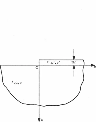
0 and At/ A0 from (3. 34) and (3. 37), it is only necessary to compute D+(kR) and D+(kT). This is done by a numerical integration, the details of which are explained in Appendix B. After rewriting (3. 34) and (3. 37) in dimensionless form it is seen that the coefficients Ar

I

A

0, At/ A0 are functions only of the dimensionless layer parameter Nk and Poisson's ratio

v.

The

s

dependence on Nk of the transmission and reflection coefficients is s

shown for v= 1/4 in Fig. 5. The coefficients Ar/A

0 and At/A0 are complex, but for the range of Nk shown the imaginary parts never

s

exceed 0. 4o/o of the corresponding real part. A complex coefficient simply signifies a wave whose phase is shifted with respect to the incident wave.

A check of these numerical results may be obtained by com-puting, from (3. 34) and (3. 37), the asymptotic forms of Ar/A

0 and A/ A

0 as N-+ 0. The wave number kT is a function of N defined im pli c i tl y by ( 1. 1 3 ) :

1:l

1. 0

<!)

...

_u -... 0

:::::~

< ! )

-0 ....,

u~

!=: <!)

.s

'1J (/) ::s (/) ."",::!

... !=:

s

bO (/) ell

@~

H E-i

0.9

0.8

0. 03 0

0

from {3. 42a)

\) =

1/4

0.2

Nk

s

0.2

Nk

s

\) =

1/4

0.4

0.4

Figure 5. Transmission and Reflection Coefficients

[image:42.560.135.360.80.657.2]

-38-Upon setting N=O, and noting from (1.13) and (1.12) that kT(O) =kR'

there results

Thus

It is proved in Appendix B that for k>k s

Applicationof(3. 39)-(3. 41) to (3. 34) and (3. 37) yields

At = A

0

+

o ( 1 ) ,

(3. 40)

(3. 41)

(3. 42a)

(3. 42b)

The first terms of (3. 42a) and (3. 42b) are plotted in Fig. 5 and it is

clear that they do agree with the numerical computation with

increas-ing accuracy as N-+ 0. Equation (3. 42a) expresses nothing more than

the fact that the amplitude of the transmitted wave approaches that of

4. Approximate Solution for a Very Thin Layer

It is now assumed that the layer is thin enough, when com-pared with the wavelength of any of the characteristic surface or body waves, that the layer parameters M and N, defined by (1. 8), may be taken as perturbation parameters in a sense to be described pres-ently.

so that

Let a constant ex be defined by

p I W 2 (

A/

+

2 ')

a =

""V

X'+

~t;

,

M=aN.

( 4. 1)

(4. 2)

The perturbation process consists of allowing the layer thickness 2 h' to grow from zero to some small, non-zero value while holding ex fixed. Thus, in view of (1. 8), (4. 1), and (4. 2), the problem may be expressed in terms of the single perturbation parameter N.

The differential equation (2. 6) for _!(x, z) remains. By using (4. 2), the boundary conditions (2. 7) may be rewritten as

~!

=.Q.,

z

=

0, -oo<x<O, }

[ R

+

N (~

+

aT )1

!

=

.Q ,

z

=

0 , 0 <x <oo

(4. 3)

-

-

-The assumed form (2. 8) also remains appropriate, with the wave number kT a root of (1. 9), but now it is assumed that the amplitudes Ar' At appearing in (2. 8) may be represented by

A = A(O)+N A(l)+ o(N)

r r r ' }

A= A(O)+NA(l)+o(N) as N ... O,

t t t

and that the radiated wave

cp

may be expressed as

:£(x,z)

=

:e_(O)(x,z)+Ncp(l)(x,z)+o(N) as N-oO (4. 5)

Each term on the right of (4. 5) is assumed separately to satisfy the

radiation condition (2. 5).

The remainder of this section is concerned with the

determi-. (m) (m)

nahon of Ar , At , m

=

0, 1 The first step is to derive the

equa-tions governing

~(O)

and .:r_(l). By substitution of (2. 8) into (2. 6) and

(4. 3), there results the following problem for

2£.:

L

~

=

Q ,

z

>

0 , - ro <x <ro , x

~

0 } R :£

=

0 , z

=

0 , - ro <x <0 , '

{ R + N

(g

+ a T) } ~

=

0 , z

=

0 , 0 <x <ro .

( 4. 6)

The requirement that

!

be twice-continuously differentiable, when

applied to (2. 8), leads to the jump conditions

[T]- Ao'£R+ (0, z)- ArTRJO, z) + AtTTt (0, z)

=

0,}

[2£,

x] - 1kRAO.:P_R+(O, z) + 1kRAr

cpR-

(0, z) (4. 7)

+

ikTAt~T+(O, z)

=

Q,

O<z<ro,

where

J

+

-[cp

=

:£(0 , z)-:£(0 , z) .

When (4. 2) is substituted into ( 1. 9), there results an equation

which defines kT implicitly as a function of N. By differentiating

Equation (4. 8), and the fact that kT = kR when N = 0, lead to

kT = kR +

Nk~l)+o(N)

as N-+0. (4. 9)

The quantity ~T+(O, z), defined by (2. 8), may similarly be

expanded in a power series in N, resulting in

cpT+(O,z)

=.:f:R+(O,z)+N~~l(O,z)+o(N)

as N-+0, (4. 10)

where

N=O

Now (4. 4), (4. 5), (4.

9),

and (4. 10) are substituted into (4. 6)

and (4. 7), and the coefficients of the zeroth and first powers of N in

each equation are separately set equal to zero, to yield

L~(O)=Q,

z> 0, -oo<x<oo, X;{: 0;

R

~(0)

= Q, z = 0, -oo<x<oo, X

F

0;

(0) (0) (O) _

L

~

( 1 ) =

Q ,

z > 0 , - oo <x <oo , x f. 0 ;

R~(

1

)=..Q.,

z=O, -oo<x<O;

R

~

( 1 ) = -

(~

+ a T)

~

( 0) , z = 0 , 0 <x <oo ;

[ r()(1 )J -A( 1)cp (O z)+A( 1 )cp (O )+A(O)cp( 1)(0 ) =_0,

::t:. r - R- ' t -R

+ '

z t - T

+ '

z [cp(l)]+ik A(l)cp (O z)+ik A(l)cp (0 z)

-'x R r -R- ' R t -R+ '

+ ik A(O)cp(l) (0 z)+ik(l)A(O)r() (0 z) = 0 z>O

R t -T+ ' T t .!:.Rt ' - ' ·

( 4. 12)

In order to solve (4. 11), it is convenient to define an

auxil-iary function

~(O)

by

cP(O) = cp(O)- A

cp

H(x) +A (O)cp H( -x) + A(O)cp H(x)

- - 0-R+ r -R- t -R+ ( 4. 13)

When (4. 13) is substituted into (4. 11), the equations governing cP(O)

are found to be

A(O)

L ~ =

Q,

z>O, -oo<x<oo, } R

~(O)

= 0, z = 0, -oo<x<oo, [cP(O)J = [cP(,O)J = 0, z>O.

- - X

-(4. 14)

In particular, note that the differential equation for cP(O) holds

throughout the interior of the half- space. From (4. 13) it is seen that

~(O)

is everywhere outwardly propagating. This fact together with

(4. 14) implies that T(O)

=

Q.

Thus, from (4. 13),

cp(O) = (A -A (O))

cp

H(x)- A (O)cp H( -x)

- 0 t -R+ r -R- ( 4. 15)

A (O)

=

A A (O} - 0 }

t 0' r - '

(0)

T_

(x, z)

=

0 .

( 4. 16)

Equations (4. 16) simply express the fact that in the limit as the

layer vanishes, the full field

!

consists only of a positive-traveling

Rayleigh wave of amplitude A 0.

In view of (4. 16), Eqs. (4. 12) become

L

5£

(

1) =

Q ,

z

>

0 , -co <x <co , x -/: 0 ;

R

T_(

1) =

Q,

z = 0 , -co <x<co , x -/: 0;

(4. 17)

The solution of (4. 17) is facilitated by the introduction of an

auxiliary function

~(

1) defined by

"(1)

When (4. 18) is substituted into (4. 17), the equations for~

found to be

A k(l)

"( 1} _ 0 T { -ik

x}

R~ - ZkR R cpR+(O, z}e R H(-x)

{ ( 1) ik

X}

_

+ A

0 R _T.T+(O, z)e R H(x}, z- 0, -co<x<co,

( 4. 18)

are

(4. 19a)

(4. 19c)

As in the case of .P_(O), the function p_(l) is smooth enough that the

differential equation (4. 19a) holds throughout the interior of the

half-space.

The right-hand sides of (4. 19a, b) may be simplified

some-what. Note that

ik X

3:T+(x, z) = 3:T+(O, z)e T

= [ 3:R+ (0, z) + N

.'£~~

(0, z) + O(N2)] e ikRx [1 +iNk¥ )x + O(N2

)J

lr()(l) ik X . (1)

J

2

= cpR++N[!=-T+(O,z)e R +tkTx~R+ +O(N )asN ... O. (4.20)

Since L ~T+(x, z)

=

Q, each term of the latter form of (4. 20), when

operated upon by L, must vanish. Thus

[-11) ik x

1

_

.

(1) [ }

L pT+(O, z)e R _- -1kT L xcpR+(x, z) ( 4. 21)

From (1. 8), (1. 2), (1. 4), (2. 7), and (4. 2) it follows that

( 4. 22)

Substitution of (4. 20) into (4. 22) leads to

2

+ O(N ) = 0 as N ... 0 , z = 0 . ( 4. 23)

Each term of ( 4. 23) must likewise vanish separately, so

[ (1) ik x

1

.

(1) [ }

R :!:T+(O,z)e R =-1kT R x.:!:R+ -(.e_+aT).:!:R+' z=O (4. 24)

The right-hand sides of (4. 21) and (4. 24) may be easily computed by

R 5£R+

=

Q

at z

=

0. The first term in the right-hand side of (4. 19b) may also be computed directly. These results are then incorporated

into (4. 19) to yield

(4. 25a)

where

( 4. 26)

Equations (4. 25) may be solved with the aid of the Fourier

transform (3. 7). It is once again assumed that the frequency

w

has a

small, positive, imaginary part. The transform of (4. 25a) is then

found to be

"'

2 " (1)

a

cp (x., z) 2( )0:'(1)( ) 2 - n x. cp x., z

=

oz

s

2A

0kR k(.i.)e -nd(kR)z i(x.- kR)

2AOkR k(.-i)f3Re-ns (kR)z

i(x.- kR)

z> O, -o<hn{x.}<6 ,

(4. 27)

where 6 is a constant such that 0<6<hn{kd}. The solution of the

homogeneous version of (4. 27) is given in (3. 11), and again A'(x.),

-46-2A

0kR

k~)e-nd(kR)z

i(x.-kR)2(x.+kR)

z

>

0 ' - 6

<Im [

/{. } <

6

( 4. 28)

Application of the transform (3. 7) to the boundary conditions

(4. 25b), followed by use of (4. 28), yields

=

( 4. 2 9)

This is a system of two simultaneous, linear equations in the two

unknowns A(x.), B(x.). It possesses a unique solution provided the

determinant of the coefficient matrix does not vanish. That

determi-nant is found to be -R(x.), where R(x.) is given by (3. l7b) and is

known to vanish only at x.

=

± kR. Since these points lie outside the

domain of validity of (4. 29), A(x.) and B(x.) may be computed

( 4. 3 Oa)

(4.30b)

Equation (4. 30a), for example, may now be used in the inversion

formula

00

cP(l)(x, z)

=

2~

J

~(7t)e-nd(rt)z_

-co

which follows from (3. 8) and (4. 28).

(4. 3 1)

The singularities of the integrand in (4. 31) are branch points

at ±kd' ±ks' and poles at ±kR. The contributions due to the residues

at the poles represent, as in the previous section, the surface waves.

For x> 0 the contour may be closed in the upper half-plane, as shown

in Fig. 4, so in this case it is the pole at kR. which is of interest.

-48-arising from the last term in (4. 31). The residue of each term may

be computed separately. The first, third and fourth terms have

double poles; the second, a simple pole.

The double poles will lead to secular terms, i.e., terms

con-taining x or z as a factor. It will be seen, however, that none of

these terms appears in the asymptotic expansion of

~(l)(x,

z) as

x -t±oo. This is necessary in order that the asymptotic expansion be

valid; otherwise the representation of

!(

1) (x, z) would not be

uni-formly valid in x and the asymptotic expansion could not be justified.

In fact, it is this very requirement which necessitated the seemingly

roundabout formulation employed in this section.

From (4. 18), for x>O,

(1) - A(l) (1)

cp {x, z) - cp {x, z) - At cpR+(x, z)

( 1 )

(1) ik X AOk:T

-A

0cpT+(O,z)e R - 2k cpR+(x,z), x>O. (4.32)

R

When the four residue contributions from

c$(

1) are combined with the latter three terms of (4. 32), there results

where

( 1) I

A

=

t

A 0 R"(kR)k! { 2

J}

___;:. _ __:::..::..._

2

-=- -

kRn (kR) + et [ n (kR) + nd(kR)

2[R'(k )] s s

R

( 4. 3 3)

Note that the secular terms due to the double poles have been

can-celled by each other and by the third term on the right-hand side of

(4. 32). Now since Cj)(l)(x, z) must obey the radiation condition (2. 5),

it cannot contain any surface waves, so from (4. 33) it follows that

(4.35)

The coefficient A( 1) may be determined by a procedure analo-r

gous to that described above, but with the integration contour closed

in the lower half rt-plane. Because A(rt) has only a simple pole at

rt

=

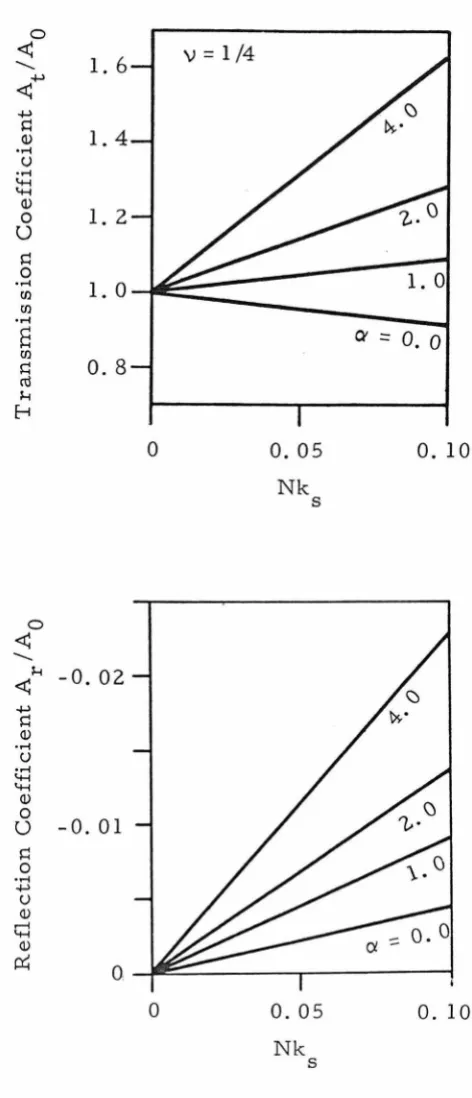
-kR' the computation is somewhat simpler. The final result is

When (4. 16) and (4. 34)- (4. 36) are used in (4. 4), the

trans-mission and reflection coefficients may be computed to first order in

N. The resulting approximations to the coefficients are shown in

Fig. 6 for v

=

1/4.

If the layer is massless, M=O, a=O, and the results may be

compared with those of the previous section. This is done in Fig. 5

[image:55.561.133.369.102.651.2]

0 ~ ..._ ~ ~ ~ 1=1 Q) ... u ... '+-i '+-i Q) 0 0 1=1 0 ... (IJ (IJ

...

s

(IJ

1=1 til l-< f-i 0 ~ ..._ l-< ~ ~ 1=1 Q) ... u ... '+-i '+-i Q) 0 0 1=1 0 ... ~ u Q) ... '+-i Q) r:r::

1.6

v

=

1/4

1.4

1.2

1.0

0.8

0

-0.02

-0.

01

Q

0

-50-0.05

Nk s

0.05

Nk s

Ql :::

o.

₀

0. 10

0. 10

Figure

6.

Approximate Transmis sian and Reflection

5. Conclusions and Comments

The problem of the scattering of a Rayleigh wave by the edge

of a thin surface layer is amenable to solution by the Wiener-Hop£

technique in the case where the density of the layer vanishes. The

amplitudes of the reflected and transmitted surface waves computed

by such an analysis are shown in Fig. 5 for v

=

1

I

4.

A perturbation process leads to an approximate solution for

the case of a layer possessing both mass and stiffness. This analysis

yields the transmission and reflection coefficients shown in Fig. 6,

for v

=

1/4. The results of the two analyses agree closely for very

thin, massless layers.

It is reasonable to ask whether the results of Section 3 might

be extended to the case of a layer having mass, by treating the

layer's mass parameter M as a perturbation parameter, while

allowing the stiffness parameter N to remain arbitrary. Such a

pro-cess leads to a sequence of problems, the zeroth order problem

being precisely that solved in Section 3. This procedure has been

attempted, but the computations required to obtain the first order

solution were found to be of prohibitive complexity. Part of the

diffi-culty arises from the fact that the zeroth-order solution, which is

known only as a Fourier inversion integral, appears as a forcing

function in the first-order problem. This necessitates the

.,,

Appendix A - Roots of R,,,{l-t)

In this section the roots in a suitably cut complex plane of

the function

(Al)

are located.

It is assumed that w

=

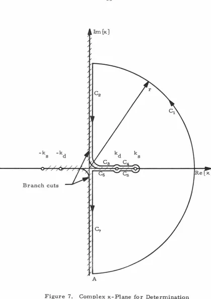
0, so that ks and kd are real. The

branch cuts in the complex x.-plane are taken as shown in Fig. 7,

except that the radii of the cuts in the vicinity of the origin is

vanish-ingly small. The functions ns(x.) and nd(x.) are then defined by

requiring that they be positive for x.>ks. When ns(x.) and nd(x.) are

pontinued analytically throughout the cut 11.-plane, it can be seen that

>!:: >::: ~:<

f-

(x.) is even in 11., i.e., R (11.)

=

R (-x.). Therefore it is only

neces-sary to consider the right half-plane Re[x.}:::: 0.

The number of roots in the right half-plane may be determined

p

Y

the principle of the argument (see pp. 271-272 of [22]). The

f rinciple may be stated as follows: Let a function be analytic inside

qnd on a closed contour C except for at most a finite number of

poles inside C. Let f have no zeros on C and at most a finite

number of zeros inside C. Then

N - N

0 . p (A2)

where N

0 is the number of zeros of f inside C, a zero of order

m

0 being counted m 0 times, Np is the number of poles of f inside

C, a pole of order m being counted m times, and 6C

I

argf(x.)] is

p p

-the change in -the argument of f(x.) as C is described in a positive

-k -k

s d

Branch cuts

Figure 7.

A

k s

Complex x.-Plane for Determination of Zeros of R*(x.).

[image:58.564.70.489.74.669.2]

The curve C is taken as shown in Fig. 7. It is clear by

in-,,,

spection of (Al) that R1,(1-t) has no poles inside or on C, so (A2),

;~

*

when applied to R (11.), will give the number of zeros of R (71.) inside

,,,

>!<

C, provided that R (71.) has no zeros on C. To prove that

R''

(1-t)

f:

0

on C, each segment of C must be examined separately. The

appro-priate values of ns{71.) and nd(71.) for each segment of C are

deter-mined by analytic continuation from the half-line Im.{11.} = 0,

Re {11.}

>

k .

s

>!<

These and the corresponding formulas for R (11.) are

given in Table 1 in terms of

s

and 'f1, where 71. =

S

+

i'f1. By referring

to the table, the following facts are noted: On

c

2 and C7'

Im.{R:<(71.)} =0 only at 'f1=0, where

Re{R~(71.)}

f:O.

On c3 and c6'

Irn{i'<(71.)} =0 only at s=O, where Re{R:<(71.)}

f:O.

On

c

4 and

c

5,

s=k

/JZ,

where Irn{i'<(71.)}

f:O.

Hence s

>:<

Re {R (11.)} = 0 only at

i:<(71.) 1=

o

on

c

2 - cT

i8 -1

On

c

1, ns(71.)"'nd(71.)"'re as r-+oo, where 8 =Tan (Tl/s), so

from (Al),

R~<(11.)"'

_{[2 (rei8)2} _ _{k2] 2 _ 4 (rei8)2(rei8 )2 _ Nk2(rei8)2rei8}

s s

2 3 3i8

""'- Nk r e as r .... oo (A3) s

*

Thus R (x)

f:

0 on C, so the principle of the argument may be applied.

*

One way to determine (l/2rr).6C[argR (11.)] is to plot the

*

*

trajectory of R (11.) in the complex R -plane as 71. describes C in the

complex 11.-plane, and then simply count the net number of times the

origin is encircled in a counterclockwise direction. The complex

~<

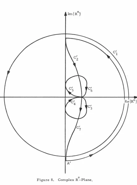
R -plane is shown in Fig. 8. Point A, which corresponds to 71. = -ir,

.), Segment Range of X. nd (x.) n ( x.) R' -(x.) of C s c2 O+i n, co >'fl;;:o:O

i

Jk

~+n

2 iJk2+Tlz s

( 21

}+k

2)

2

_

4

T1

2Jk~+T12

Jk2 +T12 +iNk 2T12 Jk 2 +T12 . s s s s c3 s +io , o:-:;; s:o:;;kd iJk 2 -s 2 d iJk2-s2 s (zsz -kz)z+ 4 s z J

kz-s

z'-hz~r!--iNkzr;Jkz -sz s d s . s s c4 s+iO, kd :o:;;g:o:;;k 8 Jsz-kz d i Jk

2 -s

2 s (Zsz-kz) 2- 4if,2Js2-k2

fk.~r--_

iNk2 s2Jk2 -s2 s -d s s s

J

s2 -k2 i Jk 2 -s 2 ( zs 2 -k 2 ) 2 +

4i s 2 J s 2 -k

2 J

k

2

-s

2 +

iNk 2 s 2 Jk 2

-~

cs s +iO, k 8 ;;::g;;::kd d s s d s s s c6 s+io, kd;;::g;;::o -i Jk

2 -s

2 iJk2-g2 (2S2-k2) 2 +

4~Jk2-~

Jk2-s2 -+ iNk2 s2.£2-s2 d s s d d s s c7 O+iT],0:2':T]> -co -iJ

k2+T12 d

i[k2;T1

2

s

( 2

T12+k2)2

_ 4

-56-Re