Generalized Wireless Network Coding Schemes for
Multi-Hop Two-Way Relay Channels
Gengkun Wang, Wei Xiang,
Senior Member, IEEE, and Jinhong Yuan,
Senior Member, IEEE
Abstract—Due to the overwhelming complexity of multi-hop transmission and inter-message interference, only a limited amount of research has been carried out in the implementation of wireless network coding (WNC) for generalized multi-hop two-way relay channels (MH-TRCs), let alone the generalization of multi-hop wireless network coding (MH-WNC) schemes. Our recent work showed that the MH-WNC scheme with fixed two transmission time intervals was unable to always outperform conventional Non-NC schemes in outage performance for the MH-TRC with an arbitrary number of nodes. In view of this fact, a generalized MH-WNC scheme with multiple transmission time intervals (TTIs) is designed for theL-nodeK-message MH-TRC in this paper. Closed-form expressions for the upper bound of the outage probability for two prominent relaying network coding strategies (i.e., analog network coding and compute-and-forward network coding) are derived. Moreover, by investigating the relationships between the outage probability and the numbers of nodes, messages and TTIs, we obtain an optimal MH-WNC scheme which can achieve the best outage probability and always outperform Non-NC in the MH-TRC with an arbitrary number of nodes.
Index Terms—Multi-hop wireless network coding, multi-hop two-way relay channels, outage probability, analog network coding, compute-and-forward network coding.
I. INTRODUCTION
M
ULTI-HOP networks, such as wireless sensor networks [1], wireless mesh networks [2], mobile ad hoc net-works [3], vehicular ad hoc netnet-works [4], have emerged as promising approaches to provide more convenient wireless communications due to their extended coverage, easy de-ployment and low costs. However, multi-hop wireless relay communications require an increase number of time slots to transmit data in a multi-hop manner [5] [6]. Information is conveyed through a series of intermediate relays in a conventional hop-by-hop and message-by-message manner, which limits network throughput, and thus the data rate of the system. The advent of network coding (NC) has offered a new opportunity to improve network throughput and reliability by exploiting interference in intermediate relays [7].Combined with network coding and self-information can-celation, wireless network coding (WNC) for two-way relay channels (TWRCs) has come to the forefront [8] [9]. There is a large body of work on the implementation and performance analyse (including outage probability, bit-error-rate and sum-rate) of WNC in the TWRC [10]–[12]. Subsequent work in
Gengkun Wang and Wei Xiang are with the Faculty of Health, Engineering and Sciences, University of Southern Queensland, Toowoomba, QLD 4350, AUSTRALIA (e-mail:{gengkun.wang, wei.xiang}@usq.edu.au)
Jinhong Yuan is with the School of Electrical Engineering and Telecommu-nications, University of New South Wales, Sydney, NSW 2052, AUSTRALIA (e-mail: [email protected]).
extending WNC to multi-hop two-way relay channels (MH-TRC) soon followed. Zhang et al. [8] described physical-layer network coding (PNC) for general uni-directional and bi-directional linear networks, which can achieve the upper-bound capacity of 0.5 frame/time slot in each direction for bi-directional transmissions between two end nodes [13]. However, there is no performance analyse presented in this paper. More recently, Youet al.applied analog network coding (ANC) to the MH-TRC in [14] [15], where the proposed AF-ANC-Central and AF-ANC-Even schemes can improve the network throughput compared to Non-NC schemes. However, there is no work on a generalized ANC transmission scheme for the MH-TRC with an arbitrary number of hops (referred to as all-scale MH-TRCs), and there is no published work on outage performance for such generalized MH-TRC networks, either.
Our previous work [16] [17] generalized the multi-hop wireless network coding (MH-WNC) scheme with fixed two transmission time intervals (TTIs) (referred to as2-TTI MH-WNC) for theL-nodeK-message MH-TRC. The2-TTI MH-WNC scheme was proven to markedly improve the spectral efficiency over conventional Non-NC schemes. However, it was also shown that the 2-TTI MH-WNC scheme is unable to outperform Non-NC for all-scale MH-TRCs. The multi-hop analog network coding (MH-ANC) scheme [16] can only outperform Non-NC in the MH-TRC with a small number of nodes, while the multi-hop compute-and-forward (MH-CPF) scheme [17] has better outage performance than Non-NC only for the MH-TRC with a large number of nodes.
The major contributions of this paper are multifold, which are summarized as follows:
• Proposal of a generalized transmission scheme of I-TTI MH-WNC for the L-nodeK-message MH-TRC; • Derivation of closed-form expressions for the upper
bound of the outage probability expressions of the MH-ANC and MH-CPF schemes;
• Evaluation of the relationships between the outage prob-ability and the numbers of nodes, messages and TTIs; and
• Identification of the optimal MH-WNC scheme which can achieve the best outage performance and outperform Non-NC for all-scale MH-TRCs.
The remainder of the paper is organized as follows. In Section II, the system model of the generalized L-node K -message MH-TRC and transmission schemes are presented. Outage performance of MH-ANC is discussed in Section IV. We then analyse the outage probability of MH-CPF in Section V. The optimal MH-WNC scheme is presented in Section VI. Finally, concluding remarks are drawn in Section VII.
The notation used herein is given in Table I.
TABLE I NOTATIONS.
Notation Definition
Pl Power per transmission for nodeNl
PS Single-access transmission power vector
PM Multiple-access transmission power vector
S Spectral efficiency
C Network throughput
yjl Received signal at nodeNlin time slotj
xjl Transmitted signal at nodeNlin time slotj
TIL,K Transmission pattern matrix forI-TTI MH-WNC in a
L-nodeK-message MH-TRC
Tvk Transmission pattern matrix for messagevk
Nvk Noise matrix for messagevk
˜
Nvk Noise power matrix for messagevk
Svk Signal matrix for messagevk
˜
Svk Signal power matrix for messagevk
Svk Single-access matrix for messagevk
˜
Svk Single-access power matrix for messagevk
PoutS,vk Single-access outage probability matrix for messagevk
Cvk Multiple-access matrix for messagevk
˜
Cvk Multiple-access power matrix for messagevk
PoutC,vk Multiple-access outage probability matrix for messagevk
II. SYSTEMMODEL
Consider an MH-TRC with L nodes {Nl}Ll=1, where user nodes N1 and NL exchange messages through intermediate relay nodes {Nl}L−l=21. The message sequences to be trans-mitted by N1 and NL are denoted by U = {uk}Kk=1 and
V={vk}Kk=1, and the modulated signal sequences are defined as Uˆ = {uˆk}Kk=1 and Vˆ = {vˆk}Kk=1. It is assumed that only immediately neighboring nodes are within the transmis-sion range in this network, and signals received from non-neighboring nodes are negligible due to signal attenuation.
In this paper, the overall system transmission power is assumed to be the same for both Non-NC and I-TTI MH-WNC schemes. Each node is assigned with transmission power
P for one message exchange, i.e., each node is allocated with transmission power2KP forK-message exchange. The greater the number of transmissions required at a node, the smaller the power per transmission will be. Denote by nl the total number of transmissions at node Nl, the power per transmission forNl is thus Pl= 2KP /nl.
The channel coefficient between nodes Nl and Nl+1 is denoted by {hl}L−l=11, which is considered quasi-static and reciprocal in bi-direction. For Rayleigh fading channels,hl∼ CN(0,2α2l) is modeled as a zero mean, independent, circu-larly symmetric complex Gaussian random variable with vari-anceα2l per dimension.{ωl}Ll=1 is the received noise at node
Nl, which is a zero mean, independent, circularly symmetric, complex Gaussian random variable with the variance of σ2.
γ0
l = |hl|2/σ2 is the signal-to-noise ratio (SNR) of hop l, which is exponentially distributed with parameter1/¯γ0l, with
¯
γ0l= 2α2l/σ
2 indicating the average SNR of the channel.
A. Non-Network Coding
In this paper, we consider the multi-hop communication system to be symmetrical in terms of user message exchange. That is, the two end users exchange their messages one by one at an equal rate, and the exchange sequence is {(u1, v1),(u2, v2), ...,(uK, vK)}.
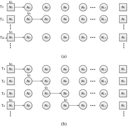
In conventional Non-NC schemes, intermediate terminals relay the signal from one hop to the next, as illustrated in Fig. 1(a). In non-regenerative systems, relays may amplify and forward the received signal from the previous node, whereas relays decode the signal and re-encode it prior to retransmission in regenerative systems. It takes L−1 time slots to forward one message from N1 to NL, and a total number of TNon-NC = 2K(L−1) time slots are required to complete the message exchange.
Spectral efficiency for the MH-TRC is defined as the number of messages transmitted in a single time unit. Thus, the spectral efficiency of this conventional Non-NC scheme is
SNon-NC= 1/L−1.
It should be noted that for the symmetrical message ex-change pattern {(u1, v1),(u2, v2), ...,(uK, vK)}, the above conventional Non-NC scheme is the only scheme to avoid interference. However, if the symmetrical message ex-change pattern is not required, e.g., the exex-change sequence is {(u1, u2, ..., uK),(v1, v2, ..., vK)}, another asymmetrical Non-NC scheme can be applied, as shown in Fig. 1(b). Under this scheme, each node forwards the received signal to the next neighboring node every three time slots, and the transmissions do not overlap due to the two-hop intervals between them, as illustrated in Fig. 1(b) at time slot T4. The total number of time slots required for this asymmetrical Non-NC scheme is
2(L−1)+6(K−1), and the spectral efficiency isSAsy-Non-NC=
K/((L−1) + 3(K−1)). When the number of messagesK
is far larger than the number of nodes L, an upper limit can be obtained as SˆAsy-Non-NC= lim
K>>L K
(a)
[image:3.612.64.287.58.276.2](b)
Fig. 1. (a) Conventional Non-NC scheme. Nodes N1 and NL take turns
to transmit their messages until the end of the exchange process. Node NL starts transmitting its message vk after receiving the corresponding
messageukfrom its counterpartN1, and so forth. The transmission pattern is {(u1, v1),(u2, v2), ...,(uK, vK)}; (b) Asymmetrical Non-NC scheme.
User nodeN1transmits a new message every three time slots. For example, when nodeN4 transmits messageu1 to N5 in the fourth time slot, node
N1sendsu2 toN2 at the same time. NodeNLstarts sending its messages
after receiving all the K messages from node N1, and follows the same transmission pattern as node N1. The transmission pattern is{(u1, u2, ...,
uK),(v1, v2, ..., vK)}.
one user node does not start sending its messages until it re-ceives all the messages from its counterpart, which causes long delays in message exchange for this user node. Moreover, the resultant unequal message exchange leads to traffic imbalance and user unfairness issues between the two user nodes, in comparison with the symmetrical message exchange pattern. Furthermore, the asymmetrical exchange pattern is different from the symmetrical one, which is widely considered in the literature, e.g., the WNC scheme for the TWRC [8] [9] and the MH-WNC scheme for the MH-TRC [13] [14]. Therefore, the asymmetrical Non-NC scheme is not considered in this paper, and the Non-NC scheme we refer to in the following sections is the conventional Non-NC scheme illustrated by Fig. 1(a).
B. Generalized Wireless Network Coding Scheme
We now introduce WNC into theL-nodeK-message MH-TRC. Without loss of generality, we only consider that the number of nodes L is odd in this paper, while the case of even L can be easily extrapolated from the same procedure presented in this section.
Instead of sending their messages every two time slots as in the 2-TTI MH-WNC scheme, the two user nodes send one message every I > 2 time slots simultaneously, and the messages sent by N1 and NL in time slot j ∈ {1, I+
1, ..., IK−1}areu(j−1)/I+1 and v(j−1)/I+1, respectively. A total number of IK−1 time slots is required for the two user nodes to complete sending their message sequences.
Once the relay receives the messages from both neighboring nodes, it network-codes the received signal, and broadcasts the network-coded message to the neighboring nodes in the next transmission time slot. The received signal of the multiple-access phase at relay nodeNl in time slotj is given by
ylj = pPl−1hl−1xjl−1+
p
Pl+1hlxjl+1+wjl, (1)
where xjl is the transmitted signal by relay node Nl in time slot j, and wjl denotes the received noise at node Nl in time slot j. For non-regenerative relaying strategies, the transmitted signalxjl is simply a scaled version of the received signal from the previous time slot ylj−1. For regenerative relaying strategies, the transmitted signal xjl is a network-coded codeword denetwork-coded fromylj−1(an XORed message with “standard” PNC, or a linear combination with CPF).
After time slot L−1, the two user nodes N1 and NL will receive the signal containing the messages from the counterpart every I time slots. Knowing its own messages, the user nodes can extract the required messages. For the non-generative MH-TRC, the user nodes cancel their own signals and decode required messages. On the other hand, the user nodes decode the linear combination of outgoing and incoming messages, and solve the linear equations for the required messages in the regenerative MH-TRC.
Let R, T and denote the receiving, sending and silent modes of the nodes, respectively. Denote bySjl the operation mode for node Nl in time slot j. The transmission modes for each node in different time slots with MH-WNC can be summarized as
• For user nodesN1 andNL:
Sj1=S j
L=T,j∈ {1, I+ 1,2I+ 1, ...,(K−1)I+ 1}. Sj1=S
j
L=R,j ∈ {L−1, L−1 +I, L−1 + 2I, ..., L−
1 +I(K−1)}. Sj1=S
j
L= , other. • For relay nodes{Nl}L−l=21:
Sjl = T, j ∈ {L−l+ 1, L−l+I+ 1, L−l+ 2I+
1, ..., L−l+ (K−1)I+ 1} ∪ {l+ 1, l+I+ 1, l+ 2I+ 1, ..., l+ (K−1)I+ 1}.
Sjl =R, if S j
l−1=T∪S j l+1=T.
Sjl = , other.
Let −1 represent the single-access mode, 1 represent the transmission mode, 0 represent the silent mode, and −2
represent the multiple-access mode. The transmission pattern can be represented by aT (the number of time slots) byL(the number of nodes) transmission matrix TI
L,K. For example, the transmission matrix of 2-TTI MH-WNC for the 5-node
2-message MH-TRC can be expressed as
T25,2=
1 −1 0 −1 1
0 1 −2 1 0
1 −2 1 −2 1
−1 1 −2 1 −1
0 −1 1 −1 0
−1 1 0 1 −1
, (2)
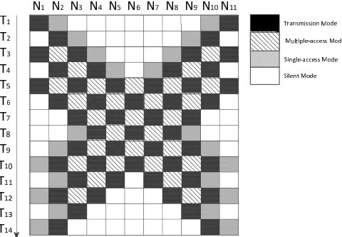
slotj. For example, the first row [1,−1,0, ,−1,1]represents that N1is transmitting a message toN2,N5is transmitting a message toN4, andN3is in the silent mode. In this paper, we devise a grid chart to display the transmission pattern via the matrix, e.g., the grid chart of2-TTI MH-WNC for the11-node
[image:4.612.56.296.150.316.2]3-message MH-TRC is illustrated in Fig. 2.
Fig. 2. Grid chart of2-TTI MH-WNC for the11-node3-message MH-TRC. The horizontal grids represent the Lnodes, and the vertical grids represent theT time slots. The colour of each grid indicates the operation mode of the corresponding node in a specific time slot.
With I-TTI MH-WNC, the total number of time slots for exchanging the two message sequences is TMH-WNC =
L −1 +I(K −1). The spectral efficiency is SMH-WNC =
2K/(L−1 +I(K−1)). When the number of messages is far larger than the number of nodes, an upper limit of SMH-WNC can be obtained as SˆMH-WNC = lim
K>>L−1−I 2K
L−1+I(K−1) =
2/I. In comparison with Non-NC, the generalized MH-WNC scheme markedly improves the spectral efficiency.
III. OUTAGEPERFORMANCE OFMULTI-HOPANALOG
NETWORKCODING
In this section, we will analyse the performance of MH-ANC for the non-regenerative MH-TRC, including the average received SNR and outage probability.
There is a large body of literature on the performance analyse of the traditional amplify-and-forward (AF) scheme in multi-hop relay networks, which is related to the work presented in this section. Hasna et al. [20] derived the an-alytical expressions of the harmonic mean and cumulative density function of the average received SNR for two-hop relay networks, which can be applied to outage performance and average bit-error-rate (BER) analyse. Then, they gener-alized the outage probability of the multi-hop relay network over Nakagami fading channels in [21]. In [11], the authors analysed the performance of ANC in a single relay TWRC. Closed-form expressions of the average received SNR, outage probability, sum-bit-error-rate and maximum sum-rate for the traditional three time slot network coding, and ANC schemes
were derived. In this paper, this previous work on the non-regenerative MH-TRC will be used as a benchmark in the outage performance analyse.
The AF relaying strategy is applied at each relay in MH-ANC, and the transmitted signal of relay nodeNl in time slot
j is a scaled version of the received signal in the previous time slotxjl =Glyj−l 1, whereGl represents the gain at relay nodesNl, which is set to
G1l = s
1
Pl−1|hl−1|2+σ2
, Nl−1
a
→Nl, (3)
G2l = s
1
Pl|hl|2+σ2
, Nl
a
←Nl+1, (4)
G3l = s
1
Pl−1|hl−1|2+Pl+1|hl|2+σ2
, Nl−1 a →Nl
a0
←Nl+1(5).
whereNl−1 a
→Nl denotes that Nl−1 transmits message ato
Nl. After time slotL−1, the two user nodes will receive the signal containing the messages from the counterpart user node everyI time slots. Knowing their own messages, user nodes can cancel these signals in the analog field and decode the required messages.
A. Received SNR
For the MH-ANC scheme, the message is amplified and forwarded bi-directionally at the relay nodes throughout the exchange process. Hence, the received signal atN1consists of the outgoing messages, incoming messages, and the received noise at intermediate relays. For the L-node MH-TRC with aI-TTI MH-ANC scheme, the received signal at N1 can be expressed as (6), (7) and (8), where ψi,lj ,ϕji,l andφjl are the polynomials ofPl,Glandhlfor termuˆi,ˆviandωljat time slot
j, respectively. In this paper, it is assumed that the two user nodes have the knowledge of the channel state information (CSI) of the channels, via pilot transmission during which the CSI can be estimated and passed to the user nodes. Note that N1 has the knowledge of its own transmitted messages {u1, u2, ..., uK}, it can cancel the terms of uˆi and extract ˆv1 at time slot L−1, as shown in (6). At time slotL−1 +I,
N1 can extractˆv2 with the knowledge of its own transmitted messages and the message ˆv1 extracted at time slot L−1, as shown in (7). The operation continues to decode all the incoming messages everyI time slots.
Hence, the resulting signal of message vk after canceling the outgoing and previously extracted messages can be derived from (8) as
y∗MH-ANC,vk =
X
l∈{1,L},j∈{1,TMH-ANC,vk}
ϕjk,lˆvk+φjlω j l
. (9)
The received SNR of messagevk can be obtained as
γMH-ANC,vk =
P
l∈{1,L},j∈{1,TMH-ANC,vk} |ϕjk,l|2
P
l∈{1,L},j∈{1,TMH-ANC,vk}
|φjl|2σ2. (10)
yMH-ANC,v1 = bL−1
I c
X
i=1
X
l∈{1,L},j∈{1,L−1}
ψji,luˆi+
X
l∈{1,L},j∈{1,L−1}
ϕj1,lˆv1+
X
l∈{1,L},j∈{1,L−1}
φjlωlj, (6)
yMH-ANC,v2 = bL−1+I
I c
X
i=1
X
l∈{1,L},j∈{1,L−1+I}
ψi,lj uˆi+
X
l∈{1,L},j∈{1,L−1+I}
ϕj1,lvˆ1+
X
l∈{1,L},j∈{1,L−1+I}
ϕj2,lvˆ2
+ X
l∈{1,L},j∈{1,L−1+I}
φjlωjl, (7)
...
yMH-ANC,vk =
bTMH-ANCI ,vkc
X
i=1
X
l∈{1,L},j∈{1,TMH-ANC,vk}
ψji,luˆi+ k−1
X
i=1
X
l∈{1,L},j∈{1,TMH-ANC,vk}
ϕji,lˆvi
+ X
l∈{1,L},j∈{1,TMH-ANC,vk}
ϕjk,lvˆk+
X
l∈{1,L},j∈{1,TMH-ANC,vk}
φjlωlj, (8)
———————————————————————————————————————————————————–
binary phase-shift keying (BPSK) modulation is used at all the nodes.
Two recursive approaches were proposed in [16] to derive the analytical polynomials ϕjl and φjl for the 2-TTI MH-ANC. However, it is difficult to devise an universal recur-sive approach for the generalized I-TTI MH-ANC scheme, because the transmission patterns are different for the MH-ANC schemes with different TTIs. Therefore, by utilizing the transmission pattern matrix of each message, we design a numerical algorithm to compute ϕjl andφjl, thus the received SNR for each message.
For the purpose of theoretical analysis and following other work in the literature [22] [23], we assume that all the channels have the same amplitude, i.e., |hl|2 = |h|2. It is noted that this assumption is only made for analytical convenience. i.e., the derivation of outage performance and the comparison with the conventional Non-NC schemes. The implementation of the protocol in practical communications networks will not be constrained by this assumption due to the availability of some practical mechanism such as pilot transmission to acquire the CSI of the channels before message exchange.
Denote by{Wl}Ll=1the weight as the power of amplification factor at each node, three different weights corresponding the amplification factors given by (3), (4) and (5) at node Nlcan be obtained as
Wl1= Pl|h|
2
Pl−1|h|2+σ2
, Nl−1
a
→Nl, (11)
Wl2= Pl|h|
2
Pl+1|h|2+σ2
, Nl
a
←Nl+1, (12)
Wl3= Pl|h|
2
(Pl−1+Pl+1)|h|2+σ2
, Nl−1 a →Nl
a0
←Nl+1.(13)
Since only some transmission events affect the noise propa-gation, the transmission matrix for each message can be further converted into a characteristic matrix that only contains the effective transmission events. By applying different weights into these transmission events, the noise power matrix for
messagevk can be computed as
˜ Nvk =
3
X
i=1
Nivk◦Wi, (14)
whereNi
vkis the noise matrix containing only the transmission event with weight Wi
l, and A◦B = [aij]m×n◦[bj]n×1 =
[aij∗bj]m×n.
The propagation of the noise power is simply the traversal of the weights at each non-zero node in the noise power matrix. The following post-order traversal approach is proposed to obtain the noise power.
Algorithm: Post-order traversal algorithm for the
noise power matrix Nvk
Input:Noise power matrix Nvk. Output:Noise power Nvk.
1.Nn=ZEROS(Ti×L)
2.fori=1 toTi do
3. forj=1 toLdo
4. ifCvi(i, j) = 0then
5. Nn(i, j)←0
6. end if
7. ifCvi(i, j)6= 0 then
8. Nn(i, j)←(Nn(i+ 1, j−1)
+Nn(i+ 1, j+ 1))×Cvi(i, j)
9. end if
10. end for
11.end for
12.returnNvk←SU M(Nn) + 1
the noise power matrix as
NMH-ANC,vk=Trv
˜ Nvk
σ2, (15)
where Trv(·)stands for the post-order traversal algorithm. Similarly, the signal power matrix can be obtained as
˜ Svk=
4
X
i=1
Sivk◦Wi
, (16)
where Sivk is the signal matrix containing only the transmis-sion event with weightWi
l, andW
4={W4
l =Pl|h|2}Ll=1. The signal power is simply the product of all non-zero elements in the signal power matrix, given by
SMH-ANC,vk =Prodnz
˜ Svk
, (17)
where Prodnz(·)indicates the product of all non-zero elements of the matrix.
Then, the received SNR of messagevkcan be calculated by dividing the signal power in (17) by the noise power in (15) as
γMH-ANC,vk = SMH-ANC,vk NMH-ANC,vk
=
Prodnz
˜ Svk
TrvN˜vk
σ2
. (18)
B. Upper Bound of the Received SNR
In high SNR regions, the three weights given by (11), (12) and (13) can be upper-bounded as
ˆ
Wl1= Pl|h|
2
Pl−1|h|2+σ2
=
2KP nl γ
0
2KP nl−1γ
0+ 1
γ0→∞
= nl−1
nl
,(19)
ˆ
Wl2= nl+1
nl
, (20)
ˆ
Wl3=
nl−1nl+1
nl(nl−1+nl+1)
, (21)
where nl is the total number of transmissions of node Nl, which is constant only determined by L, K, I.
Therefore, it can be deduced that, in high SNR regions, the noise power given by (15) is a scaled version ofσ2, i.e.,fkNσ2, and the signal power given by (17) is also a scaled version of
W4
l =Pl|h|2, i.e., fkSPl|h|2=
fkS2KP|h|2
nl , the received SNR of vk given by (18) can be simplified as
ˆ
γMH-ANC,vk =
fS k2KP|h|2
nl
fN k σ2
=fkP γ0, (22)
whereγ0= |h|σ22 andfk= fS
k2K fN
knl .
The upper bound of the average received SNR for the L -node K-message MH-TRC can be given by
ˆ
γMH-ANC = 1
K
K
X
k=1
ˆ
γMH-ANC,vk = 1
K
K
X
k=1
P fkγ0 =FKP γ0,(23)
whereFK= K1 K
P
k=1
fk.
C. Outage Probability
The maximum mutual information forI-TTI MH-ANC can be shown as
IMH-ANC = CMH-ANClog(1 +γMH-ANC). (24)
Given a target rate R, the upper-bound outage probability in high SNR regions can be derived as
ˆ
poutMH-ANC(R) = Pr[CMH-ANClog (1 +FKP γ0)< R]
=Fγ0
2CMH-ANC1 R−1 FKP
!
= 1−exp
−2 1
CMH-ANCR−1
FKP¯γ0
| {z }
A , (25)
whereFγ0(x)is the cumulative density function (CDF) ofγ0. The outage probability given in (25) can be computed analytically, because that bothCMH-ANC andFK are constants and can be readily obtained by the algorithms presented in this section. More specifically, the received SNR derivation example for message v1 in the 5-node 2-message MH-TRC with2-TTI MH-ANC is presented in Appendix A to explain the derivation.
IV. OUTAGEPERFORMANCE OFMULTI-HOP
COMPUTE-AND-FORWARDNETWORKCODING
Compute-and-forward network coding strategy was pro-posed recently to realize reliable PNC [24], where the relays compute and forward linear combinations of user messages to destinations. It is noted that for BPSK, when the two integer coefficients are set to1in a two-user multiple-access channel, the linear combination is equivalent to the modular-2 addition in “standard” PNC [8], which is also implied in [25, Remark 4] and [26, Section II-B].
In MH-CPF, relay nodes compute linear combinations of messages from neighboring nodes and broadcast to them in next transmitting time slots. The received signal given by (1) can be rewritten as
yjl =Dl
h
xjl−1 xjl+1i
T
+wjl, (26)
where Dl = [
p
Pl−1hl−1
p
Pl+1hl], x j
l−1 and x j
l+1 are the transmitted signals from neighboring relay nodes Nl−1 and
Nl+1, which are the decoded linear combinations at the relay nodes in the previous time slot.
After receiving the interference signal, the relay node selects a complex integer coefficient vector ajl ∈ {Z+Zi}2 and decodes the following linear combination
xlj=ajlhxl−j−11 xj−l+11i
T
. (27)
and the complex integer coefficient vector ajl, the user nodes are able to solve the linear combination for their required messages.
In this paper, all the channels are assumed to be quasi-static, implying that the instantaneous channel state information of
hl remains unchanged during the entire exchange process. Therefore, the maximized computation rate RCOMP,l(hl,a
j l) for decoding the linear combinationxjl at relayNl disregards the time slot j, and remains unchanged during the entire exchange process. Thus, the computation rate at relay Nlcan be given by [25]
RCOMP,l(Dl,ˆal) = log+ ||ˆal||2−
|ˆalD†l|2
n0+||Dl||2
!−1
,(28)
where log+(x) , max (log(x),0) and ˆal = [~al, ~al]. ~al and l~a are two complex integer coefficients corresponding to
the two messages xj−l−11 and xlj−+11 in linear combination xjl, respectively. According to Theorem 1 in [27] and Proposition 1 in [28], the above maximization problem amounts to the following shortest vector problem (SVP),
ˆ
al= argmin
al6=0||alL||, (29)
where L is the Cholesky decomposition matrix of I −
D†lDl
n0+||Dl||2, andIis anL×Lidentity matrix.
For the above special two-dimensional case in Rayleigh fad-ing channels, the complex lattice reduction algorithm proposed in [29] can be applied to solve the above SVP and obtain the maximized computation rate efficiently.
Each message follows a different transmission path, and failing to decode one message will affect the decoding of the following messages. The outage probabilities of later messages are poorer than those of early messages.
Given a target rate R, the average outage probability per message is defined as
pout(R)=1
K
K
X
k=1
poutvk(R), (30) wherepout
vk(R)is the outage probability of messagevk, which is identical to the outage probability of messageuk due to the symmetrical property of the two-way transmission. The outage event of messagevkoccurs when any of the transmissions that affect the transmission of message vk are in outage.
In order to determine the outage probability for each mes-sage, we first define fS,lj and fM,lj as the single-access and multiple-access transmission events at nodeNlin time slotj,
fS,lj ,
Nl−1 a
−−→Nl ∪Nl a
←−−Nl+1 ,
fM,lj ,
Nl−1 a −−→Nl
a0
←−−Nl+1 , ∀l∈ {1,2, ..., L},∀j ∈ {1,2,3, ...},
and Fvk as the set of all the transmission events that affect the transmission of messagevk,
Fvk,
n
{fS,lj , fM,lj }l∈{j∈{11,,22,...,L},...,Tk}o, ∀k∈ {1,2, ..., K},
Thus, the outage event of message vk occurs when any
single access transmission eventfS,lj or multiple-access trans-mission evensfM,lj in set Fvk is in outage, given by
poutv
k(R) = 1−
Y
fS,lj ∈Fvk
1−pout
fS,lj (RMH-CPF)
| {z }
Bk
Y
fM,lj ∈Fvk
1−pout
fM,lj (RMH-CPF)
| {z }
Ck
, (31)
whereRMH-CPF is the message target rate for each transmis-sion, given byRMH-CPF=R/CMH-CPF.
A. Single-Access Transmission Event
The single transmission event matrix Svk can be extracted from the transmission pattern matrix of message vk, by setting to 1 the corresponding elements (whose left or right neighboring element in the transmission matrix Tvk is −1). For example, the single access transmission matrix of message
v1 for the 5-node 2-message MH-TRC with2-TTI MH-CPF scheme can be obtained as
Sv1 =
1 0 0 0 1
0 0 0 0 0
0 0 1 0 0
0 1 0 0 0
. (32)
It is assumed that all the channel coefficients are iden-tical. Therefore, for the single access transmission, the outage probability is only determined by the transmission power at each transmission. The transmission power vec-tor of the L-node MH-TRC can be written as PS =
[P1 P2 P3· · ·Pl· · · PL], wherePlis the power per trans-mission of node Nl.
The single access transmission power matrix (each element denotes the transmission power of the corresponding transmis-sion event) can be obtained as
˜
Svk =Svk◦PTS. (33)
Given a target rateR, the single access transmission outage probability matrix of messagevk (the elements are the outage probability of each single access transmission) can then be written as
PoutS,vk =J L
Tvk −exp −
(2CMH-CPFR −1)
¯
γ .∗
˜
Svk
!
, (34)
whereJL
Tvk is aTvk byLmatrix of ones, and (.∗) represents element-wise multiplication operation.
The element in PoutS,vk is the outage probability of all the single access transmission events that affect the transmission of messagevk. Therefore, termBk in (31) can be obtained as
Bk =Prod
JTvk,L−PoutS,vk
where Prod(·)represents the product of all the elements in the matrix.
B. Multiple-Access Transmission Event
It is assumed that all the channels have the same am-plitude, i.e., |hl|2 = |h|2. Therefore, the computation rate is determined only by the transmission powers of the neighboring nodes and the integer coefficient vector aˆl, as can be seen from (28). Hence, the power vector for the multiple-access transmission can be written as PM =
[PM,1 PM,2 PM,3· · ·PM,l· · ·PM,L], where each element
PM,l = (Pl−1, P1) contains the transmission powers of the two neighboring nodes of Nl, andPM,1=PM,L= (0,0).
The CPF matrixCvkcan be extracted from the transmission matrix of message vk, by setting the corresponding elements whose value in the transmission matrix Tvk is −2 to1. For example, the CPF matrix of message v1 for the 5-node 2 -message MH-TRC with the 2-TTI MH-CPF scheme can be obtained as
Cv1 =
0 0 0 0 0
0 0 1 0 0
0 0 0 0 0
0 0 0 0 0
. (36)
Multiplying the CPF matrixCvk by the power vectorPM, the CPF power matrix can be obtained as
˜
Cvk=Cvk◦P T
M. (37)
For a given target rate R, the CPF outage probability matrix whose elements are the outage probability of each CPF process, can then be given by
PoutM,vk=CPF
˜
Cvk
, (38)
where CPF(·) represents the algorithm for calculating the outage probability of each non-zero element. Due to page limitation, we are unable to include this algorithm here, while interested readers can refer to our previous work in [17].
The element in PoutM,vk is the outage probability for all the multiple-access transmission events that affect the transmis-sion of message vk. Therefore, term C in (31) can then be obtained as
Ck =Prod
JTvk,L−PoutM,vk
. (39)
Substituting (31) to (30), the outage probability for I-TTI MH-CPF can be obtained as
poutMH-CPF(R)
= 1 K
K
X
k=1
(1− Bk· Ck)
= 1− 1 K
K
X
k=1
"
ProdJTLvk−PoutS,vk
·ProdJTLvk −PoutM,vk
#
.(40)
It should be noted that, the two outage matrices PoutS,vk and PoutS,vkcan be readily obtained through the proposed algorithms. Moreover, the two matrices are only determined by L, K, I.
Therefore, the outage probability of theI-TTI MH-CPF for the
L-nodeK-message MH-TRC given by (40) can be computed analytically.
V. NUMERICALRESULTS
In this section, we will investigate the relationships between the outage probability and the numbers of nodes, messages, and TTIs ofI-TTI MH-WNC, so as to determine the optimal MH-WNC scheme for all-scale MH-TRCs. The transmission power per message P is normalized to 1 in the following numerical results.
The spectral efficiency of I-TTI MH-WNC is determined by the number of nodes (L), the number of messages (K), and the number of TTIs (I). Denote by fsp(L, K, I)the spectral efficiency function ofI-TTI MH-WNC, we have
• fsp(L, K, I1)< fsp(L, K, I2), ∀I1> I2, (41) • fsp(L, K1, I)> fsp(L, K2, I), ∀K1> K2, (42)
fsp(L, K, I)≈
2
I, ∀KL−1−I,(43)
• fsp(L1, K, I)< fsp(L2, K, I), ∀L1> L2. (44)
A. Multi-Hop Analog Network Coding
[image:8.612.294.565.243.459.2](a) (b)
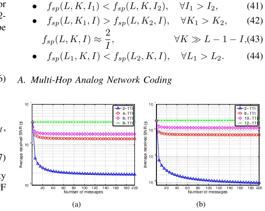
Fig. 3. Average received SNR versus the number of messages for the MH-TRCs of different scales. (a)9-node MH-TRC; and (b)13-node MH-TRC.
Fig. 3 plots the upper bound of the average received SNR (as given by (23)) for I-TTI MH-ANC versus the number of messages, where the average received SNR is measured by γ0 (the average SNR per hop). As can be seen from the figures, the average received SNR decreases with the number of messages whenI < L−1, and remains unchanged regardless of the number of messages when I = L−1. Moreover, the average received SNR becomes steady when the number of messages is large. The figure also demonstrates that the average received SNR of the MH-ANC scheme with larger TTIs is larger than the MH-ANC scheme with a smaller number of TTIs.
(a) (b)
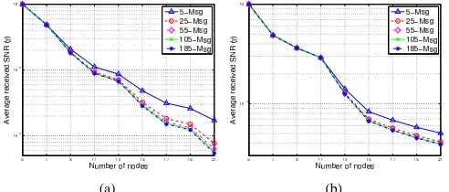
Fig. 4. Average received SNR versus the number of nodes for the MH-ANC scheme with various numbers of TTIs. (a)6-TTI MH-ANC; and (b)10-TTI MH-ANC.
Denote byfs(L, K, I)the average received SNR of theL -node K-message MH-TRC withI-TTI MH-ANC, we have
• fs(L, K, I1)> fs(L, K, I2),∀I1, I2< L−1, I1> I2,(45)
fs(L, K, I1)≡fs(L, K, I2), ∀I1, I2>L−1, (46) • fs(L, K1, I)< fs(L, K2, I),∀K1> K2, , (47)
fs(L, K1, I)≡fs(L, K2, I), ∀K1, K2L−1−I,(48) • fs(L1, K, I)< fs(L2, K, I),∀L1> L2. (49)
It can be inferred from (41), (42), (45) and (47) that the monotonic characteristics of the spectral efficiency with K, I
are actually opposite to that of the average SNR. Therefore, the numerator and denominator of term A in (25) have the same monotonous characteristics. It is difficult to determine the monotonic characteristic of the outage probability with
K, I only by Equation (25) intuitively. Lemma 1:Denote byfo
MH-ANC(L, K, I)the outage probabil-ity of theL-nodeK-message MH-TRC withI-TTI MH-ANC, we have
fMH-ANCo (L, K, I1)< fMH-ANCo (L, K, I2), ∀I1> I2, I1, I2>L−1,
Proof: The outage probability of theL-nodeK-message MH-TRC with I-TTI MH-ANC can be written as
fMH-ANCo (L, K, I) = 1−exp −2 R fsp(L,K,I)−1
fs(L, K, I)
!
, (50)
according to (25). For ∀I1 > I2, I1, I2 >L−1, substituting (41) and (46) into (50), Lemma 1 can be proved due to the monotonic property of the exponential function.
In this paper, we aim to determine the optimal MH-ANC scheme, amounting to identifying the number of TTIs for the optimal scheme. The number of TTIs is from I ∈ {2,4,6, ...,+∞}, and it is computationally intractable to enu-merate the list to determine the optimal TTI. However,Lemma 1 suggests that the outage probability of I-TTI MH-ANC increases with the number of time intervals when I > L−1
for the L-node K-message MH-TRC, meaning that the I -TTI MH-ANC scheme with I 6 L−1 can achieve better outage performance than those withI > L−1. Therefore, the following remark can be intuitively derived from Lemma 1.
Remark 1: The number of TTIs for the optimal MH-ANC scheme lies within {2,4, ..., L−1}.
It can be seen that Remark 1 significantly reduces the computational complexity of searching the number of TTIs for the optimal MH-ANC scheme. In the following section, we will present the outage probabilities of the I-TTI MH-ANC schemes withI6L−1with the aim of identifying the optimal MH-ANC scheme.
B. Optimal Multi-Hop Analog Network Coding
[image:9.612.313.559.161.274.2](a) (b)
Fig. 5. Outage probability versus the number of messages for the MH-TRCs of different scales. (a)5-node MH-TRC. The outage probability for2-TTI MH-ANC decreases with the number of messages, and the outage probability for4-TTI MH-ANC remains constant as the outage of early messages does not affect that of later messages; and (b)9-node MH-TRC. The outage probability of the 2-TTI MH-ANC scheme drops with the increase in the number of messages until a certain value, i.e., K = 4, and then rebounds after this value.
Fig. 5 plots the upper bound of the outage probability versus the number of messages. The average SNR per hop is set to
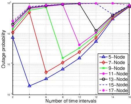
40 dB. It can be found that the outage probability converges to a constant value when the number of messages becomes large. Moreover, 2-TTI MH-ANC has a significantly better outage performance than4-TTI MH-ANC for the5-node MH-TRC. Therefore, the optimal MH-ANC scheme for the5-node MH-TRC is2-TTI MH-ANC. Similarly, the optimal MH-ANC scheme for the9-node MH-TRC is4-TTI MH-ANC.
As can be seen from Fig. 5, the outage probability of theI -TTI MH-ANC scheme reaches a stable value when the number of messages is far larger than the number of nodes. Therefore, we plot the upper bound of the outage probability versus the number of TTIs for the MH-TRCs of different scales with
K= 400in Fig. 6. The average SNR per hop is set to30dB.
As can be observed from Fig. 6, all the outage probability curves follow almost the same trend, in which the outage probability decreases with the number of TTIs when it is below a certain value, and reaches a valley point, then starts increasing after this valley point. Fig. 6 clearly shows the optimal MH-ANC scheme with the best outage performance for all-scale MH-TRCs. The number of TTIs for the optimal MH-ANC scheme is summarized in Table II.
Fig. 6. Outage probability versus the number of TTIs for the MH-TRCs of different scales withK= 400.
TABLE II
OPTIMALMH-ANCSCHEMES FOR THEMH-TRCS OF DIFFERENT SCALES.
Number of nodes (L) Number of TTIs (I)
5 2
7 4
9 4
11 4
13 6
15 6
17 8
19 6
21 10
23 8
25 8
27 10
29 10
31 10
Fig. 7. Outage probability for the optimal MH-ANC scheme versus the number of nodes.
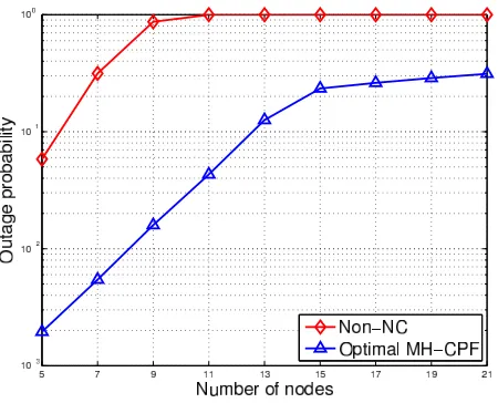
As demonstrated in [16], the outage performance gain of the 2-TTI MH-ANC scheme relative to the Non-NC scheme diminishes when the number of nodes becomes large. How-ever, as can be seen from Fig. 7, the outage probability of the optimal MH-ANC scheme is significantly better than that of the Non-NC scheme, and the gain increases with the number of nodes.
C. Compute-and-Forward Network Coding
In this section, the outage probability of the MH-CPF scheme is derived to determine the relationships with the numbers of nodes, messages, and TTIs, so as to determine the optimal MH-CPF scheme for all-scale MH-TRCs..
Lemma 2: Denoting by fo
MH-CPF(L, K, I)the outage prob-ability of the L-nodeK-message MH-TRC with I-TTI MH-ANC, we have
fMH-CPFo (L, K1, I) =fMH-CPFo (L, K2, I), ∀K1, K2, I >L−1.
fMH-CPFo (L, K, I1)< fMH-CPFo (L, K, I2), ∀I1> I2, I1, I2>L−1.
Proof: As inferred from the transmission scheme for I -TTI MH-CPF, whenI>L−1, the second outgoing message is transmitted after the first incoming message reaches the user node. There is no inter-message interference, meaning that the transmission of each message does not interfere with each other. Therefore, the outage probability for each message is equivalent to each other, which leads to the first statement in Lemma 2.
Moreover, the number of transmission events that affect the transmission of each message remains unchanged with the increase of the number of TTIs when I > L−1. Denote by Fvk(L, K, I)the set of transmission event that affect the transmission of messagevk, we can obtain
Fvk(L, K, I)≡ Fvk(L, K, L−1),∀I>L−1. (51)
where≡stands for identically equal.
On the other hand, the spectral efficiency decreases with the number of nodes, causing the drop of the message rate. As can be seen from (31), when I > L−1, the numbers of components in terms Bk and Ck remain unchanged with the number of TTIs, while, the outage probabilities for each component in terms Bk and Ck decrease with the increased number of TTIs due to the decrease of the message rate for each transmission. Therefore, termsBkandCkin (31) decrease with the increased number of TTIs, which proves the second statement inLemma 2.
Similar to the situation in MH-ANC, the following remark can be intuitively derived from Lemma 2 to simplify the identification of the optimal number of TTIs for the MH-CPF scheme.
Remark 2: The number of TTIs for the optimal MH-CPF scheme lies within{2,4, ..., L−1}.
In the following section, only the outage probabilities of the
D. Optimal Compute-and-Forward Network Coding
[image:11.612.323.549.58.238.2](a) (b)
Fig. 8. Outage probability versus the number of messages for the MH-TRCs of different scales. (a) 9-node MH-TRC. The outage probability for2-TTI MH-CPF sees a valley point when the number of messages is approximately6, whilst the other curves withI < L−1increase with the number of messages. The outage probability of8-TTI MH-CPF remains constant regardless of the number of messages; and (b)15-node MH-TRC.
Fig. 8 shows the outage probability versus the number of messages. The average SNR per hop is set to 20 dB. It can be clearly seen that the outage probability for I-TTI MH-CPF with I < L−1 generally increases with the number of messages. Moreover, whenI=L−1, the outage probability remains unchanged despite the increased number of messages, as indicated by Lemma 2. Fig. 8(a) shows that the outage probability of the(L−1)-TTI MH-CPF scheme is larger than the MH-CPF scheme with I < L−1 when the number of messages is small. However, the outage probability of the MH-CPF scheme with I < L−1 increases quickly with the increase in the number of messages. As a result, the (L−1) -TTI MH-CPF scheme has better outage performance than the other schemes when the number of messages is large.
On the other hand, as can be observed from Fig. 8(b), the
2-TTI MH-CPF scheme is always superior to the14-TTI MH-CPF scheme in the 15-node MH-TRC, when the number of messages is smaller than400. However, the outage probability of 2-TTI MH-CPF keeps increasing when the number of messages is larger than 400. Therefore, it can be interpreted that the outage probability of2-TTI MH-CPF will exceed that of 14-TTI MH-CPF when the number of message reaches a certain value (the number is 620 as our experiment results suggest).
Based upon the above discussions, it can be concluded that when the number of messages is relatively small,2-TTI MH-CPF is the optimal MH-MH-CPF scheme for all-scale MH-TRCs. However, when the number of messages becomes relatively large, the optimal MH-CPF scheme is (L−1)-TTI MH-CPF. As an example, we plot the outage probability versus the number of TTIs in Fig. 9 with the number of messages400.
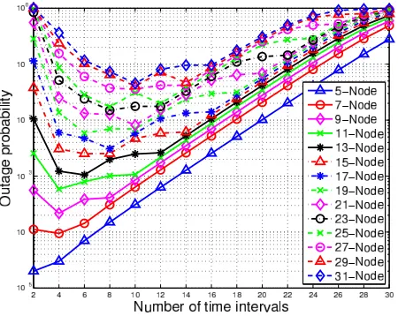
As can be seen from Fig. 9, all the outage probability curves have a valley point. This point moves rightwards with the increase in the number of nodes. However, the figure also suggests that the valley point is not the lowest outage probability for the MH-TRC with more than13nodes, whereas
2-TTI MH-CPF has the lowest outage probability. The figure clearly shows the optimal CPF scheme for all-scale MH-TRCs.
[image:11.612.55.295.84.193.2]To demonstrate the optimal MH-CPF for different scale
Fig. 9. Outage probability versus the number of TTIs for the MH-TRCs of different scales.
Fig. 10. Outage probability versus the number of nodes for the MH-CPF schemes with different TTIs.
MH-TRCs, the outage probability versus the number of nodes for the MH-CPF scheme with the a variety of TTIs is plotted in Fig. 10. It can be seen from the figure that the outage probabilities for the MH-CPF schemes with different TTIs increase with the number of nodes. Moreover, the outage probability increases steadily with the number of nodes when
I < L−1, as can be seen from Fig. 10. However, the outage probability of MH-CPF sees a sudden jump when the number of nodes increases fromI+ 1toI+ 3. The figure shows the optimal MH-CPF scheme from a different perspective. That is, when the number of nodes is smaller than 15, the number of TTIs for the optimal MH-CPF scheme isI=L−1. However, when the number of nodes is larger than15,2-TTI MH-CPF achieves the best outage probability for the MH-TRC.
Fig. 11 plots the outage probabilities of both Non-NC and optimal MH-CPF schemes when the number of messages is
[image:11.612.324.550.286.468.2]Fig. 11. Outage probability versus the number of nodes for the optimal MH-CPF scheme.
the optimal MH-CPF scheme has overcome this limitation, achieving a substantially improved outage performance over Non-NC in all-scale MH-TRCs, as shown in Fig. 11.
E. Network Throughput
The network throughput is defined as the number of mes-sage successfully exchanged between the two user nodes per time slot [30], given by
C,S(1−Pf), (52)
wherePf is the frame error rate (FER), andS is the spectral efficiency. For fading channels, the analytical expression of FER for MH-WNC is computationally intractable due to the multiple information in the collided signal and random CSI. However, since outage probability Pout serves as a lower bound to the frame error rate for block fading environment, in which the channel is constant over a block and is independent from one block to another [31]. Therefore, using bounding technique, the network throughput is upper-bounded as
ˆ
C,S(1−Pout). (53)
Using the upper bound of the outage probability results given in the previous sections, the upper bound of the network throughput versus the number of nodes for the Non-NC, optimal MH-ANC and MH-CPF schemes is shown in Fig. 12.
As can be seen from the above figure, thanks to the spectral efficiency and outage probability advantages, the network throughput of the optimal MH-ANC and MH-CPF schemes are much better than those of the Non-NC schemes.
VI. CONCLUSION
[image:12.612.321.551.60.238.2]In this paper, we proposed a generalized I-TTI MH-WNC scheme for the L-node K-message MH-TRC. The transmission scheme is generalized to the MH-WNC scheme with different numbers of TTIs. Network throughput, average
Fig. 12. Network throughput versus the number of nodes.
received SNR and outage probability are analysed, and closed-form expressions of the outage probability are derived for both MH-ANC and MH-CPF schemes. The numerical results are presented to show the relationships between the numbers of nodes, messages and TTIs with the spectral efficiency, average received SNR, outage probability and network throughput.
It is proven that there exists an optimal MH-WNC scheme for all-scale MH-TRCs. More specifically, for the non-regenerative MH-TRC, the number of TTIs of the optimal MH-ANC scheme generally increases with the number of nodes. It is also shown that the outage performance of the optimal MH-ANC scheme has significantly better outage per-formance than Non-NC in all-scale MH-TRCs, and the outage probability gain increases with the number of nodes.
For the regenerative MH-TRC with a relatively small num-ber of messages, the optimal MH-CPF scheme is the 2-TTI MH-CPF scheme. On the other hand, the (L−1)-TTI MH-CPF scheme is the optimal MH-MH-CPF scheme when the number of messages is large enough. It is also proven that the optimal MH-CPF scheme is able to outperform the Non-NC scheme in all-scale MH-TRCs.
Moreover, thanks to the spectral efficiency and outage probability advantages, the network throughput of the optimal MH-ANC and MH-CPF schemes are much better than those of the Non-NC schemes.
ACKNOWLEDGMENT
This work was supported in part by the National Basic Research Program of China under grant of 61201179.
APPENDIXA
RECEIVEDSNR DERIVATION FOR MESSAGEv1IN THE
5-NODE2-MESSAGEMH-TRCWITH2-TTI MH-ANC
ofv1can be obtained by removing the last two rows of matrix
T2
5,2 in (2) and setting unaffected event elements to zero as
Tv1 =
1 −1 0 −1 1
0 1 −2 1 0
1 −2 1 0 0
−1 1 0 0 0
. (54)
Furthermore, it can be found that only four transmission events in characteristic matrix Tv1 affect the noise propaga-tion, i.e.,N2toN3(element (2,2)),N4toN3(element (2,4)),
N3 to N2 (element (3,3)), and N2 to N1 (element (4,2)). Therefore, the noise matrix of Tv1 can be represented as
Nv1 =
0 0 0 0 0 0 1 0 2 0 0 0 3 0 0 0 3 0 0 0
, (55)
where “1” represents the single access transmission to right neighboring node with weight Wl1,“2” represents the single access transmission to the left neighboring node with weight
W2
l, and “3” represents the broadcast transmission to both neighboring nodes with weight W3
l,
Corresponding to the three types of weights, the above noise matrix can be further divided into three sub-noise matrices. For example, the noise matrix given by (55) can be decomposed into Ni
v1, i∈ {1,2,3} as
N1v1 =
0 0 0 0 0 0 1 0 0 0 0 0 0 0 0 0 0 0 0 0
,N2v1 =
0 0 0 0 0 0 0 0 1 0 0 0 0 0 0 0 0 0 0 0
,N3v1 =
0 0 0 0 0 0 0 0 0 0 0 0 1 0 0 0 1 0 0 0
.
Substituting the weight at each node into the above three matrices, the noise power matrix containing the weights of each transmission that affect the transmission of v1 can be computed as
˜ Nv1=
3
X
i=1
Niv
1◦W i
=N1v1◦W1+N2v1◦W2+N3v1◦W3
=
0 0 0 0 0 0W1
2 0 0 0
0 0 0 0 0 0 0 0 0 0 +
0 0 0 0 0 0 0 0W2
40
0 0 0 0 0 0 0 0 0 0 +
0 0 0 0 0 0 0 0 0 0 0 0 W3
30 0
0W23 0 0 0
=
0 0 0 0 0 0W21 0 W420
0 0 W3 3 0 0
0W3
2 0 0 0
. (56)
In high SNR regions, the upper bound of the noise power matrix of messagev1in the5-node3-message MH-TRC with
2-TTI MH-ANC can be obtained using (16) as
˜ Nv1 =
0 0 0 0 0
0 0.7500 0 0.7500 0 0 0 0.6667 0 0 0 0.3750 0 0 0
, (57)
and the noise power can be calculated by traversing the noise power matrix as
NMH-ANC,v1 = 6.33σ
2, (58)
Similarly, the signal matrix contains only the transmission events that affect the propagation of the signal power. The signal matrix of message v1 for the 5-node 2-message MH-TRC can be obtained as
˜ Sv1 =
0 0 0 0 4 0 0 0 2 0 0 0 3 0 0 0 3 0 0 0
. (59)
where elements“1”,“2”and“3”represent the same events as defined in the noise matrix, and“4” represents the transmis-sion at the user nodesN1 andNL, where the corresponding weight W4
l =Pl|h|2. Thus, the signal power matrix can be similarly obtained as
˜ Sv1=
4
X
i=1
Siv
1◦W i
=S1v1◦W1+S2v1◦W2+S3v1◦W3+S4v1◦W4
=
0 0 0 0 0 0 0 0W2
4 0
0 0 0 0 0 0 0 0 0 0 +
0 0 0 0 0 0 0 0 0 0 0 0 W3
3 0 0
0W23 0 0 0
+
0 0 0 0W4 5
0 0 0 0 0 0 0 0 0 0 0 0 0 0 0
=
0 0 0 0 W54
0 0 0 W42 0
0 0 W3 3 0 0
0W3
2 0 0 0
. (60)
Similarly, in high SNR regions, the signal power matrix for message v1 in the 5-node 3-message MH-TRC with 2-TTI MH-ANC can be obtained as
˜ Sv1 =
0 0 0 0 2P|h|2
0 0 0 0.7500 0
0 0 0.6667 0 0
0 0.3750 0 0 0
. (61)
and the signal power is
SMH-ANC,v1= 0.38P|h|
2, (62)
Thus, an upper bound of the received SNR of message v1 in the5-node 3-message MH-TRC with2-TTI MH-ANC can be obtained as
ˆ
γMH-ANC,v1 =
0.38P|h|2
6.33σ2 = 0.06P γ
0, (63)
whereγ0 =|h|2
REFERENCES
[1] I. F. Akyildiz, W. Su, Y. Sankarasubramaniam, and E. Cayirci, “A survey on sensor networks,”IEEE Commun. Mag., vol. 40, pp. 102 – 114, Aug. 2002.
[2] I. F. Akyildiz and X. Wang, “A survey on wireless mesh networks,”
IEEE Commun. Mag., vol. 43, pp. 23 – 30, Sep. 2005.
[3] T. Camp, J. Boleng, and V. Davies, “A survey of mobility models for ad hoc network research,”Wireless Communications & Mobile Computing: Special issue on Mobile Ad Hoc Networking: Research, Trends and Applications, vol. 2, pp. 483 – 502, Sep. 2002.
[4] H. Hartenstein and K. Laberteaux, “A tutorial survey on vehicular ad hoc networks,”IEEE Commun. Mag., vol. 46, pp. 164 – 171, Jun. 2008. [5] H. Ju, E. Oh, and D. Hong, “Catching resource-devouring worms in next-generation wireless relay systems: Two-way relay and full-duplex relay,”IEEE Commun. Mag., vol. 47, pp. 58 – 65, Sep. 2009. [6] K. Zheng, F. Liu, L. Lei, C. Lin, and Y. Jiang, “Stochastic performance
analysis of a wireless finite-state markov channel,”IEEE Trans. Wireless Commun., vol. 12, pp. 782 – 793, Feb. 2013.
[7] R. Ahlswede, N. Cai, S.-Y. Li, and R. Yeung, “Network information flow,”IEEE Trans. Inform. Theory, vol. 47, pp. 1204 – 1216, Jul. 2000. [8] S. Zhang, S. C. Liew, and P. P. Lam, “Hot topic: physical-layer network coding,” inProc. International conference on Mobile computing and networking, Los Angeles, CA, Sep. 2006, pp. 23 – 29.
[9] S. Katti, H. Rahul, W. Hu, D. Katabi, M. Medard, and J. Crowcroft, “XORs in the air: Practical wireless network coding,”IEEE/ACM Trans. Networking, vol. 21, pp. 497–510, Mar. 2008.
[10] M. Ju and I.-M. Kim, “Error performance analysis of BPSK modulation in physical-layer network-coded bidirectional relay networks,” IEEE Trans. Commun., vol. 58, pp. 2770 – 2775, Oct. 2010.
[11] R. Louie, Y. Li, and B. Vucetic, “Practical physical layer network coding for two-way relay channels: performance analysis and comparison,”
IEEE Trans. Wireless Commun., vol. 9, pp. 764 – 777, Feb. 2010. [12] M. Park, I. Choi, and I. Lee, “Exact BER analysis of physical layer
network coding for two-way relay channels,” inProc. IEEE Vehicular Technology Conference (VTC Spring), Budapest, Hungary, May 2011, pp. 1 – 5.
[13] S. Zhang, S. C. Liew, and L. Lu, “Physical layer network coding schemes over finite and infinite fields,” inProc. IEEE Global Telecommunications Conference, New Orleans, LA, Nov. 2008, p. 1.
[14] Q. You, Z. Chen, Y. Li, and B. Vucetic, “Multi-hop bi-directional relay transmission schemes using amplify-and-forward and analog network coding,” inProc. IEEE International Conference on Communications, Kyoto, Japan, Jun. 2011, pp. 1 – 6.
[15] Q. You, Z. Chen, and Y. Li, “A multihop transmission scheme with detect-and-forward protocol and network coding in two-way relay fading channels,”IEEE Trans. Veh. Technol., vol. 61, pp. 433 – 438, Jan. 2012. [16] G. Wang, W. Xiang, J. Yuan, and T. Huang, “Outage analysis of non-regenerative analog network coding for two-way multi-hop networks,”
IEEE Commun. Lett., vol. 15, pp. 662 – 664, May 2011.
[17] G. Wang, W. Xiang, and J. Yuan, “Multi-hop compute-and-forward for generalized two-way relay channels,” Transactions on Emerging Telecommunications Technologies, available at http://onlinelibrary.wiley.com/doi/10.1002/ett.2644/full.
[18] G. Wang, W. Xiang, J. Yuan, and T. Huang, “Outage performance of analog network coding in generalized two-way multi-hop networks,” inProc. IEEE Wireless Communications and Networking Conference, Cancun, Quintana Roo, Mar. 2011, pp. 1988 – 1993.
[19] K. Lee, W. Sung, and J. W. Jang, “Application of network coding to IEEE 802.16j mobile multi-hop relay network for throughput enhance-ment,”Journal of Communications and Networks, vol. 10, no. 4, pp. 412–421, 2008.
[20] M. O. Hasna and M. S. Alouini, “Harmonic mean and end-to-end per-formance of transmission systems with relays,”IEEE Trans. Commun., vol. 52, pp. 130 – 135, Jan. 2004.
[21] M. Hasna and M.-S. Alouini, “Outage probability of multihop transmis-sion over Nakagami fading channels,”IEEE Commun. Lett., vol. 7, pp. 216 – 218, May 2003.
[22] Y. Li, B. Vucetic, Z. Chen, and J. Yuan, “An improved relay selection scheme with hybrid relaying protocols,” inProc. IEEE GLOBECOM, Washington, DC, Nov. 2007, pp. 3704 – 3708.
[23] E. Morgado, I. Mora-Jimenez, J. Vinagre, J. Ramos, and A. Caamano, “End-to-end average BER in multihop wireless networks over fading channels,”IEEE Trans. Wireless Commun., vol. 9, pp. 2478 – 2487, Jul. 2010.
[24] B. Nazer and M. Gastpar, “Reliable physical layer network coding,”
Proceedings of the IEEE, vol. 99, pp. 438 – 460, Mar. 2011.
[25] ——, “Compute-and-forward: Harnessing interference throught strucutred codes,” IEEE Trans. Inform. Theory, vol. 57, pp. 6463 – 6486, Oct. 2011.
[26] T. Yang, T. Huang, J. Yuan, and Z. Chen, “Distance spectrum and performance of channel-coded physical-layer network coding for binary-input gaussian two-way relay channels,”IEEE Trans. Commun., vol. 60, pp. 1499 – 1510, Jun. 2012.
[27] A. Osmane and J.-C. Belfiore, “The compute-and-forward protocol: Im-plementation and practical aspects,”submitted to IEEE Communication Letters.
[28] C. Feng, D. Silva, and F. Kschischang, “Design criteria for lattice network coding,” inProc. Annual Conference on Information Sciences and Systems, Baltimore, MD, Mar. 2011, pp. 1 – 6.
[29] H. Yao and G. Wornell, “Lattice-reduction-aided detectors for MIMO communication systems,” inProc. IEEE Global Commun. Conf., Taipei, Taiwan, R.O.C., Nov. 2002, pp. 424 – 428.