Essays on Matching Theory

(1)

Essays on Matching Theory

Thesis by

Jun Zhang

In Partial Fulfillment of the Requirements for the degree of

Doctor of Philosophy

CALIFORNIA INSTITUTE OF TECHNOLOGY Pasadena, California

2017

(2)

(3)

(4)

ACKNOWLEDGEMENTS

(5)

ABSTRACT

Matching theory is a rapidly growing field in economics that often deals with markets in which monetary transfers are forbidden. Hence, policy makers often use centralized procedures to organize markets and coordinate players’ behavior. Three concerns play central roles in designing the procedures: efficiency, fairness, and incentive compatibility. These concerns are also what I focus on in my studies. Specifically, my dissertation consists of three original studies on the allocation of indivisible resources to agents. The first chapter studies school choice, which is a centralized market to assign students to public schools. I compare popular matching mechanisms used in school choice by accommodating the fact that students and their parents often have heterogeneous sophistication in understanding the mechanisms. In the second chapter I study abstract object allocation problem in which objects do not have priority rankings of agents. I want to show that the three objectives of efficiency, fairness, and incentive compatibility can be incompatible with each other: a mechanism that satisfies a minimal efficiency requirement and mild fairness requirements must be manipulable by some group of agents in a strong sense. Since the efficiency requirement is weak enough such that policy makers are likely to pursue, my results suggest that policy makers have to make a choice between fairness and group incentive compatibility. In the third chapter I study same object allocation problems except that some agents have private endowments. I propose a new mechanism that has desirable properties in efficiency, fairness, and incentive compatibility. In the following I provide more details of each chapter.

(6)

assumption it implies that for any school choice problem and any sophistication distribution of parents, the assignment found by BM is never less efficient than the assignment found by DA. I also examine how parents’ beliefs about others’ sophistication affect their welfare. I find that, in general, a child is guaranteed to benefit from his parent’s sophistication in BM only when his parent’s level is high relative to others and his parent’s belief about others’ sophistication levels is accurate. The simulation results of my model exhibit patterns similar to empirical datasets.

Without monetary transfers, the concern of fairness motivates policy makers to use random assignments in objection allocation problems. In Chapter 2, “Ef-ficient and Fair Assignment Mechanism is Strongly Group Manipulable”, I study group incentive compatibility in random assignment mechanisms. I show that if a mechanism satisfies the minimal efficiency requirement (ex-post efficiency), then it cannot satisfy some mild fairness requirements and be minimally group incen-tive compatible simultaneously: by misreporting preferences, a group of agents can obtain lotteries that strictly first-order stochastically dominate the lotteries they obtain in the truth-telling case. Hence, fairness concerns may force policy maker to give up group incentive compatibility. My results hold as long as there are at least three agents and at least three objects, no matter outside option is available or not. Possibility results exist when there are only two objects and outside option is not available.

(7)

LIST OF FIGURES

Number Page

1.1 Simulation results in original level-k . . . 25

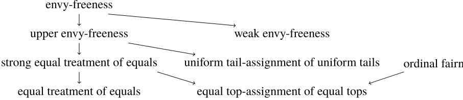
2.1 Relations between multiple fairness criteria . . . 41

3.1 Equivalence theorems . . . 50

3.2 Illustration of the chains I construct . . . 68

3.3 Steps 1, 2, and 3 . . . 71

3.4 Steps 4 and 5 . . . 72

A.1 Informational level-k model of BM . . . 79

A.2 Original Level-k model of BM in unbalanced markets . . . 80

A.3 Compare BM and DA in constrained school choice. . . 82

C.1 Illustration of Lemma 4. h1,h2are private endowments ofi1,i2. h3 is a social endowment. Hence, sh₁(t) = 2, si₁(t) = 3, sh₂(t) = 4, si₂(t)=5, andsh₃(t)=6. . . 92

C.2 Steps 1, 2, and 3 . . . 106

(10)

LIST OF TABLES

Number Page

1.1 Illustrating Example . . . 5

1.2 Procedures of BM and DA . . . 7

1.3 The original level-k reasoning process is analogous to the procedure of DA . . . 9

1.4 Informational level-k reasoning process of BM . . . 9

1.5 Example 1 . . . 17

1.6 Informational level-k model of BM in Example 1 . . . 18

1.7 The assignments of BM . . . 18

1.8 The rank distribution in BM and DA when(α, β)= (.4, .4) . . . 23

1.9 Average assignment rank at each level when(α, β)=(.4, .4) . . . 24

1.10 Percentage who prefer BM/DA at each level when(α, β)= (.4, .4) . . 24

1.11 Empirical estimation of the effect of replacing BM with DA . . . 27

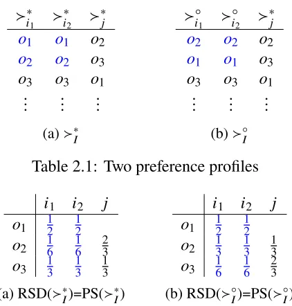
2.1 Two preference profiles . . . 33

2.2 The assignments for the two preference profiles . . . 33

3.1 The procedure of PSE in Example 2. . . 56

3.2 The procedure of PSE in Example 3 . . . 59

3.3 Example 4 . . . 64

3.4 Comparison betweenPSE and other mechanisms . . . 65

A.1 Counterexample . . . 83

B.1 Two preference profiles . . . 84

B.2 Pareto efficient assignments for both preference profiles . . . 84

B.3 ρ(∗_I) . . . 85

B.4 ρ(∗_I) . . . 85

B.5 ρ(◦_I) . . . 85

B.8 ρ(∗_I) . . . 88

B.9 ρ(◦_I) . . . 88

(11)

C h a p t e r 1

LEVEL-K REASONING IN SCHOOL CHOICE

1.1 Introduction

Many countries of the world provide public education, which allows students to attend schools for free. In the traditional system of K-12 public education in many countries, students are simply assigned to schools according to their home locations. This has been changed in the recent school choice trend: students (actually their parents) can submit their preferences over schools to a school choice office, then the office runs a computer algorithm to find an assignment. It is believed that the freedom of express preferences gives parents more control over their children’s education, and improves diversity in public schools. From the perspective of economics, a computer algorithm is a mechanism that maps the submitted preferences of students to an assignment. Therefore, school choice is a game for students.

There are two algorithms that are widely used in school choice: theBoston Mech-anismand thestudent-proposing deferred acceptance. BM is a status quo algorithm which has existed for a long time in many cities. DA is a new algorithm, which was first proposed by Gale and Shapley (1962) and then adapted by Abdulkadiroğlu and Sönmez (2003) to school choice. DA is strategy-proof, which means that reporting true preferences is a weakly dominant strategy for students. But BM is manipulable, which means that students may obtain better assignments by reporting non-truthful preferences. This difference motivates some cities to switch from BM to DA. A lot of studies compare the two algorithms and want to find which one produces a better assignment for students. However, a major difficulty is that the strategies used by students in BM have not been understood well. Field and lab evidence shows that students are often boundedly rational and have different abilities to manipulate BM. Specifically, some students do not realize that school choice is a game, so they always report true preference. The remaining may realize it, but some of them play better strategies than the others. Thus, the purpose of this paper is to explore the strategies used by students in BM when they have heterogeneous sophistication, and to compare the two algorithms.

(12)

(1995), and then developed by Ho, Camerer, and Weigelt (1998), Costa-Gomes, Crawford, and Broseta (2001), Costa-Gomes and Crawford (2006), Crawford and Iriberri (2007a,2007b), and Arad and Rubinstein (2012), among many others. The model shows a good explanatory power in many experiments. In the school choice game, the setup of the model is as follows. Every student has a discrete sophistication level, which is his depth of strategic reasoning. If a student’s level is zero, he is naive and does not make any strategic reasoning. If a student’s level is a positive integer k, he makes strategic reasoning and chooses a best strategy based on his belief about others’ levels. In the paper I consider two extreme settings of the beliefs of positive-level students. This consideration enables me to check the robustness of my results, and also examine the effect of beliefs on students’ strategies and welfare. In the first setting, a level-k student believes that all others are level-k-1 irrespective of their true levels. It is the setting commonly used in the literature, so I call the model with this settingoriginal level-k. In this setting a level-k student may overestimate some students’ levels and underestimate some others’. By contrast, in the second setting, I let students have as accurate beliefs as possible. However, the spirit of the level-k model requires that a level-k student cannot believe that any other’s level is k or higher.1 So in the second setting, any level-k student has a correct belief about the levels of those whose levels are lower than k, and believes the remaining are level-k-1. I call the corresponding model theinformational level-k.

Both DA and BM are preference revelation games. Since DA is strategy-proof, students report true preferences even though they have heterogeneous sophistication levels. So my main task in the paper is to use the two level-k models to analyze students’s strategies in BM. Hence, in BM level-0 students report true preferences, while positive-level students behave strategically. To study the problem in the most transparent environment, I assume a complete information environment. That is, students commonly know each other’s preferences and the priority rankings of students at all schools. Complete information is a widely used assumption in the matching theory literature. In this paper it removes the effect of probabilistic beliefs and risk attitudes on students’ strategies. So I can focus on the effect of heterogeneous sophistication. In the following I briefly discuss my main results.

First, in both level-k models of BM, when students reason about the others’ strategies, they essentially reason about the most preferred schools reported by the others. This is caused by the feature of BM that each school first admits those

1_{Otherwise, the level-k student should make more steps of reasoning and effectively has a level}

(13)

who report it as most preferred. Then I show that the reasoning process in both level-k models of BM is analogous to the procedure of DA. Specifically, when a positive-level student thinks about his best strategy, it is as if he runs some rounds of DA in his mind to decide which school he should report as most preferred; the higher is his level, the more rounds of DA he runs in his mind. I illustrate it in Section1.3through an example. Formal analysis is in Section1.4and Section1.5.

Second, I compare the assignments found by DA and BM. I find that in both level-k models the assignment found by BM is not strictly Pareto dominated by the assignment found by DA for any level distribution of students. Specifically, in both level-k models of BM a student always reports a school weakly better than his assignment in DA as most preferred. So it is impossible that all students obtain worse assignments in BM than in DA. When all students have levels above some thresholds defined in the paper, all students report their assignments in DA as most preferred. Hence, BM finds the same assignment as DA does. If I further make a mild assumption about the strategies of positive-level students, then I prove that the assignment of BM is never Pareto dominated by that of DA.

Last, I examine the effect of a student’s sophistication level and belief on his welfare in BM. This is to address the concern in practice that in BM, sophisticated students may take advantage of naive students and obtain better assignments. I find that in the original level-k model, a student of a higher level is not guaranteed to obtain a better assignment. It is because if a student has a higher level, he may overestimate more others’ levels and choose an overcautious strategy. By contrast, in the informational level-k model a student never overestimates the others’ levels. So when a student’s level is sufficiently high, he has a correct belief about the true levels of most others. Therefore, he can choose a truly best strategy. I show that students of sufficiently high levels must have weakly better assignments in BM than in DA. So in this sense they have advantage in BM. Moreover, the contrast between the two models shows that correct beliefs play a crucial role in the existence of the advantage.

(14)

latter, so more students prefer BM. To examine the effect of sophistication in BM, I look at the assignments of students at each sophistication level and compare them with those in DA. I find that the average assignment ofL0 students is worse than that of students of any positive level in BM, and is also worse than that ofL0 students in DA. By contrast, the average assignment of students of any positive level is better in BM than in DA. So this implies that in BM naive students have a disadvantage while sophisticated students have an advantage. But there is a difference between the two level-k models of BM. In the original level-k model the average assignment of students is single-peaked, while in the informational level-k model the average assignment of students is monotonic in their levels. Hence, correct beliefs are beneficial to students. My simulation results are similar in some respects to recent empirical studies of He (2014) and Calsamiglia, Fu, and Güell (2015). Both papers estimate that replacing BM with DA will hurt more students than helping them, and an average student be worse off. But they do not estimate the possible heterogeneous sophistication distribution among strategic students.

In the rest of the paper, I present the school choice model in Section1.2. Then I provide an example to illustrate BM and DA and the two level-k models in Section 1.3. The two level-k models of BM are in Section1.4and Section1.5. Section1.6 includes some discussions about models. Section1.7 presents simulation results. Section1.8 includes some extensions of the models. I discuss related literature in Section 1.9. Section 1.10 concludes. The appendix includes omitted proofs and additional results.

1.2 School Choice Model

A school choice problem consists of the following elements:

• a finite set of studentsI; • a finite set of schoolsS;

• a capacity vectorQS ={qs}s∈Swhereqs is the number of seats at schools; • a priority profile of schoolsΠS = {πs}s∈Swhereπsis the strict priority ranking

of schoolsover students;

(15)

There are enough seats to admit all students such that Í

s∈Sqs = |I|. This accommodates two cases. First, the law in many cities requires each student attend a public school, so it is natural to assume enough seats. Second, if students have outside options (private schools or studying at home), some school inSdenotes the outside options. Anassignmentof students to schools is a function µ: I →Ssuch that |µ−1(s)| ≤ qs for alls ∈ S. Here, µ(i)is the assignment of eachi and µ−1(s) is the set of students admitted by eachs. I denote the set of all assignments byM. A studenti justified enviesanother student j in an assignment µif µ(j)Piµ(i)and

iπµ(j)j. That is,i has a higher priority than j at school µ(j) buti is assigned to a school worse than µ(j). An assignment µiswasteful if |µ−1(s)| < qs and sPiµ(i) for somesand somei. That is,s has empty seats andiprefers sto his assignment. An assignment isstableif it does not contain justified envies and is not wasteful.

An assignment µPareto dominates another assignment µ0if µ(i)Riµ0(i)for all

i ∈ I, and µ(j)Pjµ0(j)for some j ∈ I. If µ(i)Piµ0(i)for alli ∈ I, µstrictly Pareto dominates µ0

. An assignment is Pareto efficient if it is not Pareto dominated by any other assignment. I use P to denote the set of all strict preference orderings of S, and use O to denote the set of all school choice problems. In practice ΠS is regulated and known by the school choice office. So throughout the paper I fix

I,S,QS,ΠS, and denote a school choice problem simply by PI. A school choice algorithm is a function ψ : O → M such that ψ(PI) is the assignment found for

PI. ψ isPareto efficientorstableifψ(PI)is Pareto efficient or stable for all PI. ψ isstrategy-proof if reporting true preferences is a weakly dominant strategy for all students. Formally, ψ(PI)(i) Ri ψ({P_i0,P−i})(i) for all i ∈ I, all PI ∈ P|I| and all

P_i0∈ P.

1.3 Illustrating Example

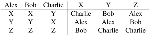
Consider a school choice problem that contains three students Alex, Bob, and Charlie, and three schools X, Y and Z. Each school has only one seat. Table1.1lists the preferences of students and the priority rankings at schools.

Alex Bob Charlie X Y Z

X X Y Charlie Bob Alex

Y Y X Alex Alex Bob

[image:15.612.177.433.605.667.2]

Z Z Z Bob Charlie Charlie

(16)

1.3.1 Procedures of BM and DA

In school choice each student is required to submit a list of schools, which is supposed to be his preference ordering, to an office. Then the office runs an algorithm to find an assignment. BM and DA are two most popular algorithms. They are run as follows. In the first round the applications of all students are simultaneously sent to the first schools in their reported lists, and schools tentatively admit applicants according to priority rankings. Then, the applications of rejected students are simultaneously sent to the next schools in their reported lists in the next round, and so on. BM and DA have a crucial difference since the second round: in BM once a school has no empty seats in some round, it cannot admit new applicants even though they have higher priorities than students admitted in earlier rounds; but in DA schools only consider the priority rankings of applicants without considering the timing of receiving their applications. It is well-known that DA always finds the student-optimal stable assignment, which Pareto dominates any other stable assignment. I denoted it by µD A.

The Procedures of BM and DA

Round 1: Each student applies to the first school in his reported list. Each school tentatively admits its applicants one by one according to its priority ranking until its all seats are occupied or all applicants are admitted. Remaining applicants, if any, are rejected. If all students are admitted, stop the procedure and finalize all assignments.

Roundr ≥ 2: Each rejected student applies to the next school in his reported list.

• In BM, each school with empty seats tentatively admits its applicants one by one according to its priority ranking until its all seats are occupied or all applicants are admitted. Remaining applicants, if any, are rejected. If all students are admitted, stop the procedure and finalize all assignments. • InDA, each school that receives new applications considers its earlier admitted

(17)

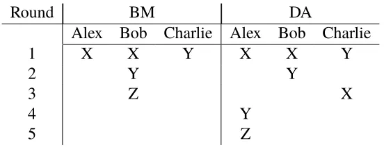
If all students in the example submit true preferences, Table1.2summarizes the procedures of BM and DA by listing the school that each student applies to in each round. In particular, although Bob has a higher priority than Charlie at Y, Bob loses his chance at Y in BM because he applies to Y in the second round while Charlie applies to Y in the first round.

Round BM DA

Alex Bob Charlie Alex Bob Charlie

1 X X Y X X Y

2 Y Y

3 Z X

4 Y

[image:17.612.169.445.168.276.2]

5 Z

Table 1.2: Procedures of BM and DA

In BM if a student ranks a school higher in his reported list, his application will be sent to the school in an earlier round. So in general when students want to manipulate BM, they often misreport their top ranked schools, especially their most preferred schools. In this example if Bob reports Y as first choice, he will be admitted by Y in BM.

1.3.2 Level-k Model of BM

I use two level-k models to analyze the strategies of students in BM in the complete information environment. In both models a level-0 student is naive and reports true preferences. In the original level-k model a level-k student for anyk > 0 believes others are level-k-1 and chooses a best strategy. In the informational level-k model a level-k student has a correct belief about the levels of those whose levels are lower than k and believes the remaining are level-k-1, then chooses a best strategy. The following presents the reasoning processes in the example.

1.3.2.1 Original Level-k Model of BM in the Example

• Level 0: If a student is level-0, he reports his true preferences in BM. In particular, he reports his most preferred school as first choice.

(18)

reports X as first choice. If it is Bob, in his best strategy Bob must report Y as first choice. Otherwise, he will not be admitted by X but also lose the chance at Y. If it is Charlie, in his best strategy Charlie must report Y as first choice. Otherwise, Charlie will be admitted by another school that he reports as first choice. However, for each student it is uncertain that how he reports the whole preference orderings in his best strategy.

• Level 2: If a student is level-2, he believes the others are level-1 and chooses a best strategy. In the complete information environment by conducting the above level-1 reasoning process in his mind, he knows the first choices reported by the others at level 1. Although he is uncertain about their whole reported preference orderings, it is sufficient for him to choose his best strategy in BM. If it is Alex, Alex knows that X is the school he wants to obtain by using a best strategy, and he can obtain X for sure by reporting it as first choice. So I assume that Alex just reports X as first choice.2 If it is Bob, in his best strategy Bob must report Y as first choice since he believes that Charlie also reports Y as first choice. If it is Charlie, in his best strategy he must report X as first choice. Otherwise, he will not be admitted by Y but also lose the chance at X. However, for each student it is still uncertain that how he reports the whole preference orderings in his best strategy.

• Level 3: If a student is level-3, he believes the others are level-2 and chooses a best strategy. In the complete information environment by conducting the above reasoning process in his mind, he knows the first choices reported by the others at level 2. If it is Alex, Alex knows that Z is the school he wants to obtain by using a best strategy, and he can obtain Z for sure by reporting it as first choice. So by my assumption Alex just reports Z as first choice. If it is Bob, Bob knows that Y is the school he wants to obtain by using a best strategy, and he can obtain Y for sure by reporting it as first choice. So by my assumption Bob just reports Y as first choice. If it is Charlie, in this best strategy Charlie must report X as first choice since he believes that Alex also reports X as first choice.

• Level k ≥ 4: If a student is level-4, he believes the others are level-3 and chooses a best strategy. In the complete information environment by

con-2_{If Alex believes that Charlie reports the preference ordering of}_Y _Z _X_{at level 1, he believes}

(19)

ducting the above reasoning process in his mind, he knows the first choices reported by the others at level 3. By my assumption Alex still reports Z as first choice, Bob still reports Y as first choice, and Charlie still reports X as first choice. It is easy to see that same conclusions also apply to all levels higher than 4.

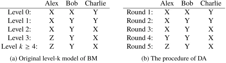
There are two observations from the above procedure. First, in the reasoning process a level-k student essentially reasons about the first choices reported by the others at level k-1. Second, by looking at the first choices reported by students, the level-k reasoning process is analogous to the procedure of DA. I illustrate it by Table 1.3. For each round of DA and each student, the school I list is the school admitting

the student in the previous round, or the school the student applies to in the round. Alex Bob Charlie

Level 0: X X Y

Level 1: X Y Y

Level 2: X Y X

Level 3: Z Y X

Levelk ≥ 4: Z Y X

(a) Original level-k model of BM

Alex Bob Charlie

Round 1: X X Y

Round 2: X Y Y

Round 3: X Y X

Round 4: Y Y X

Round 5: Z Y X

[image:19.612.118.493.297.403.2]

(b) The procedure of DA

Table 1.3: The original level-k reasoning process is analogous to the procedure of DA

1.3.2.2 Informational Level-k Model of BM in the Example

In the informational level-k model a positive-level student’s strategy depends on the levels of those whose levels are lower than him. Hence, I assume a level distribution: Alex is level-1, Bob is level-0, and Charlie is level-2. As before, in the reasoning process students essentially reason about the first choices reported by the others. So Table1.4lists the first choices reported by students at each level.

Alex Bob Charlie

Level 0: X X Y

Level 1: X Y

Level 2: Y

Table 1.4: Informational level-k reasoning process of BM

[image:19.612.226.386.591.649.2]

(20)

level-1, so he would report X as first choice and obtain it. So Charlie obtains a better assignment by having a correct belief. In the paper I show that the level-k reasoning process in this model is also analogous to the procedure of DA. But correct beliefs of high-level students can bring them better assignments.

1.4 The Original Level-k Model of BM

From now on if a student is level-k, I simply say he isL k. In the original level-k model L0 students report true preferences. An L k student for any k > 0 believes the others areL k−1. In the main content of this paper, I assume that the preference profile and priority rankings are common knowledge among students. Under this assumption eachL kstudent can infer others’ strategies at lower levels, then chooses a best strategy at his level. I call the school an L k student wants to obtain by reporting a best strategythe best obtainable school at L k for him. In general, best strategies are not unique. In particular, any preference ordering that lists the best obtainable school at L k as first choice is a best strategy. In this paper I make the assumption that an L k student always reports his best obtainable school at L k as first choice, and this is common knowledge among all positive-level students.

Best strategy selection assumption: AnL k student for anyk > 0 reports his best obtainable school atL k as first choice, and this is commonly known by students at positive levels.

In the illustrating example of Section1.3, an L kstudent often has to report his best obtainable school at L k as first choice in his all best strategies. This happens when he believes that there are enough many other student who also report his best obtainable school atL kas first choice, and when he believes that if he reports another school as first choice, he must obtain it. In Section 1.6.3I discuss the validity of this assumption. For most results of the paper I do not assume how positive-level students report the whole preference orderings. This not only make my results robust to any further assumption, but also captures the uncertainty of students in the level-k reasoning process about the others’ whole reported preference orderings.

By slightly adjusting the procedure of DA, I prove that the reasoning process in the original level-k model of BM can be understood through the adjusted procedure. Formally, I use s_ik to denote the school each studenti reports as first choice at any

(21)

any schoolsthat has admittedqs students each of whom has a higher priority than him ats. Fast DA always find the same assignment as DA.

Fast Deferred Acceptance

Roundr ≥ 0: Each unassigned studentiapplies to his most preferred schoolsthat he has not applied to and has not admittedqsstudents who all have higher priorities thaniats. Each school tentatively admits students according to its priority ranking. If all students are admitted after this round, stop the procedure.

Note that I index the first round of Fast DA by 0. I denote the last round of Fast DA byrF D A. Then for eachiand eachk ≥ 0 I define

a_ik ≡           

the school admittingiin round k−1, ifiis admitted in roundk −1, the schooliapplies to in roundk, ifiis rejected in roundk −1,

ar_iF D A, ifk >rF D A.

That is,a_ik is the school that admitsiin roundk −1 of Fast DA, or the schooli

applies to in round k. If k > rF D A, a_ik is the school that finally admitsi, which is justµD A(i). Now I prove thata_ikis exactly the school eachireports as first choice at anyL kof the original level-k model of BM. So it is as if students run the procedure of Fast DA in their minds to do their level-k reasoning.

Proposition 1. For anyPI,s_ik =a_ik for alliand all k ≥ 0.

Proposition 1 implies that each i must report a weakly worse school as first choice at a higher level, but the school is no worse than µD A(i).

Corollary 1. For anyPI and anyi,

(1)s_ik Ri s_ik+1 Ri µD A(i)for allk ≥ 0;

(2) there exists some finite ri ≥ 0 such that s_ik Pi µD A(i) for all k < ri, and

s_ik = µD A(i)for allk ≥ ri.

(22)

strategies such thati’s best strategy is to cautiously report a weakly worse school as first choice. However, since students compete with each other only through priority rankings in DA, the situation in DA is weakly more competitive than all possible situation in BM. Hence,i’s reported first choice in BM is never worse thanµD A(i).

1.4.1 Efficiency Comparison between BM and DA

I usekito denote anyi’s level and usekI ≡ {ki}i∈Ito denote any level distribution. If ki ≥ ri (the threshold defined in Corollary1),i reports µD A(i)as first choice no matter how high ki is. So I sayi issufficiently sophisticated. If ki < ri, I sayi is insufficiently sophisticated. I use µBM_k

I to denote the assignment of BM for anyPI

when the level distribution iskI.

Although I do not characterize the whole preference orderings reported by positive-level students, characterizing their reported first choices is sufficient for me to make some comparison betweenµBM_k

I andµ

D A_{. Specifically, in the first round} of BM there must be some students who are admitted by their reported first choices. By Corollary 1, for any i who is admitted by his reported first choice s, if i is insufficiently sophisticated, smust be strictly better than µD A(i); ifi is sufficiently sophisticated,smust coincide with µD A(i). So I have the following proposition.

Proposition 2. For anyPI:

1. µBM

kI is not strictly Pareto dominated byµ

D A_{for any}

kI;

2. If each student is sufficiently sophisticated,µBM kI = µ

D A_;

3. If each student is insufficiently sophisticated,µBM

kI is not Pareto dominated by

µD A_.

So µD A can Pareto dominate µBM_k

I only when some students are insufficiently

sophisticated while the others are sufficiently sophisticated. In the following I prove that if that happens, there must be some insufficiently sophisticated studenti who prefers µD A(i)to µBM_k

I (i)but reports that µ

BM

kI (i)is preferred to µ

D A₍_i₎_.

Lemma 1. For anyPI and any kI, ifµD APareto dominates µBM_k

I , there exists some

insufficiently sophisticated studentiwho reports someP_i0such thatµBM_k I (i)P

0 i µ

D A₍_i₎_, but µD A₍_i₎_P

i µBM_k

(23)

So if each insufficiently sophisticated studenti reports the truthful preferences between µD A(i)and any school worse than µD A(i), then µBM_k

I is never Pareto

domi-nated byµD A.

Proposition 3. For anyPI and anykI, if each insufficiently sophisticated studenti reports a best preference ordering P_i0such that µD A(i)Pi simplies µD A(i) P_i0s for anys ∈S, thenµBM_k

I is not Pareto dominated by µ

D A_.

There is a simple best strategy P_i0 for each insufficiently sophisticated i that satisfies the above condition: i only manipulates his first choice and reports the truthful preference ordering of the remaining schools. Formally, ifireportssas first choice, thensP_i0s0for alls0, s, and s0Pi0s

00 _{if and only if}

s0Pis00 for alls0,s00 , s. I callP_i0atopping strategy.

For anyPI, I call the ordering of the schools that anyiapplies to in the procedure of Fast DA theexpressed preferences ofi in Fast DA. If µD Ais not Pareto efficient with respect to the expressed preferences of students in Fast DA, there exists a level distributionkIsuch that all students obtain their reported first choice andµBM_k

I Pareto

dominatesµD A.

Proposition 4. For anyPI, ifµD Ais not Pareto efficient with respect to the expressed preferences of students in Fast DA, then there exists some kI such that µBM_k

I Pareto

dominates µD A_.

1.4.2 Advantage of Sophisticated Students in BM

A popular concern in practice about BM is that a student may obtain a better assignment if he is more sophisticated. It is easy to show that this concern does not hold in general in the original level-k model of BM. It is because a student of a higher level may overestimate others’ levels such that he chooses an overcautious strategy. For example, in the example of Section1.3if all students are level-0, Alex is admitted by X and Bob is admitted by Z. If Bob becomesL1, Bob is admitted by Y and becomes better off. But if Alex becomes level-3, Alex is admitted by Z and becomes worse off.

1.5 The Informational Level-k Model of BM

In the informational level-k model an L k student for any k > 0 has a correct belief about the level of any L k0student if k0 < k, and believes the remaining are

(24)

this section I use ˜s_ik(kI) to denote the first choice reported by anyi at L k for any 0 ≤ k ≤ ki. Interestingly, the level-k reasoning process in this model can still be understood through an adjusted procedure of DA. Formally, for any PI and anykI, I define:

Fast Deferred Acceptance∗

Roundr ≥ 0: For each unassigned studenti, ifki ≥r, theniapplies to her most preferred schoolsthat he has not applied to and has not admittedqsstudents who all have higher priorities thaniats. Each school tentatively admits students according to its priority ranking. If ki < r for all unassigned i, or all students are admitted after this round, stop the procedure.

Fast DA∗is different from Fast DA in that an unassignedicannot apply to a new school in any roundr > ki. Since its procedure depends onkI, I denote its outcome by µF D A_k ∗

I . If some i is unassigned in µ

F D A∗

kI , I say i is admitted by ∅. Letr

F D A∗ kI

denote the last round of Fast DA∗. Then for eachi and each 0≤ k ≤ kiI define:

˜

a_ik(kI) ≡             

the school admittingiin round k−1, ifiis admitted in roundk −1, the schooliapplies to in roundk, ifiis rejected in roundk −1,

˜

ar F D A∗ kI

i , ifk >r F D A∗ kI .

Proposition 5. For anyPI and any kI,s˜_ik(kI)= a˜_ik(kI)for alliand all0≤ k ≤ ki.

By definition ˜aki

i (kI)is the last school that eachiapplies to in Fast DA

∗_{. It is also} the first choice reported by eachiin BM. So µF D A_k ∗

I coincides with the assignment

found by the first round of BM.

Corollary 2. For any PI and any kI, µF D A ∗

kI is the assignment found by the first

round of BM.

If all students are sufficiently sophisticated, eachimust finally apply to µD A(i)in Fast DA∗. ThenµF D A_k ∗

I coincides withµ

D A_{. If some}

iis insufficiently sophisticated, since he applies to fewer schools than being sufficiently sophisticated, some other

(25)

Fast DA∗.3 If all students are insufficiently sophisticated, eachi must finally apply to a school better than µD A(i)in Fast DA∗. So I have the following corollary.

Corollary 3. For anyPI,

(1) for any kI,s˜_ik(kI)Ri s˜_ik+1(kI)Ri µD A(i)for alliand all0 ≤ k ≤ ki; (2) if each student is sufficiently sophisticated, µF D A∗

kI = µ

D A_;

(3) if each student is insufficiently sophisticated,s˜ki

i (kI)Pi µ

D A₍_i₎_{for all}_i_.

1.5.1 Efficiency Comparison between BM and DA

For anyPI and anykI, I denote the assignment of BM by ˜µBM_k

I . Using Corollary

3I can prove the following result in the same way as in the previous section.

Proposition 6. For anyPI:

1. µ˜BM_k

I is not strictly Pareto dominated byµ

D A_{for any}

kI;

2. If each student is sufficiently sophisticated,µ˜BM_k

I = µ

D A_;

3. If each student is insufficiently sophisticated,µ˜BM_k

I is not Pareto dominated by

µD A_;

4. If each positive-levelireports a best strategyP_i0such that µD A(i)Pisimplies

µD A₍_i₎_P0

i sfor anys ∈ S, then µ˜ BM

kI is not Pareto dominated by µ

D A_{for any}

kI.

There is no counterpart of Proposition 4 in this section because if all students obtain their reported first choice, ˜µBM_k

I coincides with µ

D A_.

1.5.2 Advantage of Sophisticated Students in BM

To investigate the advantage of sophisticated students in BM, I compare the assignment of BM when j is L kj with the assignment of BM when j is L k0_j for any k0_j > kj. Since I only characterize the first choices reported by students, I investigate how the assignment found by the first round of BM changes when j’s level is increased from L kj to L k0_j for any k0_j > kj. By Corollary2it is equivalent to investigating how the outcome of Fast DA∗changes. My first result is as follows.

3_{In particular, even though}_j_{is sufficiently sophisticated, if his level is not high enough,}_i_{can be}

unassigned in Fast DA∗. This is different from the previous model in which a sufficiently sophisticated

(26)

Proposition 7. For any PI and any kI, if any j ∈ I becomes L k0_j for any k0_j > kj, then,

• if µF D A∗

kI (j),∅, µ˜

BM kI = µ˜

BM (k0

j,k−j);

• if µF D A∗

kI (j)=∅, for anyi ∈I such thatµ

F D A∗

kI (i), ∅and µ

F D A∗ (k0

j,k−j)

(i)_, ∅:

– ifki ≤ kj+1, µ˜BM_k

I (i)= µ˜

BM (k0

j,k−j)

(i);

– ifki > kj+1, µ˜BM_k

I (i) Ri µ˜

BM (k0_j,k−j)(i).

The proof is as follows. If j is assigned in µF D A_k ∗

I , it means that j obtains his

reported first choice. Then becoming L k0_j does not change j’s strategy as well as the others’. So the outcome of BM does not change. If j is unassigned in µF D A_k ∗

I ,

then by becoming L k0_j, jwill apply to more schools in Fast DA∗than before. Then for anyi such that µF D A_k ∗

I (i), ∅andµ

F D A∗ (k0

j,k−j)

(i)_, ∅, if ki ≤ kj +1, the level change of jcannot affect the set of schools thatiapplies to in Fast DA∗. Soi’s assignment does not change. If ki > kj +1, since j applies to more schools than before in in Fast DA∗,i will also apply to weakly more schools than before. Soi’s assignment must be weakly worse off.

For any PI, define ¯r ≡ maxkIr

F D A∗

kI . That is, ¯r is the largest last round of Fast

DA∗for all possiblekI.4 If anyi’s level is weakly higher than ¯r,imust be assigned in the outcome of Fast DA∗ irrespective of the others’ levels. So I sayi is quasi-rationalifki ≥ r¯. A quasi-rational student is sophisticated enough in the sense that he always obtains his reported first choice. For any PI and any kI, I denote the set of quasi-rational students by M and the set of the remaining by N. Proposition 7 implies the following corollary.

Corollary 4. For anyPIand anykI, ifM , ∅andN , ∅, then if anyj ∈Nbecomes

L k0_j for anyk0_j > kj,

˜

µBM

kI (i)Ri µ˜

BM (k0

j,k−j)

(i)for alli ∈ M.

If all students inNbecome quasi-rational, the outcome of Fast DA∗will coincide with µD A. Then Corollary4implies the following result.

Corollary 5. For any PI and any kI, if M , ∅, all students in M obtain weakly better assignments in BM than in DA.

(27)

For any kI, define ¯kN ≡ maxi∈N ki. If M = ∅ and there exists a unique Lk¯N studenti,imust be assigned in µF D A_k ∗

I and obtains an assignment weakly better than

µD A₍

i). It is because no students other thani can apply to schools in round ¯kN of Fast DA∗. Then ifi is assigned in round ¯kN −1, i must still be assigned in round

¯

kN; ifi is unassigned in round ¯kN −1,i must apply to a school in round ¯kN and is admitted. So Proposition7implies the following corollary.5

Corollary 6. For anyPI and any kI, ifM = ∅and there is a uniqueLk¯N studenti, (1) if any j ∈ N\{i}becomesL k0_j for anykj < k0_j < ki, µ˜BM_k_I (i) Ri µ˜_(kBM0

j,k−j)

(i); (2)i obtains a weakly better assignment in BM than in DA.

If µF D A_k ∗

I (j) = ∅, j may not be better off by becoming more sophisticated. It is

shown by the following example. It is because the other students in N who have higher levels than jmay respond to the level change of j by using more competitive strategies.

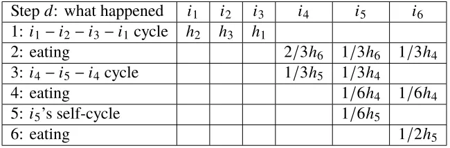
Example 1. I = {i1,i2,i3,i4,i5,i6} and S = {s1,s2,s3,s4,s5,s6}. Each school has

one seat. The preferences of students and the priority rankings of schools are shown in Table1.5.

Pi1 Pi2 Pi3 Pi4 Pi5 Pi6 πs1 πs2 πs3 πs4 πs5 πs6

s1 s2 s3 s4 s1 s1 i6 i3 i4 i5 i2 ...

s2 s1 s2 s3 s4 ... ... i1 i3 i4 i1

s5 s3 ... ... ... i2 ... ... ...

s6 s5 ...

... ...

Table 1.5: Example 1

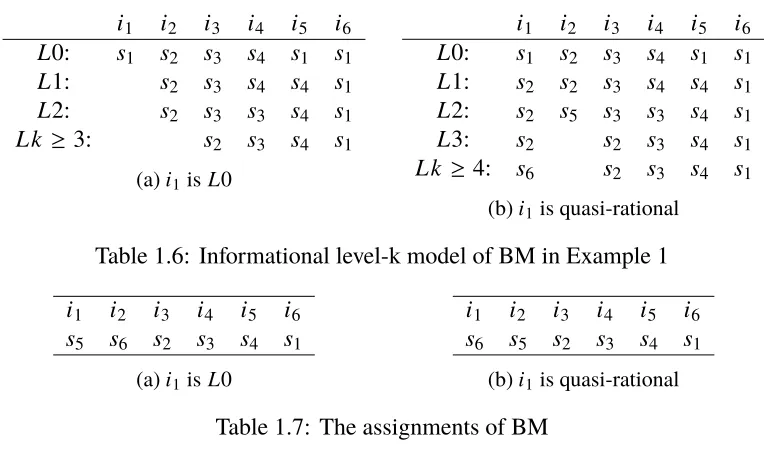
Supposei1 is L0, i2is L2, and all others are quasi-rational. The first choices

reported students are shown in Table 1.6a. If i1 becomes quasi-rational, the first

choices reported by students are shown in Table1.6b.

If all positive-level students use topping strategies, then the outcomes of BM are shown in Table1.7. It is easy to see thati1is worse off by becoming quasi-rational.

However, if j has the highest level among N, I prove that j must be weakly better off by becoming more sophisticated and using a strategy that satisfies a mild

5_{If there are multiple}_L_k_¯

(28)

i1 i2 i3 i4 i5 i6

L0: s1 s2 s3 s4 s1 s1

L1: s2 s3 s4 s4 s1

L2: s2 s3 s3 s4 s1

L k ≥3: s2 s3 s4 s1

(a)i1isL0

i1 i2 i3 i4 i5 i6

L0: s1 s2 s3 s4 s1 s1

L1: s2 s2 s3 s4 s4 s1

L2: s2 s5 s3 s3 s4 s1

L3: s2 s2 s3 s4 s1

L k ≥ 4: s6 s2 s3 s4 s1

[image:28.612.115.497.67.292.2]

(b)i1is quasi-rational

Table 1.6: Informational level-k model of BM in Example 1

i1 i2 i3 i4 i5 i6

s5 s6 s2 s3 s4 s1

(a)i1isL0

i1 i2 i3 i4 i5 i6

s6 s5 s2 s3 s4 s1

(b)i1is quasi-rational

Table 1.7: The assignments of BM

condition. Formally, I usePk_jj and Pk

0

j

j to denote the preference orderings reported by j at L kj and L k0_j respectively. If s is the first choice in P

k0_j

j , I say P k0_j

j satisfies worse-rank invarianceif for anys0such thatsPjs0,s0has the same rank inP

kj j and Pk 0 j j .

Proposition 8. For any PI and any kI, if any j ∈ N of kj = k¯N becomes L k0_j for anyk0_j > kj and his strategy satisfies worse-rank invariance, then

˜

µBM (k0

j,k−j)

(j)Rj µ˜BM_k_I (j).

If j uses topping strategies at both L kj and L k0_j, the worse-rank invariance condition is satisfied. If j becomes quasi-rational, since j must be admitted by his reported first choice, j is weakly better off even if his strategy does not satisfy worse-rank invariance.

1.6 Discussion

1.6.1 Insights from the Two Level-k Models

[image:28.612.116.499.72.164.2]

(29)

they may overestimate others’ levels, while in the informational level-k model a student has a definite advantage in BM only when his level is high enough relative to the others. Hence, the two model together imply that both high sophistication and accurate belief are crucial for a student to have any advantage in BM.

1.6.2 Comparison with Nash Equilibrium Models

It is interesting to compare my results with those of Nash equilibrium models in the complete information environment. By assuming all students are rational, Ergin and Sönmez (2006) prove that every NE outcome of BM is a stable assignment with respect to true preferences of students. Since DA always finds the student-optimal stable assignment, it implies that BM is weakly Pareto dominated by DA. However, in the two level-k models if students are sufficiently sophisticated, BM finds the same assignment as DA. Hence, when students are very sophisticated and are more likely to use the level-k reasoning than using the circular equilibrium reasoning, students are more likely to coordinate on the stable-optimal stable assignment.

Pathak and Sönmez (2008) use a NE model to show that rational students can take advantage of naive students in BM. In their model students are either rational and naive, and rational students commonly know the identifies of naive students. By assuming that the best NE outcome of BM is always realized, they prove that there exists a conflict of interest between naive students and rational students. In particular, rational students obtain weakly better assignments in BM than in DA. This dichotomous sophistication distribution can be seen as a special case of my models. Indeed, I prove that if students are either L0 or quasi-rational, then the outcome of BM in the informational level-k model is exactly the best NE outcome in the BM game whereL0 students are naive and quasi-rational students are rational. Then the results of Pathak and Sönmez are corollaries of mine.

Proposition 9. For any PI and any kI, if N,M , ∅ and kN = 0, then µ˜BM_k_I is the best NE outcome in the BM game whereN are naive andM are rational.

In Appendix A.2 I use a new method to characterize the set of NE outcomes of BM when N are naive and M are rational. Proposition9 is a corollary of the characterization (Proposition 15). Then by Proposition 7 if any j ∈ N becomes quasi-rational, all students in M are weakly worse off in BM. Since kN = 0, each

(30)

of Pathak and Sönmez.6

Abdulkadiroğlu, Che, and Yasuda (2011) analyze a special incomplete informa-tion environment in which schools do not prioritize students and students share a common ordinal preference ordering over schools (but may have different cardinal utilities). They prove that in any symmetric Bayesian NE of BM students have weakly higher utilities in BM than in DA, and if there exist naive students, they can benefit from the equilibrium strategies of rational students.7 I want to argue that the driving force behind their result is the special priority and preference assump-tion, not the incomplete information environment. Specifically, in the no priorities environment any two students of same cardinal utilities are assumed to play same strategies and also treated equally by schools. So when a rational student calculates his best strategy, he does not need to know the identities of others if he knows the distribution of cardinal utilities in the student population. Hence, assuming com-mon knowledge of the cardinal utility distribution in the incomplete information environment is similar to assuming complete information. In Section1.8I provide a preliminary analysis of a level-k model of BM in the incomplete information environment.

1.6.3 Validity of My Assumptions about Students’ Strategies

L0strategy Intuitively,L0 strategy captures the instinct response of a player to a game. Since school choice is a preference revelation game, I believe my assumption that L0 students report true preferences is valid. In other games such as “p-beauty contest”,8 there is no natural focal point for L0 players, so it is often assumed L0 players use a random strategy.9

6_{In Appendix}_A.2_{I show that the other results of Pathak and Sönmez are also proved easily by} my method.

7_{Abdulkadiroğlu, Che, and Yasuda (}₂₀₁₁_{) also consider the complete information environment} with strict priorities. They prove that if any naive student becomes rational, the other naive students must be weakly worse off in the unique NE outcome of BM. So naive students suffer from the existence of rational students. In AppendixA.5I show that this result is actuallyincorrect.

8_{In the game each player is asked to propose an integer between 0 and 100. The winner is the}

one whose proposal is closest to a multiplepof the group average.

9_{In some games it is believed that some strategies are more likely to become instinct responses}

than the others. In the literature they are calledsalient strategies. For example, Crawford and Iriberri (2007a) point out the framing effects in the experiments of “hide-and-seek” games. By suitably adapting L0 behavior to salient strategies, they show that the level-k model can well explain the

experimental dataset. Arad and Rubinstein (2012) conduct experiments of the “11-20” game to

(31)

L kstrategy I assume that anL kstudent for anyk > 0 report their best obtainable schools as first choice. In many situations students have to do that in their best strategies. In other situations I believe my assumption is still reasonable. First, because first choice plays the most important role in determining a student’s assign-ment in BM, it is natural that students are attracted to focus on first choice. This is supported by lab evidence. In the experiment of Chen and Sönmez (2006), 70.8% of students receive their reported first choices in BM, but only 28.5% receive their true first choices. So over 40% of students manipulate and obtain their first choices. Second, in practice students may be advertised/convinced to focus on first choice. For example, Boston provided a reference material to students in 2004 that sug-gested students to strategically choose their first choices. In Seattle and Tampa-St. Petersburg similar suggestions appear in local press (Abdulkadiroğlu et al. 2005). Last, as illustrated in the example of Section 1.3, in the level-k reasoning process students are often uncertain about the whole preferences reported by others at lower levels. If students is risk-averse and considers the worst case, they should assume that others optimally manipulate their first choices. Then my assumption captures such worst-case consideration.

1.7 Simulation

In previous sections I allow the level distribution to be arbitrary. But many experiments have found that subjects’ levels are often not high. So in this section I do simulations by randomly generating students’ levels from a reasonable distribution.

1.7.1 Setup

There are 1000 students and 20 schools. Each school has 50 seats. Although my models do not involve in utilities, I randomly generate the utilities of students and schools to generate preferences and priority rankings. Formally, the utility function of each studentiis denoted byUiand the utility function of each schoolsis denoted by Us. Each utility consists of a private-value component and a common-value component:

Ui(s) ≡ αU(s)+(1−α)i(s),

Us(i) ≡ βU(i)+(1−β)s(i),

(32)

from the uniform distribution on [0,1]. α, β ∈ [0,1] are correlation coefficients. In my simulation I vary the values of α, β from 0 to 1 in steps of .2. So α, β ∈ {0, .2, .4, .6, .8,1}. Students’ preferences and schools’ priority rankings are generated as:

Pi :sa Pi sb ⇔ Ui(sa)>Ui(sb),

πs :ia πs ib ⇔ Us(ia)> Us(ib).

For every value pair of (α, β) I randomly generate 1000 markets. In each market I draw the levels of students independently and identically from the Poisson distribution with a mean of 2. This distribution is consistent with the estimation of level distribution in multiple experiments.10 In particular, in this distribution the probabilities for L0 toL4 are respectively .135, .271, .271, .180, .090.

In previous sections I do not assume how positive-level students report whole preferences. In the simulation I consider two strategy settings. In the first setting positive-level students use topping strategies. That is, they report true preferences over the schools other than reported first choices. In the second setting they report random preference orderings over the schools other than reported first choices which are independently and identically drawn from the uniform distribution. I call them random strategies. The two settings enable me to check the robustness of simulation results.

1.7.2 Result

There are 36 pairs of(α, β). For convenience I first report the simulation results corresponding to(α, β)= (.4, .4). The results for other pairs are similar. To measure the welfare of students in BM and DA, I calculate the ranks of their assignments in their true preferences. Table1.8reports the rank distribution and the average rank in the two level-k models of BM with the counterparts in DA, as well as the percentage of students that obtain better assignments in BM and the percentage of students that obtain better assignments in DA.

There are three observations from Table1.8. First, the rank distributions in the two level-k models of BM are very close, and the difference between the topping strategy setting and the random strategy setting is small. Second, BM produces

(33)

Rank BM (%)

(topping)

BM (%)

(random)

DA (%)

1 25.72 25.62 > 18.44

2 18.02 17.55 > 15.77

3 13.93 12.30 < 13.24

4 10.65 9.35 < 11.11

5 8.04 6.71 < 9.35

6 6.08 4.82 < 7.81

7 4.46 3.53 < 6.27

8 3.27 2.64 < 4.91

9 2.40 2.01 < 3.71

10 1.71 1.62 < 2.72

11 1.27 1.36 < 1.95

12 .95 1.21 < 1.41

13 .72 1.10 < 1.03

14 .59 1.05 < .75

15 .46 1.03 < .53

16 .40 1.08 > .38

17 .34 1.18 > .27

18 .30 1.36 > .18

19 .29 1.66 > .11

20 .40 2.13 > .05

Avg rank 4.0 4.9 4.6

Topping:32.8%prefer BM>12.6%prefer DA

Random: 30.7%prefer BM>18.2%prefer DA (a) Original level-k

Rank BM (%)

(topping)

BM (%)

(random)

DA (%)

1 26.44 26.07 > 18.44

2 18.36 17.85 > 15.77

3 14.00 12.92 < 13.24

4 10.54 9.00 < 11.11

5 7.77 6.13 < 9.35

6 5.73 4.21 < 7.81

7 4.18 2.95 < 6.27

8 3.11 2.26 < 4.91

9 2.31 1.84 < 3.71

10 1.70 1.57 < 2.72

11 1.28 1.40 < 1.95

12 .98 1.29 < 1.41

13 .75 1.24 < 1.03

14 .61 1.20 < .75

15 .50 1.23 < .53

16 .42 1.29 > .38

17 .35 1.42 > .27

18 .30 1.63 > .18

19 .29 1.99 > .11

20 .38 2.51 > .05

Avg rank 4.0 5.1 4.6

Topping: 35.1%prefer BM>14.1%prefer DA

Random:32.5%prefer BM>21.1%prefer DA (b) Informational level-k

Table 1.8: The rank distribution in BM and DA when(α, β)=(.4, .4)

more extreme assignments than DA: in BM more students obtain high or low-ranked assignments, while in DA more students obtain medium-ranked assignments. Third, although the comparison between the average ranks in BM and DA depends on the two strategy settings, there are always more students who prefer BM than those who prefer DA. So neither BM nor DA dominates the other, but more students prefer BM.

Result 1. For(α, β)=(.4, .4):

1. The rank distribution in BM and DA does not depend on the two level-k models and the two strategy settings;

2. BM produces more extreme assignments than DA;

(34)

Level Average rank of assignments

Original level-k of BM Informational level-k of BM DA topping random topping random

0 6.0 6.6 6.0 6.5 4.59

1 4.5 6.9 4.5 7.2 4.58

2 3.2 3.8 3.1 3.3 4.59

3 3.2 3.2 2.94 3.0 4.59

4 3.6 3.6 2.94 3.0 4.59

5 3.9 3.9 2.93 2.97 4.60

[image:34.612.135.485.67.223.2]

... ... ... ... ... ...

Table 1.9: Average assignment rank at each level when(α, β)= (.4, .4)

Level Prefer BM|DA (%)

Original level-k of BM Informational level-k of BM topping random topping random 0 19.97|41.19 17.11|45.41 19.53|41.39 16.75|45.39 1 31.19|21.15 26.52|36.00 29.18|22.23 23.78|38.68 2 42.20|4.55 40.84|8.45 38.66|7.82 36.44|14.49 3 37.16|.06 37.16|.09 43.03|1.61 42.66|2.87 4 27.62|≈0 27.50|≈0 44.06|.17 43.78|.26 5 21.00|≈0 20.33|≈0 44.47|≈0 44.11|≈0

... ... ... ... ...

Table 1.10: Percentage who prefer BM/DA at each level when(α, β)=(.4, .4) To examine how a student’s welfare depends on his sophistication level, for the students at each level from L0 to L5, in Table 1.9 I report the average rank of their assignments in BM and DA, while in Table 1.10 I report the percentage of students who obtain better assignments in BM and the percentage of students who obtain better assignments in DA. In DA, the average rank for all levels is almost always 4.59, but in BM the average rank depends on level. In particular, in BM the average rank for level-0 students in BM is lower than the average rank for any positive-level students, and is also lower than the average rank in DA. By contrast, positive-level students have higher average ranks in BM than in DA. Similar can also be observed from Table1.10: among level-0 students more prefer DA, while among positive-level students more prefer BM.

However, Table 1.9 shows an important difference between the two level-k models. In the original level-k model the average rank in BM has a single peak at

[image:34.612.144.471.264.419.2]

(35)

largest number of students’ levels. By contrast, in the informational level-k model the average rank increases in level. So higher-level students on average obtain better assignments. This is similarly observed in Table1.10. So I have the following result.

Result 2. For(α, β)=(.4, .4):

1. Level-0 students are on average better off in DA, while positive-level students are on average better off in BM;

[image:35.612.115.523.258.580.2]

2. The advantage of positive-level students is single-peaked in the original level-k model of BM, but increases in level in the informational level-k model of BM.

Figure 1.1: Simulation results in original level-k

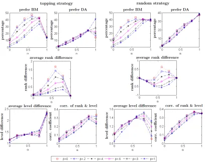
Figure1.1summarizes the simulation results for all pairs of(α, β)in the original level-k model. The simulation results for the informational level-k model are almost same and reported in Appendix A.3.11 There are five subfigures for each strategy

(36)

setting. In each subfigure the horizontal axis is the value of α, and the six lines correspond to the six values of β. For most pairs of(α, β), there are more students who prefer BM than those who prefer DA.₁₂ Average rank difference is equal to the average rank of all students’ assignments in DA minus the average rank of all students’ assignments in BM. I use it to compare the average welfare of students in BM and DA. If it is positive, students are on average better off in BM; vice versa. When topping strategies are used, students are on average better off in BM for all pairs of(α, β),13while when random strategies are used, the answer depends on the pairs of (α, β). So in general it is uncertain that which algorithm gives students a higher average welfare. The last two subfigures examine the advantage of sophisticated students in BM. Average level difference is equal to the average level of those who prefer BM minus the average level of those who prefer DA. In the figure it is always positive. Corr. of rank & level reports the correlation coefficient between the preference ranks of students’ assignments in BM and their levels. In the figure it is always positive and significantly above zero for most pairs of(α, β). Hence, both subfigures suggest that positive-level students have advantage in BM.

Result 3. For all pairs of(α, β):

1. There are more students who prefer BM than those who prefer DA;

2. Positive-level students have advantage in BM.

1.7.3 Comparison with Empirical Estimation

It is interesting to compare my simulation results with recent empirical esti-mations conducted by He (2014) and Calsamiglia, Fu, and Güell (2015). He uses the dataset from Beijing of China, and Calsamiglia et al. use the dataset from Barcelona of Spain. Both cities implemented some kind of BM in their school choice programs. The two studies accommodate the fact that students have het-erogeneous sophistication types. After estimating the preferences of students they

students’ preferences and plays the role of “unassigned”. Unbalanced markets make some of the simulation results sharper, but my qualitative conclusions do not change.

12_α₌_{1 in the topping strategy setting is an exception. It is because when}_α₌_{1 students have} identical preferences, and by using topping strategies they report highly correlated preferences in BM. So the assignment in BM is mainly determined by priority rankings of schools, which is further

determined by β. By contrast, in the random strategy setting students report weakly correlated

preferences.

(37)

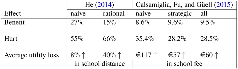
conduct counter-factual analyses to predict the effect of replacing BM with DA in the two cities. Specifically, He develops an approach to estimate the preferences of students without having to estimate their sophistication distribution. In his counter-factual analysis he only considers the welfare of naive students and rational students. Calsamiglia et al. estimate both the preferences of students and their sophistication types. But they assume that there are only two sophistication types: being naive or strategic. The results of the two studies are summarized in Table1.11. Both studies predict that replacing BM with DA will hurt more students of any sophistication type than benefiting them, and an average student of any sophistication type will have a welfare loss equivalent to either some increase in school distance or some increase in school fee.

He (2014) Calsamiglia, Fu, and Güell (2015)

Effect naive rational naive strategic all

Benefit 27% 15% 8.6% 9.6% 9.5%

Hurt 55% 66% 35.4% 28.2% 28.5%

[image:37.612.107.507.276.392.2]

Average utility loss 8%↑ 40%↑ e117↑ e57↑ e60↑ in school distance in school fee Table 1.11: Empirical estimation of the effect of replacing BM with DA

My simulation results are consistent with the two studies in that we all predict that there are more sophisticated students who will be hurt by the replacement than those who will be helped, and the average welfare of sophisticated students will be reduced by the replacement. However, my simulations predict that the replacement will help naive students in general (the only exception happens when students have uncorrelated preferences). A possible reason for this difference is that the two studies do not consider the possible heterogeneous sophistication levels among strategic students.14 Hence, I hope my models and simulation results can motivate future empirical research to address this problem.

14_{Although He somehow considers it, he does not model the sophistication distribution of strategic}

(38)

1.8 Extension

1.8.1 Constrained School Choice

There are many schools in a city, but in some cities students are constrained to report only a few schools in their submitted preferences (Haeringer and Klijn2009; Calsamiglia, Haeringer, and Klijn2010). Under this constraint it is impossible for students to report true preferences in any algorithm. In particular, students cannot report true preferences in DA. So there should be a level-k model of DA to analyze the strategies of students. Any such model needs to specify the default strategies of L0 students and the best strategies of L k students. However, it is not clear what specifications are reasonable. In AppendixA.4, I analyze an original level-k model of DA by assuming that L0 students report true preferences truncated by the constraint and L k students use topping strategies. I show that the reasoning process is similar to that in BM. By contrast, since students manipulate BM through misreporting first choice, the previous level-k models of BM still hold.

1.8.2 Incomplete Information

In this section I present an original level-k model of BM in the incomplete information environment. To simplify the analysis I assume that schools do not exogenously prioritize students and draw priority rankings randomly from uniform distributions. This is to capture the fact that schools often very coarsely prioritize students and break the ties by lotteries.

Denote the cardinal utility vector of each studentibyvi ≡ (vi_s)s∈S, wherevisis the utility of obtainings. vi is also called the type ofi. viis drawn from the type space

V ≡ {(vs)s∈S ∈ [0,1]|S| :vs ,vs0,∀s,s0∈ S}according to a probability distribution

f. I assume f is public information and has full support. That is, f(vi) > 0 for all

vi ∈ V. LetPvbe the preference ordering induced by anyv∈ V.

I use P_vk to denote the preferences reported by any type-v students at any L k. As before L0 students report true preferences. So P_v0 = Pv. I assume

positive-level students are risk-neutral, so they choose strategies to maximize their expected utilities. Then for anyv∈ V and anyk > 0,

Pvk ≡arg max

P?∈PEU k

v(P?),

where EUk_v(P?)is the expected utility of type-vstudents by reporting P?. Specifi-cally, letµBM(P_vk−−i1,P

?₎_{be the random outcome of BM if a type-}_v_students_i_reports

P? and the others report P_vk−−i1. Let µ

BM₍_Pk−1 v−i ,P