Data selection in EEG signals classification

(1)

Data Selection in EEG Signals Classification

Shuaifang Wang, Yan Li and Peng Wen，David Lai

Abstract The alcoholism can be detected by 1

analyzing electroencephalogram (EEG) signals. 2

However, analyzing multi-channel EEG signals is 3

a challenging task, which often requires 4

complicated calculations and long execution time. 5

This paper proposes three data selection methods 6

to extract representative data from the EEG signals 7

of alcoholics. The methods are the principal 8

component analysis based on graph entropy (PCA-9

GE), the channel selection based on graph entropy 10

(GE) difference, and the mathematic combinations 11

channel selection, respectively. For comparison 12

purposes, the selected data from the three methods 13

are then classified by three classifiers: the J48 14

decision tree, the K-nearest neighbor (KNN) and 15

the Kstar, separately. The experimental results 16

show that the proposed methods are successful in 17

selecting data without compromising the 18

classification accuracy in discriminating the EEG 19

signals from alcoholics and non-alcoholics. Among 20

them, the proposed PCA-GE method uses only 21

29.69% of the whole data and 29.5% of the 22

computation time but achieves a 94.5% 23

classification accuracy. The channel selection 24

method based on the GE difference also gains a 25

91.67% classification accuracy by using only 26

29.69% of the full size of the original data. Using 27

as little data as possible without sacrificing the 28

final classification accuracy is useful for online 29

EEG analysis and classification application design. 30

Keywords EEG, data selection, horizontal visibility 31

graph (HVG), principal component analysis 32

(PCA). 33

34

1.

INTRODUCTION

35

Discovered by Hans Berger [1] in 1924, EEGs are 36

recorded using multiple electrodes placed on the 37

scalp to measure voltage fluctuations resulting 38

from ionic current flows within the neurons of the 39

brain. The brain electrochemical activity is widely 40

used in the detection of epilepsy [2-5] as well as 41

the assessment of alcoholism [6], the 42

characterization of sleep phenomena[7,8], the 43

diagnosis of encephalopathy [9], depression and 44

Creutzfeldt-Jakob disease [10], and monitoring the 45

depth of anesthesia [11,12]. The advantages, such 46

as having short time constants, less environmental 47

limits and inexpensive equipment, ensure the wide 48

practical uses of EEGs. Instead of making visual 49

presentations of the brain’s anatomy like computed 50

tomography (CT) or magnetic resonance imaging 51

(MRI), EEGs evaluate the brain’s physiology with 52

a millisecond-range temporal resolution in a 53

convenient and relatively inexpensive way. EEG 54

signals play a central role in the diagnosis and 55

management of patients with brain disorders, 56

working in conjunction with other diagnostic 57

techniques developed over the last 30 or so years. 58

People who drink alcohol excessively suffer from 59

blurred vision, difficulty walking, slurred speech, 60

slow reaction, impaired memory and sleep [13]. 61

Long-term alcohol abuse is called alcoholism. 62

Alcoholism is a common neurological disease 63

which may not only lead to cognitive, 64

identification and mobility impairments, but may 65

also damage the brain systems [14]. Clinical 66

evidences of using advanced signal processing 67

methods have proven that detecting alcoholism 68

from the EEG signals can be effective [15-17]. 69

Therefore, an increasing number of researchers are 70

studying the connections between EEGs and 71

alcoholics. 72

Currently, most of the diagnoses are done by 73

traditional visual inspections in the clinical settings. 74

However, it is time-consuming, error prone and 75

highly trained medical professionals are needed. 76

Therefore, automatic EEG analysis and 77

classification systems are the trend in both research 78

and clinical areas. In automatic EEG classification, 79

the amount of data needed increases exponentially 80

Shuaifang Wang,

Faculty of Health, Engineering and Sciences, University of Southern Queensland, Toowoomba, QLD 4350, Australia (e-mail: [email protected]).

Yan Li,

Peng (Paul) Wen

(2)

with the dimensionality of the feature vectors to 81

gain high classification accuracy. It is 82

recommended to use, at least, five to ten times as 83

many training samples per class as the 84

dimensionality. The analysis and classification of 85

EEG signals require a large amount of data when 86

dealing with high dimensional EEG data by 87

supervised classification. Besides, considering the 88

computation time of the classification, data 89

reduction is essential. Therefore, how to reduce the 90

amount of data while still preserving the original 91

critical information is one of the major problems in 92

EEG research. Of course, better classifiers also 93

contribute to the improvement of classification 94

accuracy. 95

There has been a host of related work on automatic 96

EEG classification published in the literature. Siuly 97

[5] chose nine statistical features instead of using 98

all the data points from each channel. Subasi [18] 99

decomposed EEG signals into frequency sub-bands 100

using discrete wavelet transform and classified 101

normal and epileptic EEGs with a mixture of 102

expert modes. İnan Güler and Elif Derya Übeyli 103

[19] extracted features using wavelet transform and 104

the adaptive neuro-fuzzy inference system trained 105

with the backpropagation gradient descent method 106

in combination with the least squares method. 107

Toshio et al. [20] employed a Gaussian mixture 108

model to conduct EEG pattern classification. 109

Vasicek [21] tested the normality using sample 110

entropy. Kemal [22] detected epileptic seizures in 111

EEG signals using a hybrid system based on a 112

decision tree classiﬁer and fast Fourier transform 113

with 98.72% classification accuracy. 114

Suryannarayana et al. [23] introduced cross-115

correlation aided SVM based classiﬁer, and 116

achieved 95.96% classiﬁcation accuracy with 117

normal and epileptic EEG data. Guohun Zhu et al. 118

[24] analysed alcoholic EEG signals based on 119

HVG entropy, which dramatically decreased the 120

data size to be processed. Naoki Tomida et al. [25] 121

used an active data selection method for motor 122

imagery EEG data classification. Most of the 123

studies aim at improving the classification 124

accuracy only while my work is evaluated on terms 125

of both classification accuracy and execution time. 126

This study applies three different data selection 127

methods and compares their performances on EEG 128

signals from alcoholics. The first method is the 129

PCA based on GE features. The second one is the 130

channel selection based on GE difference. The 131

third one is the mathematic combinations channel 132

selection, which chooses the corresponding 133

numbers of channels randomly to get a subset of 134

the extracted data. All of the three methods 135

perform the features extracted based on the HVGs 136

mapped from the original data. After that, all the 137

selected data are classified by the J48 decision tree, 138

the KNN and the Kstar. 139

2.

EXPERIMENTAL DATA

140

The EEG signals (SMNI_CMI_TRAIN.tar.gz and 141

SMNI_CMI_TEST.tar.gz) from alcoholics and the 142

control subjects used in this paper were published 143

by Henri Begleiter from State University of New 144

York Health Center [26]. The large data sets 145

contain data from 10 alcoholic and 10 control 146

subjects, with 10 runs per subject. There are 600 147

samples making up of 64 channels of data in 148

SMNI_CMI_TRAIN.tar.gz and 600 samples 149

making up of 64 channels of data in 150

SMNI_CMI_TEST.tar.gz, respectively. Each data 151

sample contains the signals digitized at 256 Hz for 152

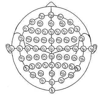
one second. The indices of the 64 electrodes are 153

"FP1", "FP2", "F7", "F8", "AF1", "AF2", "FZ", 154

"F4", "F3", "FC6", "FC5", "FC2", "FC1", "T8", 155

"T7", "CZ", "C3", "C4", "CP5", "CP6", "CP1", 156

"CP2", "P3", "P4", "PZ", "P8", "P7", "PO2", 157

"PO1", "O2", "O1", "X", "AF7", "AF8", "F5", "F6", 158

"FT7", "FT8", "FPZ", "FC4", "FC3", "C6", "C5", 159

"F2", "F1", "TP8", "TP7", "AFZ", "CP3", "CP4", 160

"P5", "P6", "C1", "C2", "PO7", "PO8", "FCZ", 161

"POZ", "OZ", "P2", "P1", "CPZ", "nd" and "Y". 162

The electrodes, "X" and "Y", are EOG signals; and 163

"nd" is the reference electrode. The locations of the 164

EEG electrodes used for data acquisition are shown 165

in Fig. 1. In this paper, the data from 166

SMNI_CMI_TRAIN.tar.gz are used as the training 167

data, and those from SMNI_CMI_TEST.tar.gz are 168

used as the testing data, respectively. 169

[image:2.612.352.513.507.674.2]

170

(3)

3.

METHODOLOGY

172

The workflow of the three proposed data selection 173

methods is shown in Fig. 2. 174

175

[image:3.612.49.274.123.306.2]

176 177 178 179 180 181 182 183 184 185

Fig. 2 The workflow of the proposed methods. 186

Data selection aims at using optimal subsets of 187

variables, while retaining as much useful 188

information as possible. The implementation 189

details are described below. 190

 HVG 191

A HVG is a mapping between time series and 192

complex network [27] according to a specific 193

geometric criterion to make use of methods of 194

complex network theory for characterizing time 195

series. Each datum in the time series corresponds 196

to a node in the graph, such that two nodes are 197

connected if their corresponding data heights are 198

larger than all the data heights between them [28]. 199

Its degree distribution is a good discriminator 200

between randomness and chaos. Let X = (

x

_i ∈ 201

R≥0: i = 1, 2, . . . , n) be an ordered set (or, 202

equivalently, a sequence) of non-negative real 203

numbers. The HVG of X is graph G = (X, E), 204

where X is a set of elements called nodes and E is 205

a set of unordered pairs of nodes called edges. Its 206

definition is shown in equation (1): 207

k i k j

1, (

)

(

)

0,

ij

x

e

otherwise











 





(1)

208

where every k(i, j). In graph theory, the degree 209

of a node (or vertex) of a graph is the number of 210

edges connecting to the node, with loops counted 211

twice [29]. The degree of a vertex is denoted as 212

deg(

x

_i). The degree sequence (DS) is the sequence 213

of the degree of a graph. The node degree and its 214

sequence can be used to describe the characteristics 215

of the graph. 216

In this paper, the time series of EEGs are mapped 217

into graphs (G (X, E)). Each EEG sample is 218

mapped to a HVG, and each HVG has a GE value. 219

There are 1200 samples to be analyzed for each 220

electrode from 10 different trails. Totally 76800 221

features are extracted for 64 electrodes. All GE 222

features are evaluated with groups of alcoholics or 223

non-alcoholics. To illustrate the data 224

transformation process, let us take the dataset 225

co2a0000368 from electrode FP1 in the 226

forementioned database for an example. Given X= 227

{5.015, 5.503, 4.039, 2.085, 0.132, 0.132, 0.621, 228

0.621, 0.132, -0.356, -0.844, -0.356}, we can get 229

the degree sequence DS= {1, 2, 2, 3, 2, 2, 3, 2, 2, 3, 230

2, 2} by the following implementation: 231

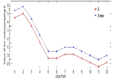
(a). Transform X into Xnew, making every element 232

be a non-negative real number by adding the 233

absolute value of the smallest value which is 234

negative. For example, 235

X= {5.015, 5.503, 4.039, 2.085, 0.132, 0.132, 236

0.621, 0.621, 0.132, -0.356, -0.844, -0.356} 237

should be transformed as 238

Xnew = {5.859, 6.347, 4.883, 2.929, 0.976, 0.976, 239

1.465, 1.465, 0.976, 0.488, 0, 0.488}, which is 240

demonstrated in Fig. 3. 241

242

Fig. 3 Nonnegative transform of X. 243

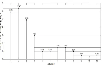
(b). Horizontal visibility check is used to calculate 244

the degree of each node, which is shown in Fig. 4. 245

Two nodes i and j in the graph are connected if one 246

can draw a horizontal line in the time series joining 247

i

x

and

x

_jthat does not intersect any intermediate 248

data height. 249

EEGs

Mathematic Combinations

Kstar

Results PCA-GE Data Selection

Classification KNN GE Difference Based

[image:3.612.343.524.407.536.2]

(4)

[image:4.612.331.541.72.213.2]

250

Fig. 4 The degree of each node from HVGs. 251

(c). Degree sequence. For arbitrary datum in the 252

time series, we calculate the visibility with all the 253

other corresponding nodes and record the number 254

of edges connecting to it as the degree of the node. 255

In the above example, the degree sequence is as 256

follows: 257

DS= {1, 2, 2, 3, 2, 2, 3, 2, 2, 3, 2, 2}. 258

 GE 259

The GE is the entropy of the frequency distribution 260

of the node connections in an undirected and 261

unweighted HVG. It is a function from information 262

theory on a graph G, with a probability distribution 263

( )

p k

on its node set. It was introduced by Janos 264

Korner in [30]. Shannon entropy [31] is used in 265

this paper, which is shown in equation (2): 266

1

( ) log( ( ))

n

k

h

p k



 



(2) 267

where

entropy

is the degree distribution of graph 268

G. The degree distribution p k( ) of a network is 269

defined to be the fraction of nodes in the network 270

with degreek . Thus if there are

n

nodes in total in 271

a network and

k

n of them have degree

k

, we have 272

equation (3) below: 273

k

( )

/

p k



n

(3) 274

In the above case,

p k

( )

of DS is (0, 1/12, 8/12, 275

3/12). The GE is 0.824 when it takes the logarithm 276

base two. The Mean GE plot from 64 electrodes is 277

shown in Fig. 5. From Fig. 5, it is clear that the 278

differences between the alcoholics and the control 279

subjects are indeed different from channel to 280

channel. That is the reason why optimal subsets of 281

channel selection are possible. In this paper, the 282

principal component analysis, the GE difference 283

and the mathematic combinations based on GE 284

channel selection are proposed. The details of the 285

proposed methods are demonstrated below. 286

[image:4.612.94.264.75.183.2]

287

Fig. 5 Mean GE from 64 electrode signals. 288

3.1 The PCA Based on GE from HVG (PCA-GE) 289

Invented by Pearson [32] in 1901, the PCA was 290

widely used in mechanics and independently 291

developed (and named) by Harold Hotelling later 292

in the 1930s [33]. Nowadays, it is used as a tool in 293

exploratory data analysis and for making predictive 294

models. The faithful transformation T = XW maps 295

a data vector X from an original space to a new 296

space of 𝑝variables which are uncorrelated over 297

the dataset. However, not all the principal 298

components are kept. Keeping only the first L 299

principal components, it gives the truncated 300

transformation as shown in equation (4): 301

L L

T = XW

(4)

302

where matrix

L

T now has

n

rows but only

L

303

columns. By reconstruction, all the transformed 304

data matrices reserve only

L

columns out of the 305

original data. Such dimensionality reduction can be 306

a very useful step for visualizing and processing 307

high-dimensional data while keeping as much 308

useful information as possible. In order to keep the 309

same size of input data for the further classification 310

process, here, the corresponding number of the 311

principal components which are the same as that of 312

channels has been chosen. Therefore, the 313

dimensionalities of all the samples are the same. 314

The PCA is implemented in Matlab2013b. The 315

distribution percentage of the total power is shown 316

(5)

[image:5.612.61.279.71.219.2]

318

Fig. 6 The corresponding power percentages of different 319

numbers of the principal components from the full size of data. 320

The PCA-GE technique is applied to extracted 321

representative data transformed from the dataset 322

without specific channel selection investigation. 323

For the alcoholic database, there are 64 electrodes 324

of signals per trial. The inconvenient data 325

preparation and complicated calculations are still 326

challenging for an online analysis and 327

classification system. In the following section, how 328

to gain an optimal subset of specific channels is 329

discussed. 330

3.2 The GE Difference Based Channel Selection 331

From Fig. 5, it is clear that the mean GE differs 332

from electrode to electrode between alcoholic 333

subjects and non-alcoholic ones. Therefore, the 334

channel selection based on the GE difference is 335

proposed. Firstly, the electrodes should be ordered 336

degressively according to the mean GE gap values. 337

They are C1, C2, PO8, PO7, C3, FC2, FCZ, CP2, 338

CPZ, PZ, FZ, CP5, F1, P2, C4, FC1, F2, P4, CP1, 339

P1, CP6, CZ, CP4, AFZ, FC5, AF2, AF1, F8, P3, 340

TP7, T7, POZ, F3, FPZ, FT7, FP1, PO2, AF8, OZ, 341

X, F4, CP3, P6, FC3, PO1, FC4, FT8, O2, Y, F6, 342

P7, P5, nd, C6, C5, TP8, AF7, F7, F5, FC6, T8, P8, 343

FP2, and O1. For comparison reasons, the 344

corresponding specific numbers of channels are 345

selected to generate the optimal subsets for 346

classification. For example, C1 is selected to gain 347

the one-channel subset because the mean GE gap is 348

the largest among all the channels. Similarly, C1 349

and C2 are chosen to gain the two-channel subset, 350

and so on. After that, all the selected data are 351

forwarded to three different classifiers for 352

classification separately. The performance of the 353

proposed channel selection method is demonstrated 354

in the experimental results section. 355

3.3 The Mathematic Combinations Channel 356

Selection 357

In mathematics, a combination is a way of 358

selecting members from a group, and the order of 359

members does not matter. In smaller cases, it is 360

possible to count the number of combinations. 361

More formally, a k-combination of a set S is a 362

subset of k distinct elements of S. If the set has n 363

elements, the number of k-combination is equal to 364

the binomial coefficient. 365

366



 







1 ... 1

1 ...1

k n

n n n k

C

k k

  



 (5) 367

368

which can be written using factorials as ! !( )!

n k nk

if 369

k



n

, and is zero when

k



n

. The set of all k-370

combination of a set S is sometimes denoted by 371

k n

C . 372

Here, mathematic combinations can also be used to 373

select channels from the original 64 electrodes. The 374

proposed method ignores the importance of the 375

individual channels and treats them equally. The 376

main idea of this method is to introduce a simple 377

computer-assisted-mathematic-method for medical 378

signals analysis. It seems inefficient to do random 379

mathematic combinations. However, it can easily 380

find out the optimal subsets in a dataset by 381

computers through k n

C runs. In this paper, the 382

average classification accuracy of the ten-time 383

trials with specific numbers of channels chosen by 384

mathematic combinations is demonstrated in the 385

experimental results section for comparison. 386

During the classification process in this paper, the 387

extracted data from the previous data selection 388

stage are classified by three different classifiers, 389

namely: the J48 decision tree, the K-nearest 390

neighbor (KNN) and the Kstar. The details of the 391

classifiers are introduced in this section. 392

 J48 Decision Tree 393

The J48 decision tree (Weka implementation of 394

C4.5) was published by Ross Quinlan in 1993 [34]. 395

It is a classic method to represent information from 396

a machine learning algorithm and offers a fast and 397

powerful means to express structures in data [35]. 398

In this paper, the J48 algorithm provided by Weka 399

is used. Weka is an open-source Java application 400

produced by the University of Waikato in New 401

Zealand. This software offers an interface through 402

which many algorithms can be utilized on pre-403

formatted datasets. Using this interface, several test 404

0.4 0.5 0.6 0.7 0.8 0.9 1

1 6 11 16 21 26 31 36 41 46 51 56 61

P

o

w

er

P

er

ce

n

ta

g

e

(6)

domains are experimented to gain an insight into 405

the effectiveness of the above three different data 406

selection methods. 407

 K-nearest neighbor (KNN) 408

The KNN algorithm is also selected to conduct the 409

binary classification. The KNN algorithm is a 410

statistical supervised classification which is widely 411

used in traditional pattern recognition techniques 412

[36]. The idea is that given a set of data

t

, the 413

algorithm obtains the K nearest neighbors from 414

the training set based on the distance between

t

415

and the training set. The most dominating class 416

amongst these K neighbors is assigned as class

t

. 417

In this study, the KNN algorithm is implemented 418

as IBK package in Weka 3.7.11. 419

 Kstar 420

The Kstar algorithm is used to evaluate the 421

efficiency of the proposed data selection methods. 422

It can be defined as a method of clustering analysis 423

which aims at partitioning

n

observations into

k

424

clusters in which each observation belongs to a 425

cluster with the nearest mean. The algorithm 426

provides a consistent approach to handle real 427

valued attributes, symbolic attributes and missing 428

values. It uses entropy as a distance measure. In 429

this study, the Kstar algorithm is also implemented 430

in Weka 3.7.11. 431

4.

EXPERIMENTAL RESULTS

432

 Experimental Environment 433

GE is extracted by R x64 3.1.0 and the 434

implementation of the PCA is done by 435

Matlab2013b. The classification is performed using 436

the J48 decision tree, the KNN and the Kstar in 437

Weka 3.7.10. All experiments are performed on a 438

3.40GHz Intel(R) Core(TM) i7-3770 CPU 439

processor PC, with 8.00G RAM and 64-bit 440

Operation System. The operation system of the PC 441

is Microsoft Windows 7. 442

 Data Set Selection 443

The experimental EEG datasets consist of two 444

classes (denoted as alcoholic (a) and control (c)). 445

There are 600 samples in

446

SMNI_CMI_TRAIN.tar.gz and 600 samples in 447

SMNI_CMI_TEST.tar.gz from 64 different 448

channels, respectively. In this paper, GE is used to 449

extract features based on HVGs and then the PCA, 450

GE differential based selection or mathematic 451

combinations selection are implemented in 452

choosing the subset of the EEG signals. Each 453

channel data in one second from one sample is 454

mapped to a HVG, and each HVG is extracted as 455

one GE value. Therefore, 76,800 GE features are 456

extracted from the 1200 samples, with each sample 457

having 64 channels. That is to say, both the 458

training data and the testing data are transferred 459

into a [600*64] matrix. 460

Then different subsets of both the training data and 461

the testing data used during the experiments are 462

determined as: (1). Set 1 (1/64 of data), (2). Set 2 463

(2/64 of data), (3). Set 3 (19/64 of data), and (4). 464

Set 4 (64/64 of data). The reason why adopt the 465

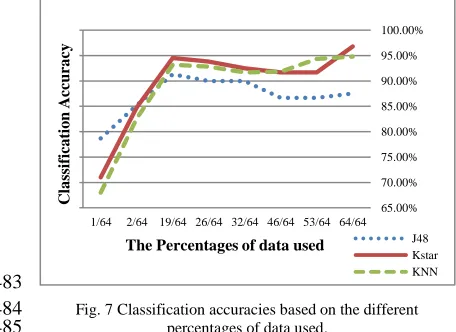
above mentioned sets is illustrated as follows: The 466

classification results based on different percentages 467

of the whole data, which is 1/64, 2/64, 19/64, 26/64, 468

32/64, 39/64, 46/64, 53/64, 64/64, using the J48 469

decision tree, the KNN and the Kstar are displayed 470

in Fig. 7. The classification accuracy increases 471

dramatically when increasing the amount of data 472

used between 1/64 and 19/64. But the accuracy 473

decreases slightly after that and rises again after 474

using 53/64 of the whole data. For online EEG 475

analysis and classification system design, both 476

classification accuracy and the computation time 477

are critical. The redundancy and noise often cause 478

the decrease of the classification efficiency. 479

Therefore, it is significant to select the informative 480

data and eliminate the redundant and misleading 481

data to reduce the computation time. 482

[image:6.612.313.541.427.593.2]

483

Fig. 7 Classification accuracies based on the different 484

percentages of data used. 485

Data selection is expected to preserve as much 486

information as those in the whole database. This 487

paper proposes three data selection methods: (1). 488

the PCA-GE, (2). the GE difference based channel 489

selection, and (3). the mathematic combinations 490

channel selection. In PCA-GE, the four groups of 491

experiments with their power percentages are 492

shown in Table 1. The distributions of the data sets 493

65.00% 70.00% 75.00% 80.00% 85.00% 90.00% 95.00% 100.00%

1/64 2/64 19/64 26/64 32/64 46/64 53/64 64/64

C

la

ssi

fi

ca

ti

o

n

A

cc

u

ra

cy

The Percentages of data used J48

Kstar KNN

(7)

and the PCA selected data are summarized in Table 494

2. 495

Table 1 496

The corresponding power percentages of different numbers of 497

principal components from original data. 498

Table 2 499

The distribution of sample sets and the PCA extracted features. 500

 Performance Comparisons 501

The performances of the PCA-GE method with the 502

experimental EEG datasets using the three different 503

classifiers are evaluated with the aspect of the 504

classification accuracy as shown in Table 3 and the 505

computation time in Table 4. From Tables 3 and 506

Table 4, it is apparent that using 19 out of 64 507

original data can achieve as high as 94.5% 508

accuracy by costing only 29.52% of the 509

computation time, compared to the 96.8% accuracy 510

by using the whole data through the Kstar classifier. 511

Besides, it is interesting to see the improvement of 512

the accuracy from 87.5% to 91.3% by using 19/64 513

data through the J48 decision tree classifier for the 514

PCA-GE data selection method. It is probably due 515

to the filtering of the noise, so that the remaining 516

data are more representative but with much smaller 517

amount. To evaluate the wide applicability of the 518

selected data, three different classifiers are adopted 519

and the one having the highest classification 520

accuracy among the three classifiers is denoted as 521

Bold in the following tables (e.g., Tables 3, 5 and 522

6). 523

Table 3 524

The classification accuracy of the proposed PCA-GE method. 525

Table 4 526

The computation time of the proposed PCA-GE method. 527

Apparently, less data means less computation time. 528

The computation times of all the three proposed 529

methods are reduced significantly when the 530

number of data used decreases as shown in Table 4. 531

In the meantime, the performances of the selected 532

channels subsets based on the mean GE gap values 533

are presented by Table 5 in terms of the 534

classification accuracy. The one-channel signal is 535

from electrode C1. The two-channel data are from 536

electrodes C1 and C2. The 19 channels data are 537

from electrodes C1, C2, PO8, PO7, C3, FC2, FCZ, 538

CP2, CPZ, PZ, FZ, CP5, F1, P2, C4, FC1, F2, P4, 539

CP1; and the 64 channels signals are all the 540

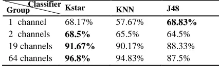
recorded signals from the HVG GEs, respectively. 541

According to our experiment, the proposed GE 542

difference based channel selection method achieves 543

as high as 91.67% classification accuracy by using 544

only 19 out of 64 channels of data for the Kstar 545

classifier. Therefore, it can significantly enhance 546

the efficiency of the EEG data collection. Instead 547

of using all the 64 electrodes placed on the scalp of 548

the subjects, 19 electrodes are enough to gain 549

[image:7.612.332.545.453.518.2]

satisfactory classification results. 550

Table 5 551

The classification accuracy of the GE difference based channel 552

selection. 553

The performances of the selected channels subsets 554

from mathematic combinations are presented by 555

Table 6 in terms of the classification accuracy. 556

Compared to the data selection based on PCA-GE 557

or GE difference, this method neglects the possible 558

different impacts of the individual channels. The 559

method yields an 83.83% classification accuracy 560

when the channel number is 19 through the KNN 561

classifier. 562

Table 6 563

The classification accuracy of the mathematic combinations 564

based channel selection. 565

Set ID No. of Principal Components Power Percentage Set 1 1 0.479

Set 2 2 0.637

Set 3 19 0.935

Set 4 64 1

Set ID Training Set Testing Set Total

Set 1 [600 x 1] [600 x 1] [1200 x 1]

Set 2 [600 x 2] [600 x 2] [1200 x 2]

Set 3 [600 x 19] [600 x 19] [1200 x 19]

Set 4 [600 x 64] [600 x 64] [1200 x 64]

Kstar KNN J48

1 component 71.0% 68.0% 78.7%

2 components 84.8% 82.5% 85.2%

19 components 94.5% 93.2% 91.3%

64 components 96.8% 94.8% 87.5%

Kstar KNN J48

1 component 0.63s 0.01s 0.01s

2 components 1.28s 0.01s 0.02s 19 components 11.51s 0.06s 0.03s 64 components 38.99s 0.10s 0.04s

Kstar _KNN J48

1 channel 68.17% 57.67% 68.83%

2 channels 68.5% 65.5% 64.5%

19 channels 91.67% 90.17% 88.33%

64 channels 96.8% 94.83% 87.5%

Group Classifier

Group

Group Classifier

(8)

In summary, all the proposed methods have been 566

proved to yield an acceptable classification 567

accuracy using significantly reduced amount of 568

data. The results validate the efficiency of the 569

proposed methods in the EEG data reduction. 570

Using as less as possible data to gain high 571

classification performances could significantly 572

reduce the processing time as well as the data 573

collection hardware requirements. 574

5.

DISCUSSION

575

According to experimental results, the proposed 576

PCA-GE algorithm can achieve the comparable 577

accuracy 94.5% by costing only 29.52% of the 578

computation time and using 19 out of 64 original 579

data, compared to the 96.8% accuracy by using the 580

whole 64 channels of the data through the Kstar 581

classifier. Similarly, the proposed GE difference 582

based channel selection method also gets 91.67% 583

classification accuracy by using only 19 out of 64 584

channels of data for the Kstar classifier. They are 585

of high efficiency in terms of both the 586

classification accuracy and the computation time. It 587

is demonstrated that the proposed methods can 588

gain relatively high classification accuracies with a 589

significantly reduced running time during the EEG 590

analysis and classification process. Data selection 591

opens the possibility of using much less 592

representative data to gain satisfactory analysis and 593

classification results 594

6.

CONCLUSSION

595

For multi-channel real EEG signals, using optimal 596

data subsets instead of all the original data and 597

achieving relatively satisfactory classification 598

accuracies with much less computation time are 599

important for EEG analysis and classification. How 600

to get the optimal subsets from the original data is 601

crucial to the following classification performance. 602

In this paper, firstly the GE features from HVGs of 603

the EEG data from alcoholics are calculated. Based 604

on the GE features, the proposed data selection 605

methods are the PCA-GE, the GE difference based 606

channel selection and the mathematic combinations 607

channel selection. It is apparent that less running 608

time is needed by the analysis and classification 609

system if less data are used. Instead of using 610

original data, we extracted features using GE based 611

on HVG. The PCA is successfully used in data 612

selection. Meantime, channel selections based on 613

GE difference and mathematic combinations are 614

proposed for the purpose of comparisons. All of 615

them can gain high classification accuracy as well 616

as decrease the computation time, which is 617

important for the design of the online EEG signals 618

analysis and classification system. Data selection 619

using PCA-GE algorithm was found to be more 620

efficient and beneficial. 621

REFERENCES 622

[1] Haas LF (2003) Hans Berger (1873–1941), Richard Caton

623

(1842–1926), and electroencephalography. Journal of

624

Neurology, Neurosurgery & Psychiatry 74 (1):9-9

625

[2] Lehnertz K, Elger CE (1998) Can Epileptic Seizures be

626

Predicted? Evidence from Nonlinear Time Series Analysis of

627

Brain Electrical Activity. Physical Review Letters 80

628

(22):5019-5022

629

[3] Martinerie J, Adam C, Quyen MLV, Baulac M, Clemenceau

630

S, Renault B, Varela FJ (1998) Epileptic seizures can be

631

anticipated by non-linear analysis. Nat Med 4

(10):1173-632

1176

633

[4] Siuly S, Kabir E, Wang H, Zhang Y (2015) Exploring

634

Sampling in the Detection of Multicategory EEG Signals.

635

Computational and Mathematical Methods in Medicine

636

2015:576437. doi:10.1155/2015/576437

637

[5] Siuly, Li Y, Wen P (2011) EEG signal classification based on

638

simple random sampling technique with least square support

639

vector machine. International Journal of Biomedical

640

Engineering and Technology 7 (4):390-409.

641

doi:10.1504/IJBET.2011.044417

642

[6] Zhu G, Li Y, Wen P (2011) Evaluating functional

643

connectivity in alcoholics based on maximal weight

644

matching. Journal of Advanced Computational Intelligence

645

and Intelligent Informatics 15 (9):1221-1227

646

[7] Wackermann J (1995) Beyond mapping: estimating

647

complexity of multichannel EEG recordings. Acta

648

neurobiologiae experimentalis 56 (1):197-208

649

[8] Zhu G, Li Y, Wen PP (2012) An efficient visibility graph

650

similarity algorithm and its application on sleep stages

651

classification. In: Brain Informatics. Springer, pp 185-195

652

[9] Stam C, Lelj EHvd, Keunen R, Tavy D (1999) Nonlinear

653

EEG changes in postanoxic encephalopathy. Theory in

654

Biosciences-Theorie in den Biowissenschaften 118

(3-655

4):209-218

656

[10] Stam CJ, Van Woerkom T, Keunen R (1997) Non-linear

657

analysis of the electroencephalogram in Creutzfeldt-Jakob

658

disease. Biological cybernetics 77 (4):247-256

659

[11] Nguyen-Ky T, Wen P, Li Y, Malan M (2012) Measuring the

660

hypnotic depth of anaesthesia based on the EEG signal using

661

combined wavelet transform, eigenvector and normalisation

662

techniques. Computers in biology and medicine 42

(6):680-663

691

664

[12] Li T, Wen P, Jayamaha S (2014) Anaesthetic EEG signal

665

denoise using improved nonlocal mean methods.

666

Australasian Physical & Engineering Sciences in Medicine

667

37 (2):431-437

668

[13] Misulis KE, Spehlmann R (1994) Spehlmann's evoked

669

potential primer: visual, auditory, and somatosensory evoked

670

potentials in clinical diagnosis. Butterworth-Heinemann

671

Medical,

672

[14] Oscar-Berman M, Marinković K (2007) Alcohol: effects on

673

neurobehavioral functions and the brain. Neuropsychology

674

review 17 (3):239-257

675

[15] Richman JS, Moorman JR (2000) Physiological time-series

676

analysis using approximate entropy and sample entropy.

677

American Journal of Physiology-Heart and Circulatory

678

Physiology 278 (6):H2039-H2049

679

Kstar KNN J48

1 channel 58% 54.18% 58%

2 channels 58.33% 59.5% 61%

19 channels 81.33% 83.83% 78.5%

64 channels 96.8% 94.83% 87.5%

(9)

[16] Di W, Zhihua C, Ruifang F, Guangyu L, Tian L Notice of

680

Retraction Study on human brain after consuming alcohol

681

based on EEG signal. In: Computer Science and Information

682

Technology (ICCSIT), 2010 3rd IEEE International

683

Conference on, 2010. IEEE, pp 406-409

684

[17] Sun Y, Ye N, Xu X EEG analysis of alcoholics and controls

685

based on feature extraction. In: Signal Processing, 2006 8th

686

International Conference on, 2006. IEEE,

687

[18] Subasi A (2007) EEG signal classification using wavelet

688

feature extraction and a mixture of expert model. Expert

689

Systems with Applications 32 (4):1084-1093

690

[19] Güler I, Übeyli ED (2005) Adaptive neuro-fuzzy inference

691

system for classification of EEG signals using wavelet

692

coefficients. Journal of neuroscience methods 148

(2):113-693

121

694

[20] Tsuji T, Bu N, Fukuda O, Kaneko M (2003) A recurrent

log-695

linearized Gaussian mixture network. Neural Networks,

696

IEEE Transactions on 14 (2):304-316

697

[21] Vasicek O (1976) A test for normality based on sample

698

entropy. Journal of the Royal Statistical Society Series B

699

(Methodological):54-59

700

[22] Polat K, Güneş S (2007) Classification of epileptiform EEG

701

using a hybrid system based on decision tree classifier and

702

fast Fourier transform. Applied Mathematics and

703

Computation 187 (2):1017-1026

704

[23] Chandaka S, Chatterjee A, Munshi S (2009)

Cross-705

correlation aided support vector machine classifier for

706

classification of EEG signals. Expert Systems with

707

Applications 36 (2):1329-1336

708

[24] Zhu G, Li Y, Wen PP, Wang S (2014) Analysis of alcoholic

709

EEG signals based on horizontal visibility graph entropy.

710

Brain Informatics:1-7

711

[25] Tomida, Naoki, et al. "Active Data Selection for Motor

712

Imagery EEG Classification." Biomedical Engineering, IEEE

713

Transactions on 62.2 (2015): 458-467.

714

[26] Bache K, Lichman M (2013) UCI machine learning

715

repository. URL http://archive. ics. uci. edu/ml, vol 901.

716

[27] Gutin G, Mansour T, Severini S (2011) A characterization of

717

horizontal visibility graphs and combinatorics on words.

718

Physica A: Statistical Mechanics and its Applications 390

719

(12):2421-2428

720

[28] Luque B, Lacasa L, Ballesteros F, Luque J (2009) Horizontal

721

visibility graphs: Exact results for random time series.

722

Physical Review E 80 (4):046103

723

[29] Diestel R (2005) Graph Theory (3rd ed'n).

724

[30] Körner J Coding of an information source having ambiguous

725

alphabet and the entropy of graphs. In: 6th Prague conference

726

on information theory, 1973. pp 411-425

727

[31] Shannon CE (2001) A mathematical theory of

728

communication. ACM SIGMOBILE Mobile Computing and

729

Communications Review 5 (1):3-55

730

[32] Person K (1901) On lines and planes of closest fit to systems

731

of points in space. philosophical magazine 2 (6):559-572

732

[33] Hotelling H (1933) Analysis of a complex of statistical

733

variables into principal components. Journal of educational

734

psychology 24 (6):417

735

[34] Salzberg SL (1994) C4. 5: Programs for machine learning by

736

j. ross quinlan. morgan kaufmann publishers, inc., 1993.

737

Machine Learning 16 (3):235-240

738

[35] Sehgal L, Mohan N, Sandhu PS Quality prediction of

739

function based software using decision tree approach. In:

740

International Conference on Computer Engineering and

741

Multimedia Technologies (ICCEMT), 2012. pp 43-47

742

[36] Duda RO, Hart PE (1973) Pattern classification and scene

743

analysis. vol 3. Wiley New York,

RL http://archive.