A&A 584, A84 (2015)
DOI:10.1051/0004-6361/201525993 c
ESO 2015
Astronomy
&
Astrophysics
A maximum entropy approach to detect close-in giant planets
around active stars
P. Petit
1,2, J.-F. Donati
1,2, E. Hébrard
1,2, J. Morin
3, C. P. Folsom
4,5, T. Böhm
1,2, I. Boisse
6, S. Borgniet
4,5,
J. Bouvier
4,5, X. Delfosse
4,5, G. Hussain
1,2,7, S. V. Je
ff
ers
8, S. C. Marsden
9, and J. R. Barnes
101 Université de Toulouse, UPS-OMP, Institut de Recherche en Astrophysique et Planétologie, 31000 Toulouse, France e-mail:[email protected]
2 CNRS, Institut de Recherche en Astrophysique et Planétologie, 14 Avenue Édouard Belin, 31400 Toulouse, France 3 LUPM-UMR 5299, CNRS & Université Montpellier II, Place Eugène Bataillon, 34095 Montpellier Cedex 05, France 4 Univ. Grenoble Alpes, IPAG, 38000 Grenoble, France
5 CNRS, IPAG, 38000 Grenoble, France
6 Université Aix-Marseille/CNRS-INSU, LAM/UMR 7326, 13388 Marseille, France
7 European Southern Observatory, Karl-Schwarzschild-Str. 2, 85748 Garching bei München, Germany
8 Institut für Astrophysik, Georg-August-Universität Göttingen, Friedrich-Hund-Platz 1, 37077 Göttingen, Germany 9 Computational Engineering and Science Research Centre, University of Southern Queensland, 4350 Toowoomba, Australia 10 Centre for Astrophysics Research, University of Hertfordshire, College Lane, Hatfield, Herts AL10 9AB, UK
Received 28 February 2015/Accepted 25 August 2015
ABSTRACT
Context.The high spot coverage of young active stars is responsible for distortions of spectral lines that hamper the detection of close-in planets through radial velocity methods.
Aims.We aim to progress towards more efficient exoplanet detection around active stars by optimizing the use of Doppler imaging in radial velocity measurements.
Methods.We propose a simple method to simultaneously extract a brightness map and a set of orbital parameters through a tomo-graphic inversion technique derived from classical Doppler mapping. Based on the maximum entropy principle, the underlying idea is to determine the set of orbital parameters that minimizes the information content of the resulting Doppler map. We carry out a set of numerical simulations to perform a preliminary assessment of the robustness of our method, using an actual Doppler map of the very active star HR 1099 to produce a realistic synthetic data set for various sets of orbital parameters of a single planet in a circular orbit.
Results.Using a simulated time series of 50 line profiles affected by a peak-to-peak activity jitter of 2.5 km s−1, in most cases we are able to recover the radial velocity amplitude, orbital phase, and orbital period of an artificial planet down to a radial velocity semi-amplitude of the order of the radial velocity scatter due to the photon noise alone (about 50 m s−1in our case). One noticeable exception occurs when the planetary orbit is close to co-rotation, in which case significant biases are observed in the reconstructed radial velocity amplitude, while the orbital period and phase remain robustly recovered.
Conclusions.The present method constitutes a very simple way to extract orbital parameters from heavily distorted line profiles of active stars, when more classical radial velocity detection methods generally fail. It is easily adaptable to most existing Doppler imaging codes, paving the way towards a systematic search for close-in planets orbiting young, rapidly-rotating stars.
Key words.planets and satellites: detection – stars: imaging – stars: rotation – stars: activity – planetary systems
1. Introduction
The numerous detections of exoplanets reported in the last two decades highlight the relatively small population of planets dis-covered around young stars. These lack of detections, because of the limitations of existing techniques, are especially obvious in studies based on radial velocity (RV) analysis, with a very low number of planets reported around stars younger than about 300 myr (Setiawan et al. 2007; Borgniet et al. 2014). The en-hanced activity of young Sun-like stars, linked to their fast rota-tion rate (Gallet & Bouvier 2013), is the main barrier to RV mea-surements (Saar & Donahue 1997;Queloz et al. 2001). Since the heavy spot coverage of these young objects generates a RV jit-ter that can hide most planetary signatures, filjit-tering the activity noise is a prerequisite to progress towards a more accurate search for planets orbiting young stars. Our main motivation is to bet-ter constrain the formation mechanisms of planetary systems by
comparing the observed prevalence of hot jupiters versus model predictions (Mordasini et al. 2009), as well as to get a more com-prehensive view of the evolution of accretion disks and debris disks in the presence of planets (Ida & Lin 2005).
A number of studies have been dedicated to progress to-wards more efficient filtering of activity jitter in RV curves (e.g. Reiners et al. 2010;Boisse et al. 2012;Dumusque et al. 2014; Jeffers et al. 2014;Hébrard et al. 2014). For fast-rotating stars, Doppler imaging (DI) maps can be used to perform a RV fil-tering taking a complex distribution of active regions over the stellar surface into account (Donati et al. 2014). We propose a different approach, which does not use the two-step method of previous studies in which Doppler mapping is performed prior to the RV analysis. Instead, we implement the recovery of orbital parameters in the DI inversion procedure itself. We therefore do not operate an explicit filtering of the RV curve (we actually do
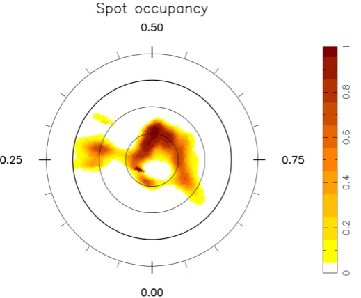
Fig. 1.Spot occupancy on the artificial star, in flattened polar view, from observations of HR 1099 secured in 1998 January. Concentric circles represent, starting from the centre, parallels of latitude+60,+30, 0, and−30◦
. Radial ticks around the star illustrate the rotational phases, with steps of 0.05 rotation cycle, followingDonati et al.(2003b).
not extract any RVs from our data), but simultaneously get a brightness map and a set of orbital parameters in the output of a slightly modified DI model. Our method shares many similari-ties with a technique previously implemented to measure stel-lar rotation and differential rotation (Donati et al. 2000; Petit et al. 2002), which proved to behave very robustly in a num-ber of practical cases (Donati et al. 2003a;Barnes et al. 2005; Petit et al. 2008,2010).
In the rest of the paper, we first present our set of simulated data, detail our maximum entropy approach to extract the orbital elements of an artificial planet, and then present some prelim-inary tests of the method for various sets of orbital parameters. We finally list our conclusions and mention future tests that need to be performed to fully assess the efficiency of this technique.
2. Simulated data
The spotted surface of the artificial star considered here is based on a Doppler map of the very active star HR 1099, reproduced on a sphere divided into a grid of 20 000 rectangular pixels of approximately equal area (Fig.1). This map was initially recon-structed from data collected at the Anglo-Australian Telescope in 1998 January (Donati et al. 2003b) and features a number of large spots distributed from the equator to the observed pole. With a total spot coverage of about six per cent, this specific brightness distribution is a good illustration of the high spot cov-erage of cool, rapidly rotating stars (e.g. Donati et al. 2003b; Marsden et al. 2006,2011;Waite et al. 2015).
We use this spot distribution to produce a set of synthetic cross-correlation profiles, using the set of tools previously em-ployed byPetit et al.(2002). We assume here that the projected rotational velocity (vsini) of the star is equal to 40 km s−1, and that its inclination angle is equal to 38◦(following the values of Donati et al. 2003b). The unspotted surface temperature is set to 5500 K, and the spot temperature is equal to 3500 K. We as-sume a spectral resolving power R = 65 000 (with a Gaussian instrumental profile), and compute line profiles projected on ve-locity bins of 1.8 km s−1for a total of 50 rotational phases evenly
Fig. 2.Simulated line profiles (normalized to the continuum level) gen-erated from the artificial star of Fig.1, in the absence of a planetary companion. Successive profiles are vertically shifted for display clar-ity and the rotational phase of simulated observation is given in the right side of the plot (with the integer part indicating the rotation cycle number).
spread over three consecutive stellar rotation cycles (Fig.2). We finally simulate photon noise by adding a Gaussian noise to the line profiles, resulting in a signal-to-noise ratio (S/N) of 1000 per velocity bin.
The resulting line profiles are consistent with typical obser-vations of rapidly-rotating, solar-type stars, and, in particular, young Suns. The S/N is at a level commonly reached in a num-ber of published DI studies (e.g.Donati et al. 2003b), especially when cross-correlation pseudo-line profiles are modelled instead of individual spectral lines (Donati et al. 1997). In this case,
S/N=1000 in the cross-correlation profile implies a S/N about 30 times lower in the initial spectrum. Gathering 50 rotational phases in a single run and in a time span sufficiently short to pre-vent any significant spot evolution is demanding but not unreal-istic, in particular, for stars with rotation periods of a few days, displaying significant phase evolution within a single observing night. We stress however that the regularity of the phase cov-erage proposed here is unlikely to be reached from the ground because of observation gaps during the daytime. The impact of these daytime observations gaps can be at least partly reduced in the case of multi-site campaigns (e.g.Petit et al. 2004).
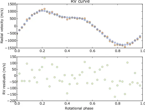
[image:2.595.39.299.74.288.2]Fig. 3.Radial velocity time series extracted from our set of simulated cross-correlation profiles using the first moment method (top panel, orange dots), plotted together with radial velocities produced by the Doppler imaging code (blue dots). This model does not include any or-biting planet.The bottom panelshows the RV residuals.
rms scatter of 66 m s−1 only (this value being a function of the adopted S/N and velocity bin size), so that the standard deviation of RVs is dominated by the simulated spot activity.
We finally alter the line profiles to incorporate RV shifts due to the presence of a close-in planet, assuming that the instru-ment benefits from perfect RV stability. For simplicity, we as-sume here a single planetary companion, following a circular orbit. The orbit and stellar equator share the same plane. The time-dependent RV shift induced by the companion is defined by the ratio of orbital over (stellar) rotation periods (Porb/Prot), its semi-amplitude (K), and its phase delay (φ) compared to stel-lar rotation. We define the phase delay so that it is equal to zero if the first observed stellar rotational phase (also set to zero) is a time of maximal planetary-induced RV shift.
3. Simultaneous maximum entropy inversion of the brightness map and orbital parameters
3.1. Method outline
We use here a maximum entropy approach to simultaneously reconstruct the stellar brightness map and orbital parameters from the set of simulated observations. With this strategy, or-bital parameters are directly included in the DI model, similarly to relevant stellar parameters (e.g. stellar inclination or vsini). Following the very basic principle of maximum entropy image reconstruction, the most likely value for the triplet of orbital pa-rameters is the value that produces a brightness map with the lowest information content, i.e. the reconstructed map featuring the lowest spot coverage.
In practice, we adapt the method successfully implemented byPetit et al.(2002) to recover the surface differential rotation of active stars, by computing a grid of Doppler images spanning a range of values ofK,Porb/Prot, andφ. This method is directly inspired from the “entropy landscape” method of Donati et al. (2000) andWatson & Dhillon(2001), although transposed to a 3D parameter space. We reconstruct the brightness maps using the DI code of Donati & Collier Cameron (1997), which im-plements the two-component model ofCollier Cameron(1992).
This model is based on the assumption that each pixel of the reconstructed stellar surface contains a fraction f of unspotted photosphere and a fraction 1−f of dark spot. From the same sim-ulated data set (i.e. for the same simsim-ulated value ofK,Porb/Prot andφ), we reconstruct a set of 1000 to 3375 Doppler maps, as-suming different values of the (K,Porb/Prot,φ) triplet in the in-version process. We derive from each reconstructed map a value of the fractional spot coverage and therefore obtain a 3D spot-tedness landscape in the (K,Porb/Prot,φ) space (Fig.4). To de-termine the reconstructed value of (K,Porb/Prot,φ), we adjust a 3D paraboloid in the (K,Porb/Prot,φ) space, limiting the fit to a few tens of points around the point of minimal spottedness. By locating the point of minimal information content of the Doppler map, the paraboloid fit gives the most likely output value for (K,
Porb/Prot,φ).
Similar to the method adopted byPetit et al. (2002), error bars shown in Figs.5−7are derived from the paraboloid fit by determining the projection on the three axis of the∆χ2=1 sur-face surrounding theχ2minimum, following the prescription of Press et al.(1992). Since the reconstructed orbital parameters are computed from DI models, their estimate benefits from an effi -cient noise reduction technique (the maximum entropy method), which tends to decrease the uncertainties in their reconstructed values beyond the capabilities of a simpleχ2minimization ap-proach. In this sense, usingχ2values alone to derive statistical uncertainties, as we do here, implies that all error bars discussed in the following sections are likely over-estimated.
We do not perform an explicit filtering of activity jitter in line profiles, as done byDonati et al.(2014). Instead, we obtain the orbital parameters as part of the image reconstruction itself, although the reconstructed line profiles produced by the DI code, in principle, can be used to perform a jitter filtering of observa-tional data to double check the orbital parameters identified with our method (Fig.3). We emphasize that the rough atmospheric model used in the DI code is the same as that used to produce our fake data, so that we implicitly assume here that the DI at-mospheric model is perfect.
3.2. Test case without a planet
The first test of our technique consisted of simulating a star with-out any planet (K,Porb/Prot,φ)=(0, 0, 0) and checking the out-come of the Doppler inversion. The simulated set of line profiles is shown in Fig. 2 and the resulting map (not shown here) is reconstructed with a reducedχ2close to unity (χ2
r =0.97). The initial spot configuration is correctly recovered, with the location and area of the reconstructed spots consistent with the initial spot configurations. Using the set of line profiles produced by the DI code to remove the activity-induced RV fluctuations from our simulated data, we end up with a rms residual jitter of 68 m s−1, which is very slightly larger than the rms scatter induced by the simulated photon noise alone (bottom panel of Fig.3), showing that our simulated observations were adjusted down to the noise level, with no detectable residuals of the activity jitter in the fil-tered RV curve.
1.60 1.65 1.70 1.75 1.80 1.85 Porb / Prot
0.00 0.05 0.10 0.15
Phase
0.000002 0.000008 0.000014 0.000020 0.000026 0.000032 0.000038 0.000044 +5.597e 2
1.60 1.65 1.70 1.75 1.80 1.85
Porb / Prot 0.40
0.45 0.50 0.55
Phase
[image:4.595.311.545.67.639.2]0.000000 0.000004 0.000008 0.000012 0.000016 0.000020 0.000024 0.000028 0.000032 0.000036 +5.596e 2
Fig. 4. Top panel: example 3D entropy (spottedness) landscape, ob-tained from 1000 DI models with different values ofK,Porb/Prot, andφ. The simulated parameter values wereK =0.1 km s−1 P
orb/Prot =1.7 andφ=0.5.Middle and bottom panels: example 2D slices in two or-thogonal planes, extracted from the 3D orbital parameter space. Each slice is obtained from a set of 2500 Doppler images. In all three pan-els, the colour scale shows the fractional spot coverage of the resulting Doppler maps, and the location of minimal spottedness shows the re-constructed set of orbital parameters.
compared to higherKinvalues (see Sect.3.3.1), is a consequence of the correlation between the different parameters of the triplet,
0 50 100 150 200
Input K (m/s) 50
100 150 200
Reconstructed K (m/s)
0 50 100 150 200
Input K (m/s) 1.0
1.2 1.4 1.6 1.8 2.0 2.2 2.4
Reconstructed Porb / Prot
0 50 100 150 200
Input K (m/s) 0.0
0.2 0.4 0.6 0.8 1.0
[image:4.595.54.279.74.630.2]Reconstructed phase
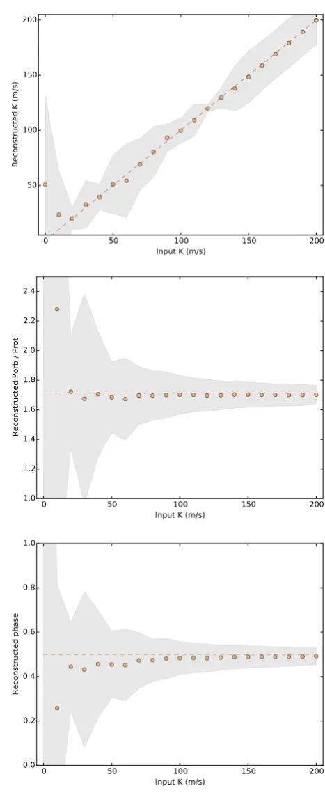
Fig. 5.Simulations for a radial velocity amplitudeK varying from 0 to 200 m s−1. The orbital period is fixed and equal to 1.7 times the rota-tional period, as well asφ, which is set to 0.5. The dashed lines indicates the input values, while circles show the reconstructed parameters. The 1σerror bars derived on individual parameters from the paraboloid fit are plotted as grey areas.
0.6 0.8 1.0 1.2 1.4 1.6 1.8 2.0 Input Porb / Prot
0 50 100 150 200
Reconstructed K (m/s)
0.6 0.8 1.0 1.2 1.4 1.6 1.8 2.0
Input Porb / Prot 0.6
0.8 1.0 1.2 1.4 1.6 1.8 2.0
Reconstructed Porb / Prot
0.6 0.8 1.0 1.2 1.4 1.6 1.8 2.0 Input Porb / Prot
0.0 0.2 0.4 0.6 0.8 1.0
[image:5.595.51.279.70.638.2]Reconstructed phase
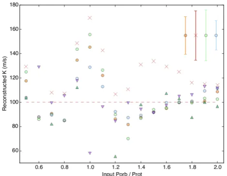
Fig. 6. Same as Fig.5, except for an orbital period varying from 0.5 to 2 times the stellar rotation period. The radial velocity amplitudeKis fixed and equal to 100 m s−1andφ, which is set to 0.5.
3.3. Orbital parameter reconstruction
The next test consisted of running a series of simulations with different input values of (K,Porb/Prot,φ) to test the robustness of the method for different orbital configurations.
0.0 0.2 0.4 0.6 0.8
Input phase 0
50 100 150 200
Reconstructed K (km/s)
0.0 0.2 0.4 0.6 0.8
Input phase 1.4
1.5 1.6 1.7 1.8 1.9 2.0
Reconstructed Porb / Prot
0.0 0.2 0.4 0.6 0.8
Input phase 0.0
0.2 0.4 0.6 0.8
Reconstructed phase
Fig. 7.Same as Fig.5, except for an orbital phase varying from 0 to 0.9. The radial velocity amplitudeKis fixed and equal to 100 m s−1and
Porb/Prot, which is set to 1.7.
3.3.1. Variations ofK
[image:5.595.308.544.72.638.2]20 m s−1 (up to 35 m s−1 atKin = 60 m s−1). For even smaller simulated values ofKin, the reconstructed values display much larger biases towards higher RV amplitudes, with error bars in-creasing very fast whenKinapproaches zero.
The reconstructed values of Porb/Prot are also very close to the input values (to within 2%), as long as the input Kin is larger than 20 m s−1. The error bars onPorb/P
rot progressively increase whileKindecreases, going from 0.05 atKin=200 m s−1 to 0.6 at Kin = 30 m s−1, and remain large whenever Kin < 50 m s−1. The reconstruction biases also become much larger for
Kin<20 m s−1.
The behaviour of the reconstructedφis mostly similar to that ofPorb/Prot, with more systematic biases at low values ofKin.
3.3.2. Variations ofPorb/Prot
We also performed a series of simulations at fixed values of
Kin = 100 m s−1, andφin = 0.5. Here, (Porb/Prot)in was varied from 0.5 to 2 (Fig.6). The reconstructed (Porb/Prot) is always close to its input value, without any systematic bias. The error bar on the recovered value of (Porb/Prot) is steadily increasing to-wards larger values of (Porb/Prot)in, showing that it is preferable to spread the observations over several orbital periods, rather than getting a denser sampling of one single orbital cycle.
The most striking feature in the reconstructedKvalues is a clear bias of up to 50% whenPorb ≈ Prot, although the recon-structed (Porb/Prot) and φ are much less affected by this phe-nomenon. The poor reconstruction obtained for a planet close to co-rotation, already reported byDonati et al.(2014), illustrates that the modified DI code cannot fully distinguish between a spot and a planetary signature as long as the rotational and orbital modulations are not following a different period. As illustrated in Fig.8, adding a different noise pattern to our data (with a same resulting S/N) does not remove this bias. Apart from this zone, biases in the reconstructedKdo not exceed 20%, and get even better at (Porb/Prot)>1.6.
3.3.3. Variations ofφ
The last test consisted of varyingφin, at fixed values ofKinand (Porb/Prot)in(Fig.7). The outcome is an accurate reconstruction of the triplet for all values ofφin, with limited biases for all or-bital parameters, suggesting that theφparameter is the less crit-ical of the triplet in this reconstruction procedure.
4. Impact of uncertainties in reconstruction parameters
[image:6.595.315.550.75.257.2]In our ideal numerical simulations, setting reconstruction param-eters in the DI code is straightforward in that we know the pa-rameters used to generate the artificial star and fake time series of observations exactly. This question is notoriously more diffi -cult with real data, and errors in the parameters adopted in the DI procedure are known to generate biases in the reconstruction of stellar brightness maps (Unruh & Collier Cameron 1995). We carried out a preliminary investigation of the outcome of wrong values of DI input parameters in the reconstructed triplet of or-bital parameters. We based this new series of tests on simulations similar to those discussed in Sect.3.3.2, i.e. where the RV am-plitudeKis fixed and equal to 100 m s−1, as well asφ, which is set to 0.5, whilePorb/Protis varied between 0.5 and 2.0. The re-constructedKvalues obtained in this new series of simulations are shown in Fig.8.
Fig. 8.Same as the top panel of Fig.6, with errors introduced in the re-construction parameters. Orange circles again show the points of Fig.6, obtained withχ2
r =0.97 andi=38
◦
, i.e. our optimal model. Green and pale blue circles are obtained by forcingχ2
r =1.0 and 0.94, respectively, during reconstruction. Violet (resp. green) triangles show the effect of forcingi=33◦
(resp.i=43◦
). Crosses are obtained by adding another noise pattern to our fake data set (using a different seed to generate ran-dom numbers, still resulting inS/N ≈ 1000). Typical error bars are indicated in the top right side of the plot, except for violet and green tri-angles (affected by much larger statistical error bars that would hamper the plot readability).
A first test consisted in varying the final χ2r values of the models. Instead of the default target value of 0.97, which is set to be the highestχ2r value below which the rms of the RV residu-als cannot be reduced further,χ2
r =1.0 and 0.94 are successively adopted (circles in Fig.8). We observe that reconstruction biases inKvalues tend to decrease for decreasingχ2
r values and the as-sociated error bars. However, the observed changes remain lim-ited compared to other effects. In particular, adoptingχ2
r =0.97 again with a different noise pattern in our data (simply obtained with a different seed to generate random numbers, red crosses in Fig.8) roughly leads to the same amplitude of changes in the biases and error bars. Similar conclusions are reached for the reconstruction ofPorb/Protandφ(not shown here). Belowχ2r = 0.94, most of our models did not converge at all.
As a second test, we modified the inclination angle assumed during the inversion process, adoptingi = 33 and 43◦ instead of i = 38◦ (triangles in Fig. 8). While some of these models still provided us with reconstructedKvalues close to the input value, the biases become much larger in a number of cases to the point where several points fall outside of the boundaries of our figure. The obvious inaccuracy in the inclination angle is also highlighted by the best achievableχ2
r , which is more than doubled that of our models assuming an optimal value for the stellar inclination. In practice, these largeχ2
r values suggest that offsets on the inclination angle in the DI input parameters should remain smaller in real cases. Not surprisingly, statistical error bars are also very large, up to ten times wider than those of our optimal model.
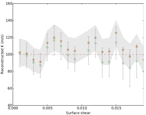
Fig. 9.ReconstructedKvalues obtained with stellar models, including various levels of solar-like surface differential rotation. The dimension-less surface shear is equal to dΩ/Ωeq, whereΩeq is the rotation rate of the equator andΩis the difference of rotation rate between the pole and the equator. Orange dots and their error bars (grey area) correspond to DI models compensating for the differential rotation (Petit et al. 2002). Green dots are obtained with DI models assuming solid-body rotation.
the pole and the equator. We varied the dimensionless parameter γ = dΩ/Ωeqfrom zero (solid-body rotation) to 0.02, assuming (K,Porb/Prot, φ)=(100 m s−1,1.7,0.5). Assuming a star rotating in three days,γ=0.02 roughly corresponds to 80% of the solar shear level. In this case, our artificial data (assumed to be gath-ered over three stellar rotation cycles) are collected over nine consecutive days. Some of our DI models compensate for diff er-ential rotation (Petit et al. 2002, orange dots). Other DI models simply ignore the shear by assuming solid-body rotation (green dots), showing the consequence of obtaining an incorrect esti-mate of the shear, or of using an incorrect type of differential rotation law. Figure 9 shows that the biases and error bars re-main roughly constant for DI models incorporating a diff eren-tial rotation law. Up to γ ≈ 0.012, the situation is mostly the same for models assuming solid-body rotation. However, biases steadily increase past this point whenever the surface shear is ignored. This evolution is coming along with a≈25% increase of theχ2
r, and a significant increase in the statistical error bars. Aboveγ=0.02, the majority of our models based on solid-body rotation do not provide any well-defined spottedness minimum in the 3D entropy landscape, so that no reliable values of orbital parameters could be derived. The two differential rotation pa-rameters can be added to the orbital parameter triplet to perform a simultaneous optimization of all five parameters. In this case, the additional dimensions to be probed would likely require us to adopt an MCMC approach to identify the best model, instead of the time-consuming systematic paving of a very large 5D grid. Inclusion of the stellar inclination andvsiniis possible as well, leading to a 7D space to be explored.
5. Conclusions
In spite of a simulated set of line profiles displaying an activity jitter as high as 2.5 km s−1peak to peak, we are able to robustly recover orbital elements of a fake planet with RV signatures of a few tens of m s−1, i.e. of the order of magnitude of the RV scatter due to the photon noise of our simulations. This is true as long as the planet is not in a co-rotating configuration, in which
case offsets of up to 50% are observed in the reconstruction ofK
(assuming Kin = 100 m s−1), while (Porb/Prot) and φ are kept closer to their input values.
Our preliminary tests support the capabilities of this max-imum entropy method in a systematic search for hot jupiters around extremely active stars, as long as the collected time se-ries is well adapted for DI, i.e. with a dense rotational sam-pling collected over a few rotation periods. However, we need to complement the present set of simulations, with a more com-prehensive set of models to determine the detailed effect of a number of parameters (e.g.vsini, stellar inclination, orbital and rotational phase sampling, surface differential rotation) on the reconstruction of planetary orbits. Varying the inclination will mostly become critical at lowi values (i.e. large K/sin(i) val-ues), since the detectability of low-mass planets will be much reduced in this geometrical configuration. The impact ofvsini
is more complex to address. The present approach makes use of the fact that, at large projected rotational velocities, the spectral signatures of individual spots are bumps restricted to a fraction of the line profile, while the planetary signature affects the line profile as a whole. Lowvsinivalues will make this disentan-gling less easy; the limit of efficiency of the technique is there-fore similar to thevsini limit of accurate DI. In any case this threshold is belowvsini=10 km s−1, sinceDonati et al. 2015, demonstrated that the method is still operative for v819 Tau with vsini=9.5 km s−1. On the other hand, if highervsinivalues im-prove the DI efficiency, at the same time it would reduce the RV accuracy, so that an upper limit in projected rotational velocity should exist as well.
In addition, the optimization of our detection threshold will likely require the DI reconstruction of both cool spots and fac-ulae (Donati et al. 2014). Future tests will also assess the ben-efit of obtaining observations at different epochs to take advan-tage of the changing spot occupancy to improve the accuracy of planet detection and characterization in repeated measurements. The impact of non-rotationally modulated events that a classi-cal DI code is not able to model, such as flares or limited spot lifetime, will also deserve special attention.
We also stress that the tests performed here were limited to a single planet following a circular orbit. More complex configu-rations involving an orbital eccentricity or multiple companions will necessitate probing additional dimensions in a multi-D en-tropy landscape. Using any real data set, the average RV of the star-planet system is another parameter that cannot be ignored in the multi-D landscape (seeDonati et al. 2015).
The present maximum entropy method constitutes a very simple way to extract orbital parameters from heavily distorted line profiles of active stars, paving the way towards a system-atic search for close-in planets around young, rapidly-rotating stars. It is easily adaptable to most existing DI codes, and may be employed to revisit a number of existing data sets initially collected for DI purpose alone. One specificity of this technique is the simultaneous extraction of a DI mapand of orbital ele-ments, in a one-step procedure much simpler than the sequen-tial approach generally proposed in this context. In addition to its simpler approach, the lower amount of data manipulation in-volved here is likely to make the present strategy less prone to information removal.
References
Barnes, J. R., Collier Cameron, A., Donati, J.-F., et al. 2005,MNRAS, 357, L1
Boisse, I., Bonfils, X., & Santos, N. C. 2012,A&A, 545, A109
Borgniet, S., Boisse, I., Lagrange, A.-M., et al. 2014,A&A, 561, A65
Collier Cameron, A. 1992, in Lect. Notes Phys. Surface Inhomogeneities on Late-Type Stars, eds. P. B. Byrne, & D. J. Mullan (Berlin Springer Verlag), 397, 33
Donati, J.-F., & Collier Cameron, A. 1997,MNRAS, 291, 1
Donati, J., Semel, M., Carter, B. D., Rees, D. E., & Collier Cameron, A. 1997,
MNRAS, 291, 658
Donati, J.-F., Mengel, M., Carter, B. D., et al. 2000,MNRAS, 316, 699
Donati, J.-F., Collier Cameron, A., & Petit, P. 2003a,MNRAS, 345, 1187
Donati, J.-F., Collier Cameron, A., Semel, M., et al. 2003b,MNRAS, 345, 1145
Donati, J.-F., Hébrard, E., Hussain, G., et al. 2014,MNRAS, 444, 3220
Donati, J.-F., Hébrard, E., Hussain, G., et al. 2015,MNRAS, 453, 3706
Dumusque, X., Boisse, I., & Santos, N. C. 2014,ApJ, 796, 132
Gallet, F., & Bouvier, J. 2013,A&A, 556, A36
Hébrard, É. M., Donati, J.-F., Delfosse, X., et al. 2014,MNRAS, 443, 2599
Ida, S., & Lin, D. N. C. 2005,ApJ, 626, 1045
Jeffers, S. V., Barnes, J. R., Jones, H. R. A., et al. 2014,MNRAS, 438, 2717
Marsden, S. C., Donati, J.-F., Semel, M., Petit, P., & Carter, B. D. 2006,MNRAS, 370, 468
Marsden, S. C., Jardine, M. M., Ramírez Vélez, J. C., et al. 2011,MNRAS, 413, 1922
Mordasini, C., Alibert, Y., Benz, W., & Naef, D. 2009,A&A, 501, 1161
Petit, P., Donati, J.-F., & Collier Cameron, A. 2002,MNRAS, 334, 374
Petit, P., Donati, J.-F., Wade, G. A., et al. 2004,MNRAS, 348, 1175
Petit, P., Dintrans, B., Solanki, S. K., et al. 2008,MNRAS, 388, 80
Petit, P., Lignières, F., Wade, G. A., et al. 2010,A&A, 523, A41
Press, W. H., Teukolsky, S. A., Vetterling, W. T., & Flannery, B. P. 1992, Numerical recipes in FORTRAN, The art of scientific computing (Cambridge University Press)
Queloz, D., Henry, G. W., Sivan, J. P., et al. 2001,A&A, 379, 279
Reiners, A., Bean, J. L., Huber, K. F., et al. 2010,ApJ, 710, 432
Saar, S. H., & Donahue, R. A. 1997,ApJ, 485, 319
Setiawan, J., Weise, P., Henning, T., et al. 2007,ApJ, 660, L145
Unruh, Y. C., & Collier Cameron, A. 1995,MNRAS, 273, 1
Waite, I. A., Marsden, S. C., Carter, B. D., et al. 2015,MNRAS, 449, 8