Re-analyzing the dynamical stability of the HD 47366 planetary system

Re-analyzing the Dynamical Stability of the HD 47366 Planetary System

J. P. Marshall1 , R. A. Wittenmyer2 , J. Horner2 , J. Clark2 , M. W. Mengel2 , T. C. Hinse3 , M. T. Agnew4, and S. R. Kane5

1

Academia Sinica, Institute of Astronomy and Astrophysics, 11F Astronomy-Mathematics Building, NTU/AS campus, No. 1, Section 4, Roosevelt Rd., Taipei 10617, Taiwan

2

University of Southern Queensland, Centre for Astrophysics, Toowoomba, QLD 4350, Australia

3

Department of Astronomy and Space Science, Chungnam National University, Daejeon 34134, Republic of Korea

4

Centre for Astrophysics and Supercomputing, Swinburne University of Technology, Hawthorn, Victoria 3122, Australia

5

Department of Earth Sciences, University of California, 900 University Avenue, Riverside, CA 92521, USA

Received 2018 July 27; revised 2018 October 26; accepted 2018 October 30; published 2018 December 11

Abstract

Multi-planet systems around evolved stars are of interest to trace the evolution of planetary systems into the post-main-sequence phase. HD 47366, an evolved intermediate-mass star, hosts two giant planets on moderately eccentric orbits. Previous analysis of the planetary system has revealed that it is dynamically unstable on timescales much shorter than the stellar age unless the planets are trapped in mutual 2:1 mean-motion resonance, inconsistent with the orbital solution presented in Sato et al., or are moving on mutually retrograde orbits. Here we examine the orbital stability of the system presented in S16 using the n-body code MERCURY over a broad range of a–e parameter space consistent with the observed radial velocities, assuming they are on co-planar orbits. Our analysis confirms that the system as proposed in S16 is not dynamically stable. We therefore undertake a thorough reanalysis of the available observational data for the HD 47366 system, through the Levenberg–Marquardt technique and confirmed by MCMC Bayesian methodology. Our reanalysis reveals an alternative, lower-eccentricityfit that is vastly preferred over the highly eccentric orbital solution obtained from the nominal best-fit presented in S16. The new, improved dynamical simulation solution reveals the reduced eccentricity of the planetary orbits, shifting the HD 47366 system into the edge of a broad stability region, increasing our confidence that the planets are all that they seem to be. Our rigorous examination of the dynamical stability of HD 47366 stands as a cautionary tale infinding the global best-fit model.

Key words:planetary systems– planets and satellites: dynamical evolution and stability–stars: individual(HD 47366)

Supporting material:animations

1. Introduction

Multi-planet systems are important in revealing the influence of planet–planet interactions on the observed architectures and long-term stability of known planetary systems. Caution is needed, however—it is often the case that the best-fit solution for a given planetary system will place the planets therein on dynamically unfeasible orbits—ones that lead to collisions or ejections of those planets on timescales far, far shorter than the age of the system in which they reside (e.g., Horner et al. 2011, 2012; Wittenmyer et al.2012a). In some cases, such dynamically unstable solutions are likely an indication that the observed behavior of the star is driven by a process other than planetary companions(e.g., Horner et al.2012,2013,2014; Wittenmyer et al.2013). In others, it can be a“red-flag”that points to the need for further observations in order to better constrain the proposed planetary orbits (e.g., Wittenmyer et al.2014,2017a; Horner et al. 2018).

The great majority of planet search programs have focused on

“late-type”main-sequence stars—stars similar to, or less massive than the Sun(e.g., Jenkins et al.2006; Fischer et al.2014; Butler et al.2017). In thefirst two decades of the exoplanet era, when the radial velocity technique ruled supreme as a planet detection method, this was unsurprising. More massive main-sequence stars (O, B, and A)have few spectral lines that can be used to determine radial velocities with the precision required for planet search work. On top of this, such stars are typically both active and rapid rotators—characteristics that greatly hinder the detection of small radial velocity signals. More recently, the

balance has shifted somewhat, with the advent of large-scale transit surveys for exoplanets such as the Kepler mission (Borucki et al. 2010; Coughlin et al. 2016) and ground-based programs such as Kilo-degree Extremely Little Telescope (KELT; Pepper et al. 2007), Wide Angle Search for Planets (WASP; Pollacco et al. 2006), and Hungarian Automated Telescope(HAT; Bakos et al.2002). However, our knowledge of the nature and frequency of planets around massive stars remains sparse, compared to our understanding of their less massive cousins (e.g., Bowler et al. 2010; Reffert et al.2015; Jones et al.2016; Wittenmyer et al.2017c).

In particular, radial velocity measurements of “retired” intermediate-mass stars are an excellent probe of the outcomes of planet formation around stars with masses 1.5–2.5M_e, which are inaccessible to such surveys during their main-sequence lifetimes due to observational constraints. For this reason, several groups have begun radial velocity observations of “retired A-stars”, whose cooler temperatures beget a suitable slew of absorption lines for analysis(e.g., Johnson et al.2007). Such work is complementary to the direct imaging surveys of young stars that preferentially examine intermediate-mass stars(e.g., Janson et al. 2013; Durkan et al.2016), and provides a more complete picture of planet formation as a function of stellar mass (Lannier et al. 2017). Over the past few years, such studies have begun to bear fruit, with the discovery of an increasing number of planets orbiting these giant and sub-giant stars(e.g., Johnson et al.2011; Wittenmyer et al.2016a,2017b).

Beyond providing information on the occurrence of planets around more massive stars, planetary systems detected around evolved stars can also shed light on the manner in which planetary systems evolve as their stars age (e.g., Mustill & Villaver2012; Mustill et al.2013). Of particular interest in this field are systems for which multiple planets can be detected. It seems likely that, as a star evolves off the main-sequence, the orbits and physical nature of its planets could be affected(e.g., Mustill et al. 2014). Those planetary systems wefind around such stars are the end product of that evolution process, and so it is critically important that we ensure that any such systems proposed are truly all they appear to be.

HD47366 is an evolved, intermediate-mass star. Two Jovian-mass companions were discovered by the Okayama and Xinglong Planet Search Programs(Wang et al.2012; Sato et al. 2013). Dynamical modeling of these exoplanets determined that they were dynamically unstable unless they were either trapped in mutual 2:1 mean-motion resonance, or were moving on mutually retrograde orbits (Sato et al.2016, hereafter S16). The best-fit orbital solution proposed in S16 was well removed from the location of the 2:1 mean-motion resonance between the planets, making such a solution unlikely. While mutually retrograde orbits often appear to offer a solution to such unstable scenarios (e.g., Horner et al. 2011,2014; Wittenmyer et al.2012a), they remain primarily of theoretical interest, as to obtain such orbits in practice without catastrophically destabilizing the system requires an inordi-nately high degree of contrivance.

For this reason, the HD47366 system is ripe for reanalysis, to determine whether it is truly dynamically feasible as proposed in the discovery work. Equally, if it were to prove unstable, it is interesting to consider whether an improvedfit to the available data can be found for the planetary companions that would both describe the observational properties and maintain its dynamical stability over long periods.

Here we focus our extensive expertise with dynamical modeling of multiple (exo)planet systems on the case of HD47366. In Section 2, we summarize the compiled radial velocities from literature sources used to model this system. In Section3, we present a dynamical analysis of the originalS16 fit to the data, followed by a complete re-fitting of the available velocities to determine a revised architecture for the exopla-netary system. In Section4, we place the results of our stability analysis in context, comparing them to previous findings. Finally, in Section5, we summarize ourfindings and detail the conclusions of this work.

2. Summary of System Parameters and Observations

The physical properties (mass, radius, luminosity) adopted for HD47366 used in our simulations were taken fromS16, for consistency in the modeling process. Other relevant values were taken from the literature. A summary of relevant stellar properties is given in Table 1. The planetary parameters, as proposed inS16, are presented in Table2.

The radial velocities of HD47366 are described fully inS16. In brief, data were obtained from six instrumental confi gura-tions: (1) slit mode on the High Dispersion Echelle Spectrograph (HIDES) on the Okayama 1.88 m telescope (HIDES-S); (2) fiber mode on HIDES (HIDES-F); (3) the Coude Echelle Spectrograph on the 2.16 m telescope at Xinglong Station with its old detector (CES-O); (4) the new detector on the Coude Echelle Spectrograph (CES-N); (5)the

High Resolution Spectrograph on the Xinglong 2.16 m(HRS); (6) the UCLES spectrograph on the 3.9 m Anglo-Australian Telescope(AAT).

3. Analysis

3.1. Dynamical Simulations of the S16 Solution

We apply two distinct methods to survey the orbital phrase space around the best-fit solution for the HD47366 planetary system provided in S16. The first technique provides the dynamical context of the solution, yielding dynamical maps of the orbital element space around the best-fit orbit for the planet with the least constrained orbital elements(see, e.g., Marshall et al. 2010; Wittenmyer et al. 2012b, 2014). The second technique, which we first deployed in Wittenmyer et al. (2017a), simulates a large number of planet pairs distributed around the best-fit solution in c2 _{space. The cloud of such} solutions maps the stability of the system as a function of the goodness offit to the observational data.

The contextual method developed to analyze such systems goes as follows. We create dynamical maps that show the context of the orbital solutions proposed using theN-body code MERCURY(Chambers1999). To do this, we run a large number (typically 126,075) of individual realizations of the planetary system in question, using a different initial set of orbital elements for the planet with the least constrained orbit (typically the outermost) in each realization. Those solutions are generated in a hypercubic grid, centered on the best-fit solution. We then follow the evolution of the planets through simulation for a period of 100 million years, or until they either

Table 1

Stellar Parameters for HD47366 as Used in This Work

Parameter Value Reference

R.A.(h m s) 06 37 40.794 1

Decl.(d m s) −12 59 06.41

Distance(pc) 12.5±0.42 2

Spectral type K1 III 3

V(mag) 6.11±0.01 4

Teff(K) 4914±100 5

logg(cm2s−1) 3.10±0.15 5

Rå(Re) 6.2±0.60 5

Lå(Le) 24.5±3.2 5

Må(Me) 2.19±0.25 5

Metallicity,[Fe/H] −0.07±0.10 5

Age(Gyr) 0.94 5

References.1. Perryman et al.(1997); 2. van Leeuwen(2007); 3. Houk & Smith-Moore(1988), 4. Høg et al.(2000), 5. Wittenmyer et al.(2016b).

Table 2

Planetary Parameters for HD47366 fromS16

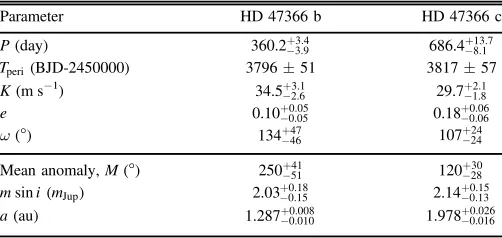
Parameter HD47366 b HD47366 c

P(day) 363.3-+2.42.5 684.7-+4.95.0

Mean anomaly(°) 288.7±75.3 93.5±35.4

Tperi(BJD-2450000) 122-+5571 445-+6255 K(m s−1) 33.6-+2.83.6 30.1-+2.02.1 e 0.089-+0.0600.079 0.278-+0.0940.067

ω(°) 100-+71100 132-+2017

msini(mJup) 1.75+-0.170.20 1.86-+0.150.16

collide with one another, are ejected from the system, or collide with the central body.

In the case of HD47366, the initial orbital parameters of the inner planet, HD47366 b, were held fixed. Our motivation for holding planet b’s parameters fixed was that the parameters of planet b are the better constrained of the pair, so by varying the less well-defined planet, we survey a larger part of parameter space for the systems potential properties. If we instead opt to hold planet cfixed, with its slightly higher orbital eccentricity, we should expect a lower overall likelihood of a stable system configuration being found. We therefore tested realizations of the outer planet, HD47366 c, incrementally adjusting the values of semimajor axisa, orbital eccentricitye,ωand mean anomaly, to probe a±3σ range around its best-fit orbital parameters. To cover the 3σparameter space, we test 41 unique values ofaand e, i.e., at each point in semimajor axis space, we test 41 unique values of orbital eccentricity. For each of those locations ina–e space, we tested 15 unique values ofω, withfive unique values of mean anomaly tested for each uniqueωexamined. This gave a grid of 41×41×15×5=126,075 simulations.

We have assumed that the two planets are on co-planar orbits. This assumption is based on knowledge of the architectures of known multiple systems (Lissauer et al. 2011; Fang & Margot 2012). It also provides a limiting case of maximum potential stability for the system (i.e., we are looking to maximize the opportunity for the system to yield dynamically feasible solutions that do not require mutual retrograde motion). We have also used the orbital parameters of the inner planet fixed at their best-fit values. This tacitly assumes that the inner planet has the better constrained orbit of the pair because it has the shorter orbital period and was thus better sampled by the radial velocity observations.

In addition to the contextual maps for the system, we performed an additional 126,075 simulations of potential architectures for the two planets involved, following the methodology laid out in Wittenmyer et al.(2017a), also using MERCURY for the n-body dynamical simulations. From the

MCMC chain obtained by our re-fitting procedure

(Section 3.2), we populated three “annuli” in c2 _space corresponding to the ranges 0 to 1σ, 1 to 2σ, and 2 to 3σ from the best fit. Each annulus contained 42025 solutions drawn from the MCMC chain (107iterations). The innermost annulus was drawn from the lowest 68.3% of allχ2values, the middle annulus contained the next best 27.2% of values, and the outer annulus contained the worst 4.5% of solutions (i.e., those falling 2–3σaway from the bestfit).

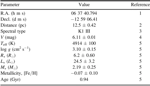
The results for our contextual simulations can be seen in Figure 1. It is immediately apparent that the best-fit solution lies in an a region of significant instability, and that the stable regions lie more beyond that bounded by the published 1σ uncertainties on the solution. Typically, stable solutions require an eccentricity for HD47366 c below ∼0.2. A region of moderate stability extends to high eccentricity at a∼1.94 au, the location of the mutual 2:1 mean-motion resonance between the two planets. However, at the eccentricity of the nominal best-fit solution, this region still only offers sufficient dynamical protection to yield mean lifetimes of the order of one million years. The results of our simulations of planet pairs around the best-fit solution fromS16are shown in Figure2.

These results are complemented by those shown in Figure 2, which presents the outcomes of our simulations of planetary solutions that fit the observational data to a given level of

precision. In thatfigure, the left-hand panels show the lifetimes of simulations for solutions that provided afit to the observational data within 1σof the best-fit, while the right-hand panels present solutions that fell within 3σ of the best-fit outcome. It is immediately apparent that very few of the systems tested proved dynamically stable on multi-million year timescales. Those that did were all found in scenarios that featured orbital eccentricities of less than 0.1 for both planets in the system. This is not a great surprise, as reducing the eccentricity of the orbits of a given planet pair while keeping all other variables constant will increase the distance between the planets at their closest approach, and therefore lessen the impact of mutual encounters on the system’s long-term stability. It should also be noted that no solutions were found that placed the two planets in mutual mean-motion resonance—ruling out the mutual 2:1 mean-motion resonance as a source of stability for the system.

As a further illustration of the S16 orbital solution, the results of our dynamical simulations for best-fit architecture proposed inS16are shown in Figure3. In these plots, we show the evolution of the semimajor axis and orbital eccentricity of the two planets as a function of time, along with a schematic plot of the proposed system architecture. It is quite self evident that the system as proposed in that work hits dynamical instability very quickly, after a period of under 10000 years.

Taken in concert, the results of our dynamical analysis suggest that the system as published in S16 is unlikely to be dynamically feasible. The observational data, however, do show two strong signals, and so it seems highly likely that the proposed planets really exist. Therefore, we revisit the fitting process for the system, to see whether the data could be fit equally well by any alternative solutions.

3.2. Re-fitting the Data

of physics to include (Chambers 1999; Laughlin & Chambers 2006). We have carried out a comparative Levenberg– Marquardt and Bayesian data analysis on a binned data set. For both modeling techniques, our analysis includes the full three-body gravitational interactions, from which we robustly derive a best-fit solution for the architecture of the system.

We have adopted the stellar mass of 2.19M_e derived in Wittenmyer et al.(2016b). As S16used 1.81M_e, this simply changes the scale of the system but does not affect the overall dynamical behavior.

Prior to modeling, we binned the data on dates with multiple successive observations, adopting the weighted mean value of the velocities in each visit. The error bar of each binned point was calculated as the quadrature sum of the r.m.s. about the mean and the mean internal uncertainty.

3.2.1. Levenberg–Marquardt Approach

In the first approach, we use the Runge–Kutta integrator within SYSTEMIC (Meschiari et al. 2009). The SYSTEMIC Console has the ability to account for interactions between planets to produce a self-consistent Newtonianfit. We use this fourth/fifth-order Runge–Kutta approach with adaptive time-step control to model the planets in the HD47366 system. Given the degree to which the planets “talk”to each other, as evidenced by our initial dynamical simulations, we felt it prudent to adopt this fitting technique. Since SYSTEMIC can

onlyfit a maximum offive data sets simultaneously, we merged the CES-O and CES-N data by applying the 24.7ms−1relative velocity offset between them as obtained byS16.

The best-fit results are given in Table3, and the orbitfits are shown in Figure4. Parameter uncertainties are obtained from a MCMC chain with 107steps, with the quoted 1σuncertainties representing the range between the 15.87 and 84.13 percentiles of the posterior distribution. The reduced χ2is 1.35 and the residual r.m.s. about the fit is 11.4ms−1, as compared to the Keplerianfit obtained byS16(r.m.s.=14.7 ms−1and reduced

χ2₌

1.0 by construction).

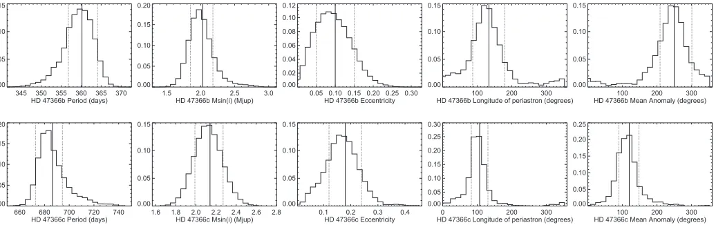
The posterior distributions of parameters for the two planets are shown in Figure5. Modeling the binned data, wefind the overall fit has improved in r.m.s. scatter compared to that of S16, and the posterior probability distributions are now unimodal. Our re-fit also results in a lower eccentricity for the outer planet; a critical criterion for dynamical stability (and hence viability)of the HD47366 system.

3.2.2. Bayesian Approach

In our second effort, we obtained posterior distributions of the HD47366 system’s orbital parameters utilising the Markov Chain Monte Carlo(MCMC)Bayesian code Exoplanet Mcmc Parallel tEmpering Radial velOcity fitteR6(ASTROEMPEROR; Figure 2.The dynamical stability ofS16ʼs previously published solution for the HD 47366 planets, as a function of the largest initial eccentricityfit to HD 47366b and c, and the ratio of their orbital semimajor axes. The color bar shows the goodness offit of each solution tested, with the left plot showing only those results within 1σ of the best-fit case, and the right plot showing all solutions tested that fell within 3σof that scenario. In the online version of this paper, the same plot is available in animated format. The animatedfigure lasts 40 s, and shows the 1σand 3σdistribution of points(equivalent to left and right panels on each line)from a changing perspective rotating around thez-axis(log(Lifetime)). These animations help illustrate the regions of parameter space that are more dynamically stable.

(An animation of thisfigure is available.)

6

J. S. Jenkins & P. A. Peña 2018, in preparation). As described in Wittenmyer et al. (2017b), ASTROEMPEROR utilizes thermodynamic integration methods(Gregory2005)following an affine invariant MCMC engine, performed using the PYTHON EMCEE package (Foreman-Mackey et al. 2013). Using an affine invariant algorithm such as EMCEE allows the MCMC analysis to perform equally well under all linear transformations consequently being insensitive to covariances among the fitting parameters (Foreman-Mackey et al. 2013). First-order moving average models are used within

ASTROEMPEROR to measure the correlated noise within the radial velocity measurements. A model selection is performed automatically byEMPEROR, whereby an arbitrary Bayes Factor value offive is required. This means a threshold probability of 150 is needed for a more complex model to be favored over a less complex one. The ASTROEMPEROR code also automati-cally determines which of the orbital parameters, such as period and amplitude, are statistically significantly different from zero, with the Bayesian information criterion (BIC), Akaike information criterion (AIC) and maximum a posteriori prob-ability (MAP) estimate values calculated for each planetary signal. Flat priors are applied to all parameters except for the eccentricity and jitter priors that are folded Gaussian and Jeffries, respectively.

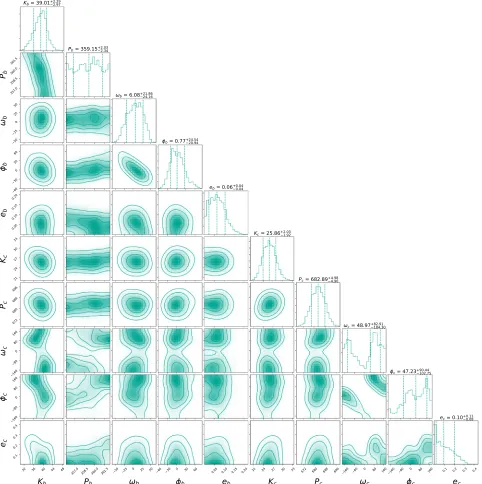
For our particular analysis, the “burn-in”chains were 3.75 million iterations long(5 temperatures, 150 walkers, and 5000 steps)with another 7.5 million chains exploring the parameter space thereafter (10000 steps instead of 5000). ASTROEM-PERORwas implemented in an unbounded manner, from zero to two planetary signals, giving flexibility for the program to discover global minima within the parameter space. The results of theASTROEMPERORanalysis are illustrated in Figure6by a corner plot, summarized in Table4, and the BIC for eachfit is given in Table5. Table4ʼs results are based upon the posterior distribution’s median value and the quoted 1σ values representing the 15.87 and 84.13 percentiles. The one-dimensional(1D)histograms of the Bayesian parameterfitting shows the fits are generally well behaved and are relatively Figure 3.Here we illustrate the instability of theS16orbital solution as demonstrated by our dynamical simulations. Left:a schematic plot of the orbital evolution of planets b and c showing thefinal complete orbit of innermost planet, HD47366b, prior to the point at which instability occurs. Showing the entire evolution of the planets for thefirst1700 years is just a clump of overlapping, precessing orbits. This schematic just shows the lead up to the moment of instability. In this plot, the red dot and line denote the position of HD47366c and its orbit, while the blue dot and line denote the position of HD47366b and its orbit. Middle:the semimajor axis evolution prior to instability(vertical dashed line). The red line denotes the semimajor axis of HD47366c, while the blue line denote the semimajor axis of HD47366b. Shaded regions denote the apastron and periastron distances at each time interval for the two planets. Right:the eccentricity evolution of the two planets until instability occurs(vertical dashed line). The red line denotes the eccentricity of HD47366c, while the blue line denotes the eccentricity of HD47366b.

Table 3

Orbital Parameters for the HD47366 System Based on Levenberg–Marquardt Analysis

Parameter HD47366 b HD47366 c

P(day) 360.2-+3.93.4 686.4-+8.113.7

Tperi(BJD-2450000) 3796±51 3817±57

K(m s−1) 34.5-+2.63.1 29.7-+1.82.1 e 0.10-+0.050.05 0.18-+0.060.06

ω(°) 134-+4647 107-+2424

Mean anomaly,M(°) 250-+5141 120-+2830

msini(mJup) 2.03+-0.150.18 2.14-+0.130.15

a(au) 1.287-+0.0100.008 1.978-+0.0160.026

Note.The time of periastron passage is afit parameter; mean anomaly, mass

msini, and semimajor axisaare derived parameters.

mono-modal. There is general good agreement between the values for the orbital parameters of the planets determined through both the Levenberg–Marquardt and Bayesian analyses of the data.

3.3. Dynamical Simulations of the New Solution

With a new solution model available for the HD47366 system, we repeated our earlier dynamical analysis. Our contextual runs again featured a hypercubic grid of 126,075 initial conditions ina–e–ω–Mspace, and our planet-pair cloud simulations again tested an additional 126,075 solutions, centered on our newly found local minimum in χ2-space.

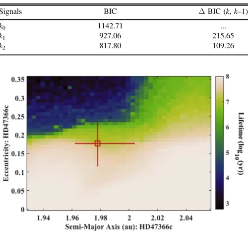
The results of our contextual simulations for this new solution can be seen in Figure 7. As a result of the new, reduced orbital eccentricity for this solution, the bestfit to the data now lies on the edge of a broad region of dynamical stability. A significant fraction of the individual trials within the 1σuncertainty range on the solution were found to survive for the full 100Myr duration of our integrations, a result in stark contrast with those we performed of theS16solution. We note, in passing, that while the general structures visible in Figure7 are the same as those in Figure 1, the broad expanse of solutions within the 2:1 mean-motion resonance between the two planets (to the right of the plot) now exhibits somewhat improved stability. This is the result of the broader range ofω andMvalues sampled by the new solution, which increases the likelihood of the two planets being trapped in a stable resonant configuration in our runs.

The results of our simulations of planet pairs around the best-fit solution are shown in Figure8. It is immediately apparent that a far greater number of tested two-planet scenarios prove dynamically stable in the simulations compared to those based on the S16 solution (shown in Figure 2). Again, the stable solutions cluster toward lower maximum eccentricities—but the stable region now extends to markedly higher eccentricities. A broad island of stability is clearly visible at eccentricities less than

∼0.2, and for semimajor axis ratios between∼0.63 and∼0.66. In a

a

1 2

space, the 2:1 mean-motion resonance would be centered on a value of 0.63, with values greater than this revealing pairs of orbits whose periods are more similar to one another. Even values of a

a

1 2

of 0.66 are still very close to the

center of the 2:1 mean-motion resonance—indeed, such orbits would exhibit a period ratio of approximately 13:7(or 1.86:1)

—well within the breadth of the influence of the 2:1 mean-motion resonance. In other words, it seems likely that the stable solutions resulting from our new analysis are facilitated by the influence of that resonance—which would also explain how stable orbits can be maintained up to moderately large orbital eccentricities.

3.4. Computation of Dynamical MEGNO Maps

In an attempt to further understand the dynamics of the two planets, we have applied the MEGNO7 technique (Cincotta & Simó 2000; Goździewski et al. 2001; Cincotta et al. 2003)for the numerical assessment of chaotic/quasi-periodic orbits in a multi-body dynamical system and has found wide-spread applications within the astro-dynamics community (Goździewski et al. 2001; Hinse et al. 2010, 2014; Contro et al. 2016; Wood et al. 2017). The MEGNO technique is especially useful to detect the location of orbital resonances. In summary, MEGNO (often denoted as á ñY ) quantitatively measures the degree of stochastic behavior of a nonlinear dynamical system. Following the definition of MEGNO (Cincotta & Simó 2000), a dynamical system that evolves quasi-periodically, the quantity á ñY will asymptotically approach the value of 2.0 for t ¥. In case of quasi-periodicity, the orbital elements for a given body are bounded and their time evolution described by a few number of characteristic frequencies. For a chaotic time evolution the quantityá ñY will diverge away from 2.0. An important point to make is that quasi-periodicity or regular dynamics can only be demonstrated numerically up to the considered integration time. Our results were obtained by using a modified version of the Fortran-based μFARM8code (Goździewski et al. 2001, 2008; Goździewski 2003). The package utilizes OpenMPI9 and is capable of spawning a large number of single-task parallel jobs on a given super-computing facility. The package main functionality is the computation of MEGNO over a grid of Figure 5.Posterior probability distributions for HD47366b(top)and HD47366c(bottom)from our re-fit of orbital parameters using the combined Levenberg– Marquardt and MCMC analysis. Parameters are(in order left to right)orbital period(P), line-of-sight mass(msini), eccentricity(e), longitude of periastron(ω), and

mean anomaly(M). The distributions are well behaved, and the simultaneous best-fit values for the parameters of both planets lie close to the peak of their respective probability distributions.

7 _{Mean Exponential Growth factor of Nearby Orbits.}

8

https://bitbucket.org/chdianthus/microfarm/src

9

initial values in orbital elements for a n-body problem. The equations of motion and associated variational equations are solved using and effective Gragg-Bulirsh-StoerODEX10 extra-polation algorithm with step-size control(Hairer et al.1993).

The choice of initial conditions is identical as described in Section3.1. For a given(ac,ec)grid-point of the outer planet, a sub-set of various w-M parameter combinations is consid-ered within their calculated 1σ uncertainty. We refer to Goździewski & Migaszewski (2014) for a similar approach in their Section 4.5. As for the dynamical study in the previous section, wefixed the inner planet to its best-fit parameters. The host-star mass was set to 2.19M_e. The single grid-point

maximum integration time was set to 106years due to limited computation resources available. The MEGNO integration corresponds to over 5×105orbital periods of the outer planet and hence likely captures the secular time period of the system. For each (ac,ec) parameter pair, we recorded the minimum value ofá ñY for all triedwc-Mcparameter combinations. The minimum value ofá ñY is then used to generate a dynamical map over(ac,ec)space. This approach ensures that we detect quasi-periodic regions for the probed parameter pairs. How-ever, this approach does not provide information on a specific wc-Mc combination that resulted in a minimum ( quasi-periodic)value ofá ñY .

We present our results in Figure 9. The(ac,ec) map, to a large degree, agrees with the lifetime map shown in Figure7. Figure 6.Bayesian posterior distributions of HD47366 b and HD47366 c’s orbital parameters derived fromASTROEMPEROR. From left to right(top to bottom), the parameters areKb,Pb,ωb,fb,eb,Kc,Pc,ωc,fc, andec. Credible intervals are denoted by the solid contours with increments of 1σ. Each 1D histogram exhibits dashed

lines, displaying the median and±σvalues(also displayed above for clarity).

10

The two independent results complement each other and provide confidence in the numerical results obtained. Overall, the considered (ac,ec) region is characterized by three areas: (i)an area of general orbital instability mainly in the upper left corner,(ii)an area of stability for low-ecorbits, and(iii)an area

characterized by an intermediate stability/instability. We point out that the computed MEGNO map considers a somewhat larger range in (ac,ec) space as compared to Figure 7. The newly determined LM+MCMC bestfit places the outer planet on the transition region between quasi-periodic (stable) and chaotic dynamics. Long-term orbital stability is still ensured considering the (ac,ec) parameter uncertainty range for the

outer planet. Low eccentric orbits are preferred prolonging the system’s lifetime.

3.5. 2:1 Near-resonant Dynamics

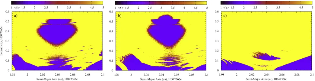
We point out a fourth characteristic in Figure9. The region around(ac,ec)=(2.05 au, 0.35)exhibits quasi-periodic orbits for some of the probed wc-Mc parameter combinations (shown as black dots in Figure10). We find that the overall dynamics of the region is characterized by the 2:1 mean-motion resonance. The results from our dynamical analysis therefore point toward a two-planet system in a near-resonant orbital architecture. To further characterize the nature of this resonance we have calculated a dynamical MEGNO map over the space

w

(Mc, c) for a fixed (ac,ec)=(2.05 au, 0.367). The result is shown in Figure 10. A total of four stable islands are found. Each corresponds to a particular initial orbital geometry of the two planets resulting in quasi-periodic dynamics. A stable system in 2:1 resonance (for (ac,ec)=(2.05 au, 0.367)) is achieved for particular initial differences in apsidal lines (wc-wb)and phases(Mc-Mb). The four islands correspond to four initial configurations resulting in a stable 2:1 resonance. In fact, some of these islands were encountered when calculating Figure 9 as part of the wc-Mc hypercube parameter scan for a chosen (ac,ec) pair. This approach is particular effective in identifying orbital resonances.

We have repeated the calculation of Figure 9 for particular w

(Mc, c)combinations corresponding to the approximate center of two libration islands in Figure 10 (shown as black star-like symbols). One particular(Mc,wc)=(300 , 50 ) pair is deliber-ately chosen to be within the chaotic region for comparison. The corresponding dynamical MEGNO maps are shown in Figure11. In comparison with Figure9, we now clearly identify the quasi-periodic island associated with the 2:1 resonance for two chosen initial configurations of apsidal line and phase differences. For the initial condition chosen from the chaotic region, wefind that the stability island now disappears as expected.

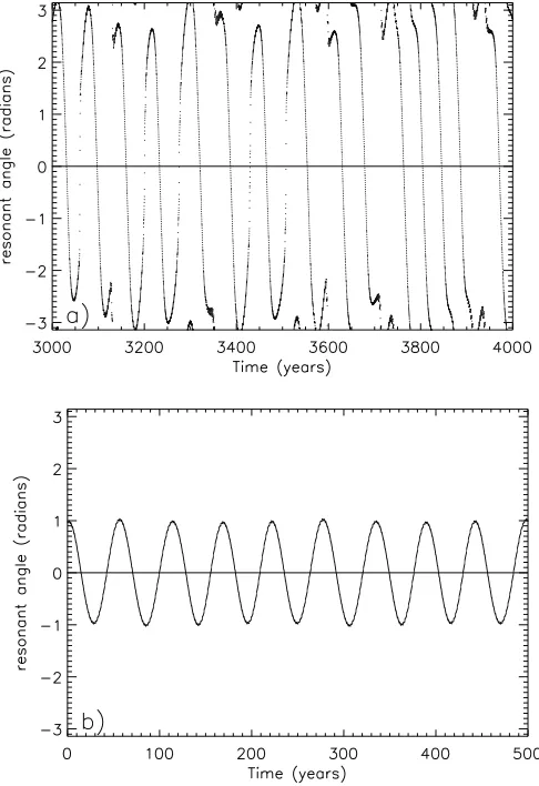
As a last exercise, we have checked the time evolution of the critical resonant angle for two particular initial conditions. The resonant angle for the 2:1 mean-motion resonance is

f=2lc-1lb-wb ( )1

whereλis the mean longitude for either planet. In Figure12, we plot this angle for the two cases: Panel (a): (ac,ec,

wc,Mc)=(2.05 au, 0.01, 259 , 28 ). Panel (b): (ac,ec,wc,

=  

) ( )

Mc 2.05 au, 0.01, 50 , 300 . From direct numerical

inte-grations using theMERCURY(Chambers 1999) integrator, we find the quasi-periodic and chaotic time evolution of the resonant angle for the two chosen initial conditions demon-strating stable and chaotic dynamics.

4. Discussion

In recent years, a number of studies have shown the importance of performing dynamical tests of newly proposed planetary systems in order to verify that the proposed systems are truly dynamically feasible (e.g., Horner et al. 2011,2018; Wittenmyer et al.2014). In this light, we performed a detailed dynamical analysis of the proposed HD47366 planetary system, as detailed in Sato et al.(2016). Our results indicated a good chance that the two-planet system proposed in that work would be dynamically unstable, and therefore raises its plausibility into question. Since the observational data clearly Table 4

Bayesian Re-fitting of the HD47366 Planetary System Through thePYTHON

PackageASTROEMPEROR

Parameter HD47366 b HD47366 c

P(day) 359.15-+2.342.03 682.85-+4.904.98

fa_{(°) 0.77} -+

20.9424.54 47.23-+102.7590.44

K(m s−1) 39.01-+2.972.29 25.86-+1.922.03

e 0.06-+0.040.04 0.10-+0.080.11

ωa_{(°) 6.08}

-+

24.1621.86 48.97-+184.3082.91

msini(mJup) 2.30-+0.180.13 1.88-+0.140.12

a(au) 1.28-+0.060.05 1.97-+0.090.08

Notes. a

fis a measured parameter defined in ASTROEMPEROR asf=M- pt P

2

, related to the mean anomaly(M), orbital period(P)and epoch time(t).

Table 5

Bayesian Information Criterion(BIC)Statistic for EachASTROEMPEROR Signal Fit from a Zero(k0)to Two Planet Fit(k2)

Signals BIC ΔBIC(k,k–1)

k0 1142.71 ...

k1 927.06 215.65

k2 817.80 109.26

show evidence for two strong signals, we chose to perform a fresh analysis of that data, in order to determine whether a dynamically stable solution could be found that is an adequate fit to the observations.

To fully characterize the proposed system, we examined a binned data set of radial velocity observations of the two-planet HD47366 system using two independent methods to deter-mine the best-fit parameters of the system, under the assumption of co-planar orbits. We find that the system properties determined by each method are generally consistent. For HD47366 c, all the orbital parameters agree within uncertainties. For HD47366 b, the orbital angles ω and M determined by each method are not consistent with each other. However, the large uncertainties on those values(<90°)makes the significance of this discrepancy small (<3−σ), and we conclude that the results of the separate analyses are therefore in agreement.

Once we had obtained our new solution for the two-planet system, we performed a fresh dynamical analysis, examining whether our solution offered greater prospects for stability than that proposed inS16. In strong contrast to that earlier work, we found that our new solution resulted in a large number of potentially stable scenarios, all of which offered an excellentfit to the observational data. Those solutions nestled close to the location of the mutual 2:1 mean-motion resonance between the two proposed planets. This enhanced stability affords us greater confidence in the validity of our new solution.

The orbital parameters of the best-fitting model produce an architecture with the outer planet having an orbital period∼1.9 times that of the inner planet. Multi-planet systems discovered by Keplerexhibit a significant pile-up at orbital periods close to, but Figure 8.The dynamical stability of our revised solution for HD47366ʼs planets, as a function of the largest initial eccentricityfit to HD 47366b and c, and the ratio of their orbital semimajor axes. The color bar shows the goodness offit of each solution tested, with the left plot showing only those results within 1σof the best-fit case, and the right plot showing all solutions tested that fell within 3σof that scenario. In the online version of this paper, the same plot is available in animated format. The animatedfigure lasts 40 s, and shows the 1σand 3σdistribution of points(equivalent to left and right panels on each line)from a changing perspective rotating around thez-axis(log(Lifetime)). These animations help illustrate the regions of parameter space that are more dynamically stable.

(An animation of thisfigure is available.)

Figure 9.Dynamical MEGNO map considering the(ac,ec)space for the outer planet HD47366c based on the LM+MCMC modeling work. We plot the minimum value of MEGNO. Quasi-periodic orbits have log₁₀Ymin0.3. See

outside of, the 3:2 and 2:1 resonances with an inner planet(Wang & Ji2014), typically inferred to be a relic of planetary migration in the presence of an accreting circumstellar disk. Given the proximity of our new solution to the 2:1 mean-motion resonance, it seems plausible that the HD47366 planetary system can be added to the catalog of such compact planetary systems.

As HD47366 evolves off the main sequence and undergoes significant mass loss, its planetary system will be destabilized. The cause of this destabilization are the tides raised by the planets on the puffed up star. Tidal forces act to damp the planet’s semimajor axis and eccentricity. The two possible outcomes of this process are either engulfment by the host star or evaporation into interstellar space, depending on the initial semimajor axis and mass of the planetary companion (Mustill & Villaver 2012). Modeling has shown that tidal effects become important when the periastron distance of the planet approaches between two and three stellar radii. In the case of HD47366, both planets have semimajor axes small enough that they will likely be subject to tidal forces as the host star evolves. HD47366ʼs planets will therefore undergo rapid orbital decay and be engulfed during its post-main-sequence evolution, similar to the expected fate of the eccentric gas giant around HD76920(Wittenmyer et al.2017a).

5. Conclusions

We have performed a thorough dynamical reanalysis of the planetary system proposed to orbit the star HD47366 inS16.

Our simulations cast doubt on the dynamical feasibility of the solution proposed in that work. As a result, we have performed a detailed reanalysis of the available observational data for the system and have used that to produce an improved solution for the proposed two-planet system.

Through our Levenberg–Marquardt reanalysis of the two-planet system proposed around HD47366, we have demon-strated that a low(er) eccentricity orbital solution exists compared to that proposed byS16. This solution is shown to be dynamically stable for periods up to 100Myr and is comparable to the orbital parameters derived by our Bayesian reanalysis of the system.

We present this work as a cautionary tale in exoplanet dynamics—the best-fit solution derived from Keplerian modeling of radial velocities may only be a local one, particularly if the resulting solution requires contrived architectures to be stable over periods comparable to the lifetime of the host star. By expanding the parameter space explored in the fitting process, we have determined a much more dynamically plausible solution for the architecture of the HD47366 system.

The authors thank the anonymous referee for their constructive criticism.

This research has made use of the SIMBAD database, operated at CDS, Strasbourg, France.

Figure 10.Dynamical MEGNO maps considering the(Mc,wc)space of the outer planet for afixed(ac,ec)=(2.05 au, 0.367). The top panel shows the chosen initial

w

(Mc, c)parameter range. Black star-like symbols are at(Mc,wc)=(210 , 26 ),(Mc,wc)=(28 , 259 )and(Mc,wc)=(300 , 50 ). The black dots indicate our probeda- -e w-M hypercube. The bottom panel shows the initial conditions relative to the(best-fit)initial(Mb,wb)=(250 , 134 )of the inner planet.

This research has made use of NASA’s Astrophysics Data System.

This research has been supported by the Ministry of Science and Technology of Taiwan under grants MOST104-2628-M-001-004-MY3 and MOST107-2119-M-001-031-MY3, and Academia Sinica under grant AS-IA-106-M03.

Software:SYSTEMIC (Meschiari et al. 2009), ASTROEM-PEROR(https://github.com/ReddTea/astroEMPEROR), MAT-PLOTLIB(Hunter 2007),MERCURY(Chambers 1999),EMCEE (Foreman-Mackey et al.2013).

ORCID iDs

J. P. Marshall https://orcid.org/0000-0001-6208-1801 R. A. Wittenmyer https://orcid.org/0000-0001-9957-9304 J. Horner https://orcid.org/0000-0002-1160-7970

J. Clark https://orcid.org/0000-0003-3964-4658 M. W. Mengel https://orcid.org/0000-0002-7830-6822 T. C. Hinse https://orcid.org/0000-0001-8870-3146 S. R. Kane https://orcid.org/0000-0002-7084-0529

References

Bakos, G. Á., Lázár, J., Papp, I., Sári, P., & Green, E. M. 2002,PASP,114, 974 Borucki, W. J., Koch, D., Basri, G., et al. 2010,Sci,327, 977

Bowler, B. P., Johnson, J. A., Marcy, G. W., et al. 2010,ApJ,709, 396 Butler, R. P., Vogt, S. S., Laughlin, G., et al. 2017,AJ,153, 208 Chambers, J. E. 1999,MNRAS,304, 793

Cincotta, P. M., Giordano, C. M., & Simó, C. 2003,PhyD,182, 151 Cincotta, P. M., & Simó, C. 2000,A&AS,147, 205

Contro, B., Horner, J., Wittenmyer, R. A., Marshall, J. P., & Hinse, T. C. 2016,

MNRAS,463, 191

Coughlin, J. L., Mullally, F., Thompson, S. E., et al. 2016,ApJS,224, 12 Durkan, S., Janson, M., & Carson, J. C. 2016,ApJ,824, 58

Fang, J., & Margot, J.-L. 2012,ApJ,761, 92

Fischer, D. A., Marcy, G. W., & Spronck, J. F. P. 2014,ApJS,210, 5 Foreman-Mackey, D., Hogg, D. W., Lang, D., & Goodman, J. 2013,PASP,

125, 306

Goździewski, K. 2003,A&A,398, 315

Goździewski, K., Bois, E., Maciejewski, A. J., & Kiseleva-Eggleton, L. 2001,

A&A,378, 569

Goździewski, K., Breiter, S., & Borczyk, W. 2008,MNRAS,383, 989 Goździewski, K., & Migaszewski, C. 2014,MNRAS,440, 3140 Gregory, P. C. 2005,ApJ,631, 1198

Hairer, E., Nørsett, S. P., & Wanner, G. 1993, Solving Ordinary Differential Equations I. Non-stiff Problems(2nd ed.; Berlin: Springer)

Hinse, T. C., Christou, A. A., Alvarellos, J. L. A., & Goździewski, K. 2010,

MNRAS,404, 837

Hinse, T. C., Horner, J., & Wittenmyer, R. A. 2014,JASS,31, 187 Høg, E., Fabricius, C., Makarov, V. V., et al. 2000, A&A,355, L27 Horner, J., Hinse, T. C., Wittenmyer, R. A., Marshall, J. P., & Tinney, C. G.

2012,MNRAS,427, 2812

Horner, J., Marshall, J. P., Wittenmyer, R. A., & Tinney, C. G. 2011,MNRAS, 416, L11

Horner, J., Wittenmyer, R. A., Hinse, T. C., et al. 2013,MNRAS,435, 2033 Horner, J., Wittenmyer, R. A., Hinse, T. C., & Marshall, J. P. 2014,MNRAS,

439, 1176

Horner, J., Wittenmyer, R. A., Wright, D. J., et al. 2018, AJ, 795, 85 Houk, N., & Smith-Moore, M. 1988, Michigan Catalogue of Two-dimensional

Spectral Types for the HD Stars, Vol. 4 (Ann Arbor, MI: Dept. of Astronomy, Univ. of Michigan)

Hunter, J. D. 2007,CSE,9, 90

Janson, M., Brandt, T. D., Moro-Martín, A., et al. 2013,ApJ,773, 73 Jenkins, J. S., Jones, H. R. A., Tinney, C. G., et al. 2006, MNRAS, 372,

163

Johnson, J. A., Clanton, C., Howard, A. W., et al. 2011,ApJS,197, 26 Johnson, J. A., Fischer, D. A., Marcy, G. W., et al. 2007,ApJ,665, 785 Jones, M. I., Jenkins, J. S., Brahm, R., et al. 2016,A&A,590, A38 Lannier, J., Lagrange, A. M., Bonavita, M., et al. 2017,A&A,603, A54 Laughlin, G., & Chambers, J. 2006, ISSIR,6, 233

Lissauer, J. J., Ragozzine, D., Fabrycky, D. C., et al. 2011,ApJS,197, 8 Marshall, J., Horner, J., & Carter, A. 2010,IJAsB,9, 259

Meschiari, S., Wolf, A. S., Rivera, E., et al. 2009,PASP,121, 1016 Mustill, A. J., Marshall, J. P., Villaver, E., et al. 2013,MNRAS,436, 2515 Mustill, A. J., Veras, D., & Villaver, E. 2014,MNRAS,437, 1404 Mustill, A. J., & Villaver, E. 2012,ApJ,761, 121

Pepper, J., Pogge, R. W., DePoy, D. L., et al. 2007,PASP,119, 923 Perryman, M. A. C., Lindegren, L., Kovalevsky, J., et al. 1997, A&A,323,

L49

Pollacco, D. L., Skillen, I., Collier Cameron, A., et al. 2006,PASP, 118, 1407

Reffert, S., Bergmann, C., Quirrenbach, A., Trifonov, T., & Künstler, A. 2015,

A&A,574, A116

Sato, B., Omiya, M., Wittenmyer, R. A., et al. 2013,ApJ,762, 9 Sato, B., Wang, L., Liu, Y.-J., et al. 2016,ApJ,819, 59 van Leeuwen, F. 2007,A&A,474, 653

Wang, L., Sato, B., Zhao, G., et al. 2012,RAA,12, 84 Wang, S., & Ji, J. 2014,ApJ,795, 85

Wittenmyer, R. A., Horner, J., & Marshall, J. P. 2013,MNRAS,431, 2150 Wittenmyer, R. A., Horner, J., Marshall, J. P., Butters, O. W., & Tinney, C. G.

2012a,MNRAS,419, 3258

Wittenmyer, R. A., Horner, J., Mengel, M. W., et al. 2017a,AJ,153, 167 Wittenmyer, R. A., Horner, J., & Tinney, C. G. 2012b,ApJ,761, 165 Wittenmyer, R. A., Johnson, J. A., Butler, R. P., et al. 2016a,ApJ,818, 35 Wittenmyer, R. A., Jones, M. I., Horner, J., et al. 2017b,AJ,154, 274 Wittenmyer, R. A., Jones, M. I., Zhao, J., et al. 2017c,AJ,153, 51 Wittenmyer, R. A., Liu, F., Wang, L., et al. 2016b,AJ,152, 19 Wittenmyer, R. A., Tan, X., Lee, M. H., et al. 2014,ApJ,780, 140 Wood, J., Horner, J., Hinse, T. C., & Marsden, S. C. 2017,AJ,153, 245 Figure 12.Time evolution of the critical resonance angle. In the top panel, the