PP backward elastic scattering between 0.70 and 2.37 GeV/c

BE'J'WEJ..;N 0. 70 J\ND 2. 3~( GEV /C

'l'hesis by

,John K. Yoh

In Partial F'ulfilllnent of the Requirements

For

the Degree of Doctor of Philosophy

Ca.l.i..1."ornia Institute of 'l'echnology Pasadena, California

1970

ii

ACKNOWLEDGMENTS

The author wishes to thank his advisor, Professor Barry Barish, for advice and encouragement. The author also wishes to extend his gratitude to Professors Jerome Pine and Alvin V. Tollestrup for help and advice during and after the experiment. The author is also in-debted to the other members of the collaboration who are involved with the experiment. These include Mr. Howard Nicholson of Caltech,

Drs. Alan S. Carroll and Robert H. Phillips of Brookhaven National Laboratory, and Claude Delorme, Fred Lobkowicz, Adrian C. Melissinos and Yori Nagashima of the University of Rochester.

The author is also indebted to the support personnel of the three institutions, in particular to Messrs William Friedler, Hans Grau and Jack Sanders. The aid and support from the BNL computer center staff and the AGS EAO group are also gratefully acknowledged.

A BS'f RAC'!'

pp backward elastic scattering has been measured for the

-cos 0 region between -

1.00

and -

0.88

and for the incident p

cm

laboratory momentum region between

0. 70

and

2.37

GeV/c. These

measurements, done in intervals of approximately

0.1

GeV/c, have been performed at the Alternating Gradient Synchrotron at Brookhaven

National Laboratory during the winter of

1968.

The measured dif-ferential cross sections, binned in cos

e

intervals of

0.02,

have

cm

statistical errors of about

10%.

Backward dipping exists below

0.95

GeV/c and backward peaking above

0.95

GeV/c. The

180°

differen-tial cross section extrapolated from our data shows a sharp dip centered at 0.9.5 GeV/c and a broad hump centered near 1.4 GeV/c. Ou1· dat.:i have been int0rpretl>.<l in terms of resonance effects and in

TABLE OF CONTENTS

CHAPTER I: INTRODUCTION

CHAPTER II: EXPERIMENTAL APPARATUS AND METHODS (a) Introduction and experimental layout (b) Beam target and magnet

8 14 (b-i) Beam and p identification and counting 14

(b-ii) Target 24

(b-iii) Magnet and momentum measurement (c) Fast counters and logic

(c-i) Introduction

(c-ii) Trigger counters, logic and rates (c-iii) Counter bits -- scintillation counter

(c-iv) (c-v)

information for analysis

The gas threshold Cherenkov counter The forward outgoing particle

time-of-flight system

(d) Recording and monitoring of data

24

28

28

30

36

37

42 44

(d-i) Introduction 44

(d-ii) Wire spark chambers and the recording

of digitized spark positions 44 . (d-iii) PDP-8 computer and interface system of

recording the data 50

(d-iv) Data recording -- summary of data taking procedure

(d-v) The contents of the data recorded

51

58 (d-vi) Monitoring of the data taking 59 (e) Evaluation of the apparatus and data taking system 60

CHAPTER III: ANALYSIS OF THE DATA (a) Introduction

(b) Reconstruction of events

65 66

(b-i) Introduction 66

(b-ii) The finding of event tracks from the

(b-iv) (b-v)

Reconstruction inefficiency

Analysis of triggered events which fail the reconstruction process

(c) SP.l.ect:ion

or

backward c•hrnt:ic pp ('Vf'nts (c-1) Introduction

(c-ii) Topology selection criterion (c-iii) Reconstructed vertex criterion

(c-iv) Velocity criterion

(c-v) Momentum criterion

(d) Corrections to the normalization

(e) Monte Carlo of the apparatus acceptance

(f) Calculation of the differential cross sections and errors

72 74

75

7 ') 77 80

82

84 85 90 94 (g) Summary and assessment of the analysis procedure

96

CHAPTER IV: RESULTS-- PP BACKWARD ELASTIC DIFFERENTIAL CROSS

SECTIONS

(a) Differential cross section for each angular bin 103 (b) The 180° des and slope extrapolated from our data 103

(c) Comparison of our data with other existing data 116

(d) Features of our data 117

CHAPTER V: RESONANCES: AN INTERPRETATION OF THE DATA

(a) Introduction and the probable absence of strong

Regge u channel effects 119

(b) Resonances and the pp system: theoretical

considerations 121

(b-i) !he coupling of resonances to the

pp system 121

(b-ii) Features_of resonance contribution to

elastic pp scattering 123

(c) Other experimental and theoretical evidence for

boson resonances 130

(c-i) Other experimental evidence

(c-ii) Theoretical models predicting boson

resonances

(d) What our data say about resonances in the direct channel

130

(d-i) Narrow resonances (d-ii) Broad resonances (e) Conclusion

CHAPTER VI: DIFFRACTION, AN ALTERNATE INTERPRETATION OF THE DATA

140 142 147

(a) Introduction and motivation for this interpretation 149

(b) Spin-orbit optical model 155

(b-i) Formulation of the model 155 (b-ii) Spin-orbit optical model and our data 158 (b-iii) Assessment of the spin-orbit optical

model -- does it reproduce other

pp

elastic and polarization data? 162 (c) Diffraction dominance and pp elastic scattering 167

(c-i) Brief survey of other diffraction

type models 167

(c-ii) Features of diffraction dominance in

pp elastic scattering 168

(c-iii) Assessment of diffraction dominance and suggestion for further experimentation 169

CHAPTER VII: SUMMARY AND CONCLUSION (a) Summary

(b) Conclusion

Appendix A: Beam transport system Appendix B: Wire spark chambers

Appendix C: Inef~iciencies in reconstruction of triggered events

References

171 173 174 178

Figure Number

1.1

1. 2 1.3

2.1

2.2

2

.

3

2.4

Index of Figures

Contents

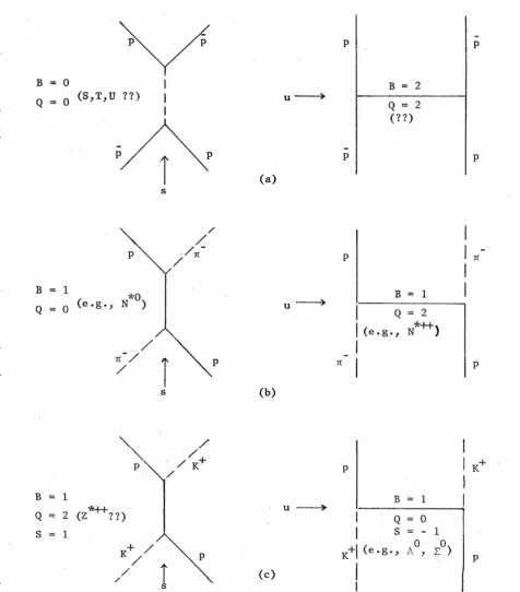
Feynman diagrams for the s and u channel

contributions to backward elastic scattering of pp, rc_p,and K+p.

re p elastic scattering at

180°

K+p backward elastic scattering data

Layout of the separated beam transport system Layout of our apparatus

Beam liquid differential Cherenkov counter Beam Cherenkov and time-of~f light curves

Page

2 4 5 10

12

17

18

2.5

Distribution of beam momentum, positions and

slopes 22

2.6

Rectangular field. model for a dipole magnet 27

2.7

Improving momentum determination using mass slit

counters

29

2.8

Triggering area in P-R space 33

2.9

The trigger logic flow chart 35

2.10

Gas threshold Cherenkov counter 39

2 .11 Cherenkov pulse-height channel distributions 40

2.12 Time-of-flight channel distributions 43

2 .13 Wire spark chamber signals and digitizer operation 47 2.14 Trigger and event recording timing diagram 53

3.1

Topology of a desired backward elastic event

68

3.2

Distribution of VD and MTD for backward elastic

events 79

3.3 (MM) 2 - . (Mp) 2 distributions for events passing and

failing velocity criterion 83

3.5

4.1

4.2

4.3

4.4

4.5

5.1

5.2

5.3

5.4

5.5

viii

Flow chart of the analysis procedure Our data in µb/sr

2 Our data in µb/GeV

0

Linearly extrapolated 180 des and slope in µb/sr

0

Linearly extrapolated 180 des and slope in µb/Gev2.

0

Exponential extrapolated 180 des and slope in µb/Gev2.

Angular momentum barrier for pp and nN systems.

Shape of the resonance contribution to the des

qq model predicted meson states

Meson states predicted by the daughter trajectory model

Resonance prediction for 180° des using total cross section resonance candidates

6.1

Forward elastic pp des and diffraction model curves

6.2

6.3

6.4

6.5

Diffraction nature of large angle pp elastic des 3-dimensional compilation of pp elastic des be low 2 GeV /c

0 Spin-orbit optical model curves of the 180 des and slope

Spin-orbit optical model curves in the region of our data

6.6 Spin-orbit optical model curves for elastic

A. l

B. l

· scattering below 1.5 GeV/c· and for polarization measurements

Beam ray trace

Wire spark chamber construction and operation

C.1 Calcomp plotter pictures of several triggered evt~nt s

97 106 107 113 114 115

124

127 137 139

145

150 153

154

159 160 164 176 179

Index of tables

Table

Number Contents Page

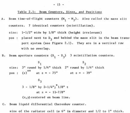
2.1 Beam counter sizes and positions 15

2.2 Beam fluxes and rates 21

2.3 Non-beam scintillation counter sizes and positions 31 2.4 Positions and sizes of the sensitive areas of

·.

the wsc

3.1 Sizes of all corrections to the normalization

3.2 Properties of the analysis and data at each momentum

4 .1

4.2

pp backward elastic des obtained in our experiment (µb/sr)

pp backward elastic des in µb/Gev2

4.3 pp 180° elastic des and slope using linear extrapolation

4.4

5.1

- 0

pp 180 elastic des and slope (exponential extrapolation)

Boson resonance candidates above twice the proton mass

46

87

99

104

105

109

111

CHAPTER I: INTRODUCTION

In the study of high energy interactions, the des (differential cross section) at extreme angles has been very useful in revealing the important mechanisms responsible for the interaction. Strong contributions from s (except s-wave), t or u channels usually lead to d cs with characteristic pea ings or dipping at k extreme angles (1.1) or with characteristic dependence on energy. In the case of elastic

scattering, the forward des is not very useful in revealing any

mechanism aside from the diffraction which dominates forward scattering. Thus, the des for elastic backward scattering is crucial to the ex-ploration of any important u channel and s channel mechanisms con-tributing to the elastic scattering. Figure 1.1 shows the Feynman diagrams corresponding to the s and u channel contributions to the backward elastic scattering of (a) pp; (b) n

-

p; and (c) K

+

p.

Away from the low energy region, s channel contribution to elastic scattering is no longer dominated by s wave. Thus, the indi-vidual partial wave amplitudes of the important terms contribute larger

(1.2)

values to the extreme angles • In the event that s channel is dominated by a particular resonance near a certain energy region, the s channel contribution to the extreme backward elastic des is charac-teristic. The size of the contribution peaks at the position of the resonance while at the same time there is backward peaking at the

f (1.3)

Figure 1.1: Feynman diagrams for the s and u channel contributions to the backward elastic scattering of (a) pp, (b) n-p.and (c) K+p.

Quantum numbers of the s and u channels are given. Possible candidates for the contributions are given in parenthesis.

p p p

B 0 _B

=

₂

Q 0

(S,T,U ??)

u~ _Q

=

₂

(

??

)

p

T

p p p

(a) s

/

/

p ./ n

-/

p n

B

=

1 _B

=

₁

*

O

Q 0 (e.g.,

N )

u ----7

I

_Q

=

₂

I

(e.g.,

N

*

++)

/

I

1(-/

r

p n

I

p

/

s (b)

/

/

p / K+ _p K+

/

B

=

1 _{B 1}

(z*++??)

u~

Q =;. 2 _{Q 0}

s

=

1

s

- 1

K+ / _p K

+I

(e.g.' /\ 0

,

L..o) p

/

1

I

/ (c)

/

[image:11.565.30.506.144.686.2]

3

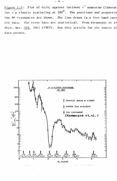
-In 1( p backward elastic scattering in the region 1.65 ·- 5.3

GeV/c(l.4), the des at 180°, shown in Figure 1.2, revealed many

sharp structures. For example, there are sharp bumps at 1688 and 1924

and a sharp dip at 2190, all of these can be attributed to resonance

effects in the direct s channel. Indeed, this set of data was useful

in indicating the properties of the resonances as well as suggesting

possible existence of a new resonance at 3245 MeV. In the backward

elastic differential cross section of other processes, it is possible

to see similar structures in the event of strong resonance contribution

from the s channel.

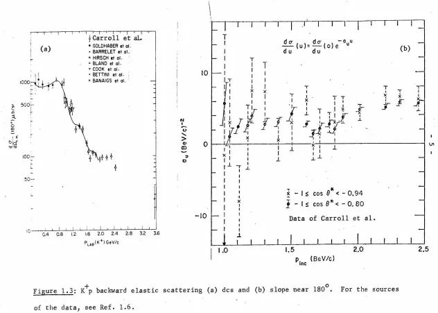
u channel effects· may also be important in the backward elastic

region. In the event that strong s channel and background

contribu-tions are absent, the u channel contribution, if it is dominated by a

single (or an exchange degenerate set of) Regge trajectories, produces

a backward elastic des (do/du, in this case) which has energy and angle

dependence of s2a (u) - 2 (l.S) where a(u) is the function corresponding

to the dominant trajectory. Thus, the do/du at u

=

0 would have as-a

dependence where a= 2 - 2a(O). At a particular s, do/du as a function

of u shows an e ba(u) d~pendence . where b is 2 in(s). These behaviors

+

are shown by

K

p backward scattering; we have plotted the do/du near

180

°

of K+p scattering as a . f unction o . f s in . Figure . l • a 3 an d th e s ope l

of do/du in Figure l.3b(l.6). The data indicate that the des is

consistent with the hypothesis that i t is. dominated by the A (and/or

y

the A , in case of exchanging degeneracy) trajectories. In this

a

particular case, there are good reasons to suspect that u channel

for

~

p elastic scattering at 180°. The positions and properties of the N* resonances are shown. The line drawn is a free hand curve of the data. The error bars are statistical. From Korrnanyos ct al ., Phys. Rev. 164, 1661 (1967). See this article for the source of other data points.

200

~;~,~00

:t, w t. ~···' ....

fl

•IO • ,,,w••,

..

,.,

v .. ::o

·4

-TT -p ELASTIC SCATTERING

~

t

llERKELEY Holland 1\ ol.(160")

f

NIMROD Du kt o\ al. (IG5•)

+

TlllS EXPEfllMENT

(Kormanyos et.al.)

2190

213

2'4~

2~

I

50 3245

l•tz,?.-1 P.<z,7.+I I 1'12_?·-I _{''·'z.?:i!____ _ _} ~r_.i_._.,

__

~

z 3 4 5

[image:13.572.68.471.60.684.2]

1000;

:; 5

00'-~ !

::l.. r

0

0 ~

' E bi v

le:

.,,

,

,,

~ 100;__ ~ 5

0

-(a)

Pi

~Carroll et al.

• GOLDHABER et ol.

• BARRELET et ol.

• HIRSCH et ol. • BLAND et ol. •COOK et al. • BETTINI et al.

o BANAIGS et al. .

~H?

?

J

1

iC; !

0.4 0.8 1.2 1.6 2.0 2.4 2.B 3.2 3.6 PLAB(K+) GeV/c

10

"'

_... I

u

...

>

Cl.I

₀

m

~ :J 0 -10

I

T I I I I I IT

1T

1

dCT dcr -o U

- ( u ) = - ( o ) e u

du

du

T

l

T

T

I

I I

I I I I

I

x

I I I T

I

jlTI :

·11

:~/.

f

I_[

I I

x T T

: I I

J.. T Tl*

I 1 1 £

I I I

I

1-0-~

-f

1 I

,--+---x~

1f

I : I

lf I I

x

I

I I I

I x I t

I I IJ.. j ...L I _I I I I

I .L I I .l

.i I I

...L J..

J-

I

...L

I

I i

...

*

~ - I

s

cos

8 < - O. 94

}

-

Is cos

8*

< -

0. 80

x

I

I I

Data of Carroll et al.

I I

I _I

I .L

Li_

1.0

1.5

2.0

P. (BeV/c)

me

(b)

T

I T

x _{' x} '

_f-I

Figure 1.3: K+p backward elastic scattering (a) des and (b) slope near 180°. For the

sources

of

the

data,

see Ref. 1.6.

\J1

[image:14.736.46.678.38.489.2]

and thus its contribution to the scattering is not expected to be dominant.

pp backward scattering exhibits many features which do not occur

+ +

for either rt-p or K-p backward scattering since (1) the s channel has B 0 instead of B

=

1, and (2) the u channel requires an exchange of B

=

2 and

Q

=

2. Many massive (with mass greater than 2 proton mass) B 0 non-strange mesons have been indicated by previous

experiments(l.S~

In addition, there exist theories which require the existence of such

( _{1. 9)}

d 1 11 f h

mesons • It is expecte that pp may coup e to some or a o t ese resonances in the s channel if they exist. Thus, pp backward elastic scattering is a sensitive probe of such resonances. It is hoped that the coupling may be strong enough so that features similar to those seen in rt-p backward scattering may also be observed in pp backward scat-tering. As far as the u channel effects are concerned, no B

=

2 and

Q

=

2 resonance has been observed or indicated in experimental data. Therefore, it is likely that no distinct characteristics indicative

of u channel dominance would be observed. It is therefore likely that the s channel effects, if any, are easier to observe. On the other hand, if there are significant contributions from the u channel, pp backward elastic measurements are sensitive to it.

It is thus interesting to obtain pp backward elastic scattering data over a fairly wide range of energies as well as a wide enough range of angles in order to extract the backward slope. We have measured the pp elastic scattering differential cross section with

7

-incident p momenttun (corresponding to the center-of-mass energy in the range 1.99 to 2.56 GeV). At each momentum, we obtain 5 to 7 angular data points with cos

e

between -

1.0

to about -

0.88.

cm

Preliminary results have been published(l.lO).

This experiment, performed at the AGS partially separated beam 5 in Brookhaven National Laboratory during the fall of 1968, is a missing mass spectrometer experiment using a

37.5

cm long liquid hydrogen target, several counters and twelve wire spark chambers with digitized magnetostrictive readouts. We were able to measure

the differential cross sections of pp annihilation into two charged

(1.11) .

mesons at extreme angles simultaneously using essentially the same apparatus. Part of our apparatus was used previously for b ac

kw

ar pi and d

K

scattering on protons (1.12) •

This experiment was performed by a collaboration of members from three institutions:

California Institute of Technology

Barry C. Barish, Howard Nicholson, Jerome Pine, Alvin V. Tollestrup and John

K.

Yoh (the author)

Brookhaven National Laboratory

Alan

s.

Carroll and Robert H. Phillips (now at SLAC). and

University of Rochester

Claude Delorme (now at the Universit.y of Madagascar).

CHAPTER II: EXPERIMENTAL APPARATUS AND METHODS

a. Introduction and Experimental Layout

We wish to measure the des (differential cross section) of pp backward elastic scattering. Therefore, we need to have a beam of p's incident on some hydrogen and to count all the pp backward elastic scattering events inside a well determined angular region.

Many accelerators have beams of partially separated negative charged particles with sufficient momentum range which we wish to cover (about 1 - 2 GeV/c)(Z.l). We thus need a system to identify the p's in the beam as well as to determine the momentum, position and direction distributions of such incoming p's. The p's are in-cident on a liquid hydrogen target.

To identify the pp backward elastic scattering events, we have

to look at the final state particles of such reactions. The recoil proton from a backward elastic event (we only consider the region of cos

e

less than -

0.90

or so) carries away essentially all the

cm

momentum of the system. The final state antiproton is left with a momentum of the order of

100

MeV/c or less. Such an antiproton has a range in hydrogen of the order of 0.3 cm and thus is not able to get out of the target. The final state antiproton will very likely be stopped and annihilated in the target. The likely annihilation of the stopped p is not easily distinguishable from an annihilation of p in flight. Thus, the p from a backward elastic event will not be useful

in identifying the event. All our information must come from the

9

-We can (and will) use four criteria to determine whether a for-ward outgoing particle is a recoil proton from a backfor-ward elastic

event -- (a) charge, (b) momentum, (c) velocity, and (d) to-pology. The charge and the momentum, along with the scattering angle which we obtain from topology of the event, allow us to select only

those forward particles which satisfy backward elastic kinematics<2•2). The velocity, in conjunction with the momentum, allow us to remove all

forward pions and kaons<2•3). The topology criterion allows us to remove all events with scattering not inside the target and all events with more than one large angle scattering<2•4).

We describe briefly our apparatus and their layout in the following paragraphs. We indicate inside parenthesis the relevant sections of this chapter where further detailed information is given. Beam: Beam Transport

We use the short branch of the partially separated beam 5 at the AGS in Brookhaven National Laboratory(2.S). Figure 2.1 contains a layout drawing of the beam transport system, which contains 7

quadrupoles, 3 dipoles, 2 electrostatic beam separators, 2 beam stops and a mass slit. A detailed description of this system is given in Appendix A.

Beam: p Identification and Counting

We use a system of aperture·scintillation counters

(s

1,

s

2 and

s

3), one differential Cherenkov counter< 2

B

.

Q~c-Ji.

BEAM

-

}~~

V-FOCAL POINT

H-MOMENTUM SLIT ,(HORIZONTAL FOCUS)

I

. V- MASS SLIT (VERTICAL FOCUS)

MA~S SI.II

COUNTERS _M1-M,--1>,

BEAM COUNTERS

-s,

I S2, S3

BGAM C HERE-N KO I/

COUNTER - ~

03

06

Fl~U~E 2. f

07

SEPARATED BEAM

Layout of the

separated

beam transport system.

Q

1

-Q

7

are quadrupole

magnets,

o

1

-D are dipole magnets,

S

is a

sextupole magnet

(not

3

.

sext

used), and BSI and BS2

are

electrostacic separators.

Also

shown

is the experimental area with the beam telescope, the Cerenkov

counter

(C),

the liquid H

2

target, and

the large

aperture, momentum

analyzing

magnet (D

4

).

in Figure 2.2 (a figure of our entire apparatus), are discussed in

detail in Section (b-i). A scaler system using the signals from

these counters allows us to determine the number of useful

p

passing

through our system.

Target

As shown in Figure 2.2, a 37.5 cm long liquid hydrogen target

(2.7)

is situated just downstream of the

s

3 counter • The target,

placed inside a vacuum box, is described in Section (b-ii).

Recoil Proton: Charge and Momentum Determination

In order to determine the charge and momentum of the forward

particles, a large dipole bending magnet with gap 48" wide by 18"

high is placed downstream of the target. To either side of the magnet

(upstream and downstream) there are sets of 4 wire spark chambers

(2.8)

(

with digitized magnetostrictive readouts • These wsc wire spark

chambers) record the trajectories of passing charged particles. Thus,

knowing the trajectories allows us to determine the charge and

mo-men tum of the forwa.rd par tic le. The details of this procedure are

described in Section (b-iii). The characteristics of the wsc are

described in Appendix B and the procedure for recording the particle

trajectories is described in Section (d).

Recoil Proton: Velocity Determination

We ~se both a scintillation counter time-of-flight system and a

threshold gas Cherenkov counter<2•9) to help us determine the velocity

and hence (if we know the momentum) the type of particle going

f orwar d(2.3) . The time-of-flight system, described in Sect ion (c-v) .•

Trajectory of beam particles during data taking

Gas

Cherenkov Counter

Trajectory of beam

particles during

momentwn calibration

T counter ~r----\---:==l====="f==i

q

1 ,Q3 and~

RO - R4

Wsc

/f9

-12

Magnet

Magnet shielding

coun ers ~~---If---..,

Wsc #5-8 --~

Liquid H₂ ~

target

Hx&Hy -~

s2

A u -4

0

I.I"\

0

<.1-4

from the set of counters T

1 - T10• The Cherenkov counter, discussed in Section (c-iv), is placed downstream of all our other apparatus and has a threshold of 1.1 GeV/c for pions.

Recoil Proton: Topology of Event

In order to separate real events from background, we need to

know that only one scattering has taken place. Hence, we need another set of four wsc upstream of the target. This allows us to determine the incident trajectory. This is also necessary so that we can obtain the scattering angle for the backward scattering and also obtain the distributions of position and direction for all incident p's to be used for the Monte Carlo of the acceptance of our apparatus.

Need for a Triggering System

The characteristics of the wsc (wire spark chambers) are that i t can only be triggered a small number of occasions every beam

1 (2.10)

pu se • Since each beam pulse gives us of the order of 10 4 p's, we must use a triggering system to decide when we should trigger our wsc. Our triggering system contains three sets of counters P, R,

and T (see Figure 2.2) and uses the

p

identification system as a coincident requirement. Only certain combinations of P and R counters which satisfy a loose momentum criteria will satisfy our

.

.

.

<

2 • 11) ( ) d "b h"

triggering requirement • Section c-ii escr i es t is

pro-cedure in greater detail. Event Recording System

particle from the time-of-flight system and Cherenkov counter) on magnetic tapes to be processed off line. This procedure is given

in detail in Section (d).

We conclude this chapter with a brief assessment of our

experi-mental apparatus and methods (Section (e)).

b. Beam, Target and Magnet

(b-i) Beam and

p

Identification and Counting

Beam 5 at the AGS in Brookhaven National Laboratory, which is described in Appendix A, supplies us with a collimated charged

particle beam with a certain definite momentum acceptance and pion

background. This beam is focused near the target. We must accept

and count only p's which, if not scattered, will pass through the

entire target. In addition, since the wsc (wire spark chambers) have

memory time of the order of 1000 nsec, we would like to not count and

use any p's which come within some specified period of time (500 nsec) of a previous particle. This enables us to reduce the amount of

d k (2.12)

triggere events with spurious trac s •

We discuss each of these problems -- aperturing, p determination

and spurious track reducing -- separately. All the position and

sizes of the counters used for the beam system are given in Table 2.1.

Aperturing

We reject from consideration all particles which do not satisfy

a three-fold coincidence

s

1,

s

2 and

s

3 (defined as S

=

S1*S2*S3).

These circular scintillation counters are placed so that a straight

15

-Table 2.1: Beam Counters, Sizes, and Positions

A.

Beam time-of-flight counters (M

1 - M7). Also called the mass slit

counters. 7 identical counters (scintillation).

size: 1-1/211 _{wide by 1/8}11 _{thick (height irrelevant)}

pos : placed next to DJ and behind the mass slit in the beam

trans-port system (see Figure 2.1). They are in a vertical row

with no overlap.

B. Beam aperture counters (S

1 - SJ) J scintillation counters.

size:

pos :

sl

J" round by 1/4" thick 2"

*

*

(z) at z =

-

75"

SJ

J - 1/8" by 2-1/411

;*1/8" t

at z = - 11-7 /8"

(x,y)centered on beam line.

s2

round by

at z

=

-C. Beam liquid differential Cherenkov counter.

1/4" thick

39"

size of the radiator cell is 611 _{in diameter and 1/2 to l" thick.}

position of radiator is centered on beam line and at a

Z

of

about - 50".

D. Beam halo counter Au.

size: 12" by 22" (high) by 1/4" thick with a 2" round hole.

pos : the 2" round hol.e is centered on beam line at z

= -

39-7 /8".

E. Beam hodoscopes Hx

1 to Hx4 and Hy1 to Hy4. 8 scintillation counters.

"

size: 1/2 by 2" by 1/4" thick.

pas : at z = - 35-J/4". Rx an'd Hy are arranged in vertical and

horizontal non-overlapping rows centered on the beam line.

*

s

3 is set at 45° to the beam line so as to present a circular

aperture of 2-1/4" diameter to the beam.

*

*

z

=

0 at the center of the target. z is negative for upstream [image:24.568.55.489.56.432.2]

largct:. (s

3 is actually oval dul' to the fact lltat .1.t h: ft.'.·> 0

w.r.t

beam line. This was necessary in order to place

s

3 as close to the

target as possible. Nevertheless, it presents a circular aperture

normal to the beam line.) We will now equate a beam particle with a

count in S.

p Identification

Two systems are used in identifying the p's in the beam.

1. Liquid Differential Cherenkov Counter<2•6)

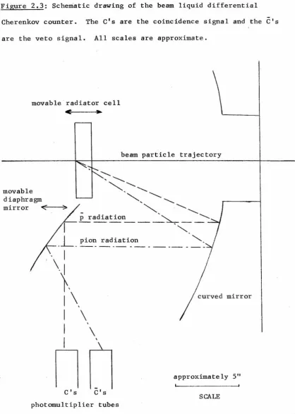
A ~.:chematic cross-sectional drawing of the liquid differential

Cl1vn~nkov counter Js shown ln Fi.gure 2.3. Tlw two 1 l.nc~s -- the

dash line and the dot-dash line, illustrate the operation of this

counter. The movable diaphragm mirror is adjusted so that Cherenkov

radiation from a p would strike the

C

bank of photomultiplier tubes

while radiation from a pion would strike the

C

bank. The difference

in radiation angle is due to the fact that pions of the same momentum

are much faster than p's and thus have a larger Cherenkov angle.

Figure 2.4a contains a plot of the proportion of coincidences

from the Cherenkov counter for each S as a function of diaphragm

mi1 . ..-01: pusU:iou ~:etting at a typical momentum. At thf.~ sc~tting

to-\vards tlw left, the pion radiation strikes C's; at the right, the

counter is sensitive only to p. The p peak is at least a factor of

20 higher than the dip between the

p

peak and the pion peak giving

evidence that much less than 5% contamination of pions underneath

the p peak is expected. Checks show that typical pion contamination

is in the 0.5% level. Efficiency for p's is better than 90% near

Figure 2.3: Schematic drawing of the beam liquid differential

Cherenkov counter. The C's are the coincidence signal and the C's

are the veto signal. All scales are approximate.

movable radiator cell

<

•

...

beam particle trajectory

movable diaphragm

mirror

*"<"---"""

'~

""-

_' ... _...

""'

'

~

...

""-

...

-

' ...

R._!adiation _ _ _ -~ _ _ -...

""'

l_

pion radiation

""'-.

-' I

\1

},

I\.

I \

I

I

n

C's

\

e's

photomultiplier tubes

curved mirror

approximately 5"

[image:26.565.63.481.81.668.2]

lOOi

100

%

r

50

i

(a)

I

I

(b)

/ \ \

_ _

1

ns

clip on

s

3

~

50

%

~

I

;

.

\ ---

----

O

ns

clip on

s

3

I

\

\ - 1

ns

clip

on

s

3

,_,

I

Ill

:

,_,

6b

_I

and

Cherenkov

co

c:

·rl

'

vetoing pions

Of.) t/l

I ·rl

t/l QJ

u

QJ

c:

I

u QJ

c: 10%

l

i

"O

QJ •rl

10

%

"-.../

I

"O u I ..

--

..

•rl c:

pions

'

' '

u •rl

'

'

c:

0 '

'

•rl

pions

p's

u • I

0 I _' !

u

5%

..c:

.IJ

5

%

I

-1

to""

~ Of.)

:

I

00

0 •rl

:

I

I

~

,_,

.

I I ' . _I

c:

1.14 I

/

I

I

I

QJ I

'

H 1.14 I

.

QJ 0

. .

I

I

' ... '

.

..c:

I

.

u QJ

p's

I

s

I

I

Of.) •rl

2nsec

c:

.IJ I

·rl

I

' I

~ Of.)

·rl

c:

Of.)

1

%

·rl

1

%

I

.

~ '

'

<::'<- •rl Of.)

J

--*

Beam Cherenkov counter diaphragm

Beam

time-of-flight delay between

s

3

and

mirror position setting

the M

1

to

M

7

counters

Figure 2.4: (a)

%

of

Cherenkov

coinci

den

ce vs.

diaphragm mirror

pos

i

tion

.

If

,

in the Figure

2.3,

the

diaphragm

mirror

moves to

the

left, the C's

wo

uld

then receive the pion radiation.

(b)

%

of beam

t

[image:27.737.64.678.62.418.2]

The liquid differential Cherenkov counter is adequate in

identifying p's and rejecting pions above 1.0 GeV/c. However, below 1.0 GeV/c, the efficiency in counting p's deteriorates. Thus, we use the Cherenkov counter to count (and reject) pions along with using a

time-of-flight system described below.

2. Beam Time-of-Flight System

A set of 7 counters(2•13)(called the mass slit counters since

they are placed next to the mass slit in the beam transport system -see Figure 2.1) about 14' upstream of the target is used in

con-junction with the

s

3 counter to give us a time-of-flight measurement

of the velocity of the beam particles. Below 1.0 GeV/c, the p has a

~ of about 0.7 while the pion has a ~ of about 1.0. Thus, the

difference in time-of-flight is about 4 nsec. Figure 2.4b shows the response as a function of time delay. The solid and dotted lines are

the response for the time-of-flight system alone while the dashed

line is the combined response of the time-of-flight with the Cherenkov

counter set to reject pions. Again, we see that the pion background

undeineath the ~ peak is reduced to the 1% level. Notice that we

clip the

s

3 signal with a 1 nsec cable to give us a broader peak. Reduction of Spurious Tracks in the wsc

We use a pile-up system to reduce spurious tracks in those

events which we record. The beam halo counter A (see Figure 2.2)

u

is situated next to

s

2 and the two counters count all the particles in

the beam. When either of these counters register a count, a pile-up

amount of usable beam by 10-20%, cannot however, entirely cure the

multiple track problem since the trigger system takes about 300 nsec

to fire the wsc. Any particle which arrives between the.backward

elastic event and the firing of the chamber will be recorded along with the backward elastic event.

To help us decide which track belongs with the backward elastic event, two arrays of 4 211 _{by 2" wide and 1/4" thick scintillation} counters called the beam hodoscopes are arranged in horizontal and vertical rows. The signals from these counters are used in the analysis. Any track which extrapolates into a counter which did not

fire is removed in case of multiple tracks. This procedure is

necessary only for a small percentage (of order of 1%) of all events.

Scaler Counting System

Our wsc impose a dead time of 20 msec each time. they are . d(2.14)

triggere • All p's satisfying our aperture and pile-up criteria

which arrive during the time in which we are sensitive to backward

elastic events must be counted. We use a series of logic modules (Chronetics 100 series -- 100

megacycl~s(

2

.lS))

and scalers to count p's. In addition, several other beam quantities such as S (the beam ·

particles, not necessarily p's, satisfying aperture and pile-up criteria) are also counted in order to monitor beam quality.

Table 2.2 lists the momenta where data were taken, the total p

flux at each momentum, typical S and

p

per pulse, pi/p ratio and

trigger rate. Figure 2.5 shows the distribution of momentum, positions and directions of the incident p's at three typical

mo-(2.16) . d h

Table 2.2: Beam fluxes and rates for each momentum •. The "Real" mo-mentum is the actual average momo-mentum at the center of the target. The

• 1 1 d t b 1 5 1012 • 1 • I

rates per typ1ca pu se correspon s o a out • x c1rcu at1ng p s

in the AGS. Runs labeled L are special runs with low bending magnet setting. Trigger rates are usually higher for these runs. In our final results, the data at 1.585 and 2.125 which has been marked with an *were combined to form the 1.59 and 2.155 data.

Momentum Nominal Real

(GeV /c) (GeV /c)

0.68

o.

77 0.89 0.92 0.97 1.09 1.34 1.45 l.585AH* l .585AL*

o.

703

0.812 0.873 0.935 0.987 1.115 1.338 1.447 1.580 1.580 1. 585BH* 1. 589 l.585BL* 1.589 l.585C* 1.596 1. 585D 1. 610 1. 70 1.815 1.8 2.0 2. 125H*

*

2 .125L

2.365 1. 716 1. 797 1.844 2.032 2.155 2.155 2.370

Total

p

flux (empty) full in millions

s

p

pi/p

per typical pulse

( 3.0)

( 6. 2) ( 4.2) (11.0)

( 7.5) ( 3.0)

( 7. O)

(10.0) (10.5) 7.0 9.1 20.0 9.5 54.2 29.8 38.8 43.0 24.5 15 .8

8K 20K 13K 33K 46K 26K 24K 24K 32K 32K 0.5K 0.9K LOK 2.5K 3.5K 4.0K 8.0K 8.5K 11.0K 11.0K 15 .0 21.0 12.0 12.0 12.0 5.5 1.9 1.8 1.8 1.8 10.8 40K 16.0K 1.5 4.4 40K 16.0K 1.5 7.9 26K 12.0K 1.1 63.3 30K 11.0K 1.8 78.2

60.3 73. 7 73,5 59.8

21. 7 48.4

35K 13.0K 1.8 55K 22.0K 1.5 40K 15 .OK 1.6 55K 22.0K

55K 28.0K

55K 28.0K 75K 45.0K

1.5 1.0 1.0 0.6

Trigger rate per 1000 p's

[image:30.568.63.476.248.676.2]

Momentum distri-

20%

bution (in units

of

1%)

40%

Horizontal position

distribution (in

30%

units of 1 cm)

20%

1::1

J

I

s

=1=1

'.:J

J

I

L

I

Vertical position

distribution

(in units of 1 cm)

30%

20

%

10

%

.

I

Figure 2.5: Distribution of momentum, positions and slopes of the incident p beam

I

I

1

I [image:31.735.46.642.47.459.2]

Figure 2.5: (continuation)

Horizontal Slope

Distribution (in

units of

10

mr)

Vertical Slope

Orfo

30

%

20%

10%

0%1

c='

I

'=,

e=1

I

I d

k

I

40'f,

i

Distribution

30%

'

(in units of

10

mr)

20%

10%

0%1 I I ~ 1

N

[image:32.739.46.644.95.520.2]

wsc resolution and multiple scattering in addition to the intrinsic properties of the beam<2•17).

Typically, we accept a momentum bite of ±

3'fo

and keep the mass slit spacing narrow (about 1/8"). The total number of beam particles as measured by Au and

s

2 per pulse is about 150 K. Since the beam pulse period is about 400 msec, this corresponds to a 0.3 megacycle rate. We have checked that this rate is tolerable since several data runs at a lower rate give answers which agree with the answer at the typical rate.

(b-ii) Target ( 2.18)

We use a cylindrical liquid hydrogen target 14-5/811 _{(37 .2 cm)}

long and 3" (7.6 cm) in diameter. The target envelope is a single jacket of 14 mil mylar surrounded by 40 layers of 0.3 mil aluminized mylar acting as superinsulation. The target, shown in Figure 2.2,

is housed in a vacuum box 15-3/4" wide set at 45° to the beam line. The liquid hydrogen in the target is maintained at atmospheric

pressure near the boiling point and has a density of 0.0708 gm/cm3

<

2•19).

(b-iii) Magnet and Momentum Measurement The magnet

n

4 we use for momentum analysis is a 48D48 dipole magnet with an aperture 18" high by 48" wide. The useful aperture, however, is restricted by the hole in the magnet shielding which is

14" x 28" upstream and 16-1/4" x 46-1/411 _{downstream of the magnet.}

. (2.20)

The shielding, an iron-wood sandwich which contains iron

layers of thickness 3/4", l", and 6" is attached to either side of the magnet by long bolts and brackets. Its purpose is to minimize the stray field outside the gap of the magnet.

High stray fields would incapacitate both the magnetostrictive

readouts of the wire spark chambers and the photomultiplier tube

(even with shielding around it). Studies have shown that the magneto-strictive wire will not function with high transverse fields (of the order of 50 gauss) although longitudinal fields of up to several

hundred gauss can be tolerated. Since the field inside the gap goes as high as 15 Kgauss, stray fields of 1% of the central field cannot

be tolerated. In addition, the photomultiplier tubes, even with

shielding, cannot withstand hundreds of gauss. Without any magnet shielding, the field at the beam line 50" from the side of the magnet is still about 1% of the field at the center of the magnet (i.e.,

about 100 gauss); the shielding reduces the field so that at the beam line 25" from the side of the magnet (just outside the shielding),

the field is reduced to about 0.1% of the field at the center of magnet gap. Even then, the wire chamber readout wires of chambers

9-12 (downstream of the magnet) must undergo special treatment when-ever we switch the polarity of the magnet (the wire must be

re-magnetized and the pick-up amplifier must have its polarity switched

also) •

The momentum of the particle which goes through the magnet is obtained from the amount of bending obtained while traversing the

obtained through the use of a nuclear magnetic resonance prohe<2·21).

We then use the rectangle field approximation to calculate the

mo-mentum.

For a particular field B at the center of the magnet, we

nppro::d.matc the field by .:i vertical field B over a length T., the

(

'

rre

c

Liv

l

~

l.engtli wbicli has beeu cmpiri.ca.1 ly delenn.i.ned to be(2•22)

L 155.60 cm/(l

+

(B/255.51 Kg)0•99991).

The momentum of the particle traversing the magnet is then

p 2.9978 B L(l

+

x

12

+

_y 12₎1_/2

. . 2 1/2

lOO(sin

a+

sin ~)(l + x' )

where x' and y' are the incident horizontal and vertical slope,

a

is the incident horizontal angle and ~ is the outgoing horizontal

angle (see Figure 2.6a). Studies have shown that this formula is

. . , /2.22)

accurnl:f'. to within O.J1

1, • Figure 2. 6 shows some of the

geom-<.:!try Pl Llie r«•(·tangl!~ l'i.e l.d approximation.

We can thus obtain the momentum of a particle at the magnet.

To obtain the momentum at the interaction vertex, we simply correct

for ionization losses.

In order to select backward elastic events using kinematics,

we must have a good idea of the momentum of the incident p. We

calibrate the incident momentum by triggering on every p and changing

the polarity of the magnet to bend negative instead of positive

p:-irticl.es into the wsc downstream of the magnet. We do this

mo-1111'11111111 c;rl i.b1-;11 ion ror t•acli of Olff moment:a. The resultant c.listr.

'I--L

IL

_.s;;

z

I

I I I I

P\ . :'/ /

\ I /p

\ \

\a I

~

/

;-N /

I I I

,..-.e,

!•=sin (a) _p

\!

_I/

y

>,v_

22

-~

2

=sin

_(,8)

e,

+ 22 L

- -_p = -_p =sin (a)+ sin (p)

...

along magnets center llne B = By only

8x

2.9978

P

=cos (a) - cos

(/J'J

where p = p 8₀ Relation Between The Horizontal Deflection of o Track And

Its Momentum (a)

Fi

gu

r

e

2

.

4)

,...

m

,...

m

CD

J

By dz= 8₀ L₈ -CD

L

2

0

L

2

z-Rectangular Field A ppraximation

---Le--~ I L

2

I 0 ( b) I L

2

z-Re

ct

a

n

g

ul

a

r

fie

ld m

odel

for a dipole m

ag

n

e

t.

N

It is possible to obtain a better estimate of the incident momentum by using the property of the beam transport system.

Appendix A, which handles the beam transport system, indicates that at the mass slit, the horizontal (x) position of the beam is strongly correlated with the momentum -- particles with momentum higher than mean momentum tend to have positive x at the mass slit (see Figure A.l of the Appendix A).

A set of 7-1/2" wide scintillation counters is placed vertically h 1. (2. 13)

next to t e mass s it • The momentum distribution of p's hitting each mass slit counter is shown in Figure 2.7a. By com-bining the 7 distributions correcting for the shift in central mo-mentum, we obtain a total distribution of Figure 2.7c instead of 2.7b for the same p's. Since the momentum spread in the distribution is also due to multiple scattering and the wire spark chamber reso-1 ution . (2.23) , t e improvement in momentum etermination is actua h . . d . . . 11 y better than indicated. In any case, the FWHM is reduced from about

1. 7% to about 1.0%.

c. Fast Counters and Logic (c-i) Introduction

During each beam pulse, thousands of p's are incident on the

(2.24)

target. We can record a maximum of 15 triggered events • Also

I

each time We trigger, the WSC (wire Spark chambers) require ·a 20 msec dead time to allow us to record the event and to allow the wsc to recover. Thus, without losing any acceptable backward elastic events, we would like to trigger on as few events as possible. We use a

(a) _(b)

M3

(c)

-1%

oc;i

+1%

+2

%

+3

%

-1%

O<fo

+1%

+2

%

+3%

Figure 2.7: Momentum distributions of

in~ident

p's at

~.O

GeV/c nominal momentum for: (a) p's

h

itting

a particular mass slit counter.

(b) all p's.

(c) all p's corrected according to which mass slit

counter it hits.

N

[image:38.735.108.668.67.453.2]

(2.25)

modules to test for the trigger condition. We are able to reduce the t r iggering to about 1 per 1000 incident p's. No

back-ward elasti.c events are Jost except for dead time . We will cJjscuss

the t r igger condition, logic and rates in Section (c-ii).

Counter :information i.s useful for analysis. For example, lhc

kiHl\vlcd~~<' of which counter registers a count (or a particul~ir eV<'.nl: may be helpful in removing a spurious track. We record

48

binary bits for each triggered event. 35 of these bits which contain the

counter and various 'coincidence information are discussed in

Sect ion (c-iii).

The other 13 bits contain in format ion on the velocity of the

forward particle essential to remove pion background underneath our

recoil protons. This includes the information from the gas thresh-old Clwn'nkov counter (Section c-iv)) and a forward outgoing p;11"t. ic I,, L inw-of-f:l i.ght systt.!m (Section (c-v)).

(c-ii) Trigger Counters, Logic and Rates

Logic

We test for the trigger condition using a system of scintilla-tion counters (listed under "non-beam counters" in Table 2.3 with their sizes and positions) and logic modules

<

2•25).

To satisfy our trigger condition, we require a coincidence of:

1. An incident p. This is determined by the

p

identification system

described in Section (b-i).

2. A forward outgoing positive particle with momentum close to that of the incident

p

and whose trajectory passes through the wsc (wire

Table

2.3:

Non-Beam Scintillation Counter Sizes and Positions

Counter

Si

ze

Position

Name

x

:l

z

x

Y..

z

(thickness)

pl

3"

7"

1/8"

-

4"

to -

l"

-

3-1/2" to 3-1/2"

38-1/4"

p2

same

-

1-1/2''

to

1-1/2"

same

same

p3

same

l"

to

4"

same

same

p4

same

3-1/2" to

\

6-1/2"

same

same

PS

same

6"

to

9"

same

same

p6

same

8-1/2" to 11-1/2"

same

same

RO

14"

24"

1/2"

-

30"

to -16"

- 12-1/4" to 11-3/4"

175-3/8"

w I-'

Rl

same

- 24-1/2" to

-10-1/2"

same

same

R2

same

- 14"

to

O"

same

same

R3

same

-

4"

to 10"

same

same

Ql

same

7"

to

21"

same

same

Q2

same

16-1/2"

to 30-1/2"

same

same

Q3

same

26-1/2" to

40-1/4"

same

same

Q4

12"

22"

1/4"

9"

to 21

"

- 11"

to 11

11

139-1/4"

Qs

same

19-1/2" to 31-1/2"

same

same

T.(i

=

1,3,5,7,9; non-overlapping)

1

5

(7-3/8") 13-1/2" 1/4"

-

28-1/4" to

8-3/8"

- 10"

to 3-1/2"

182-5

/

8"

T

.

(j =

2,4,6,8, 10; non-overlapping)

J ·.

[image:40.746.70.617.71.496.2]

counter hodoscopes P, R and T (see Figure 2. 2, page 1.2). The P R

combination is used to restrict the momentum acceptance of the

forward particle. Figure 2.8 gives a plot of the horizontal position

at the P counter plane (xp) vs. the horizontal position at the R

counter plane (xR) for all particle trajectories. The area inside the

solid line satisfies the triggering criterion in P and R. Dashed

lines drawn in Figure 2.8 show the locus of points with the same

momentum p corning from the center of the target.

T counters are required for triggering. This is used to

reduce the aperture for triggering as well as to provide an

addi-tional coincidence requirement to reduce accidentals. Note that the

T counters are also used for forward outgoing particle

time-of-flight system.

3. An absence of a nega·tive charged forward particle with esse

n-tially the incident beam momenttnn and slope. This is tested by a

combination of P Q counters. This beam veto reduces the trigger

rate by a substantial amount. Many mechanisms can be responsible for

the large amount of incident

p

which satisfy condition 2 and yet

have a forward negative charged particle with fairly high momentum.

Two such mechanisms are a) pp annihilation into ~ulti-pions in which

one (or more) positive and one negative pion goes forward, and b) pp

into pnn+ in which the momentum transfer to the p is small.

We have studied the possibility that a real backward elastic

event is vetoed by this condition. Since the final state p will

probably annihilate in the target, a forward pi minus giving a beam

33

-Figure 2.8: Triggering "area" in P-R space. x is the horizontal po-p

sition of the trajectory in the plane of the P counters. xR is the corresponding position in the plane of the R counters. Values of x

p and xR inside this "area" implies that the event satisfies the P-R counter criterion for triggering. Lines show the loci of events from the center of the target with specified momentum.

xR in inches

-10

-20

x in p inches

//

.Q,.

2

//

.Q,.

10

Triggering area of P-R criterion

[image:42.571.71.469.203.661.2]

-(see Section (d) in Chapter III).

Electronics

The trigger electronic logic system consists of a numbl•r of

fast (100 megacycles) logic modules<2·25) used to identify, with a

resolving time of about 10 nsec, the trigger condition. It also sends

the trigger signal to the wsc pulsing system, the computer interface,

and the master gate to generate a dead time during which the p

counting system and trigger logic modules are inactivated. See

section (d-iv) for further details on the operation of our recording

system after the arrival of a trigger logic signal.

The logic of the trigger system is shown in Figure 2.9.

Counter signals from the photomultipliers are shaped into standard

pulses by discriminators (Chronetics 104(2•25)). These pulses are

correlated to see if the trigger condition is satisfied. The modules

with an x in the upper right-hand corner are those modules which are

gated off by the master gate during the dead time. It is easy to see

that without these particular modules, no

p

can be counted and thus

no further trigger can be accepted.

Rates

The rates for triggering at each momentum is shown in Table 2.2.

It is about one trigger per thousand incident p.

Even though the trigger rate is only about 0.1~, the number of

events which satisfy the trigger condition is still rather large since

the average flux of p per pulse is as high as 45K. At incident

mo-mentum of 1.5 GeV/c or higher, this rate is intolerable. If w~

Figure 2.9: The trigger logic flow chart (modules which are gated off by the master gate are shown with an x in the upper right-hand corner; veto enters through the Side).

]t---<1~-!--t----'

<11

low momentum high momenttnn

ffi-1

i :

I

[image:44.572.65.484.117.677.2]

time. Since each beam pulse lasts only about 400 msec, we are only able to use

1/3

of the beam! It would be useful to reduce the trigger rate further since the actual number of backward elastic events is only about

1

%

of all the triggered events.

Several possibilities can be considered:

1. The (PR) triggering area (see Figure 2.8) can be reduced. We can use fewer combinations of P and R counters in our trigger. This would narrow our momenttnn acceptance. Due to the finite size of the

target and counters, the maximum reduction possible without losing any backward elastic events is less than

1/3.

2. We could use the gas Cherenkov counter (see Section (c-iv)) to veto all events which give a pulse since recoil protons are below threshold f6r this counter. However, the reduction is only

15

%

.

Most of the triggers are apparently due to low momentum protons or

pions below the threshold for the Cherenkov counter.

Thus, it is possible to reduce the trigger rate by about 40%. W e d . d i no t d o it since . . th e gain is . . not too s1gni . . ficant .

<

2 • 26 ) an d a so 1

since we are interested in measuring pp going into pi

+ missing

mass,

K

+

.

.

.

.

.

(2.27)

. missing mass or p

+

missing mass •

Another possible way to reduce trigger rate is to use the time-of-flight system. However, at high momentum, our system is not good enough to separate forward pious from forward protons.

(c-iii) "Counter Bits"(Z.ZS) __ Scintillation Counter Information for Analysis

- 37

-analysis and in the efficiency calculation of the counters. We cover these uses in the appropriate section in the analysis chapter.

35 of the 48 available bits record the information of whether one or a combination of counters fired. The remaining 13 bits record the information from the gas Cherenkov counter and the forward out-going particle time-of-flight system (see the next two sections).

Briefly, the co.unter bits work as follows. Counter signals are delayed and timed to arrive at the counter bit modules just after they receive the interface signal after each trigger (seed-iv). The counter bit modules remain receptive for a duration of 50 nsec. The arrival of a counter signal during this period will flip the module. The modules are then read by the interface and the

informa-tion is written onto magnetic tape. The modules are then reset to await the arrival of the next triggered event.

(c-iv)

forward

The Gas Threshold Cherenkov Counter

One of the two systems we used to measure the velocity of the (2. 9)

assume that any time we receive a coincidence from this counter, a pion has passed. Although a high energy proton or kaon could in principle

produce a pion with sufficient momentum to trigger this counter, this

b ( 2.29)

is expected to e rare •

Figure 2.10 shows a cross-sectional view of this counter and

also demonstrates how this counter works. Note that the photomulti-plier tubes sit at the top of the counter and thus they are not in

the particle's path. Hence, we do not need to worry about Cherenkov

radiation in the quartz window of the counter or the glass windows

of the photomultipliers. Not shown in the figure are the heating

coils necessary to keep the whole counter above 40°c. This is . (2.30) necessary in order to prevent the Freon-12 from condensing •

Although the counter is a cylinder 4' in diameter, the useful

radiation distance, due to the placement of mirrors, is typically

about 25i•. A total of about 50 photons are produced. (The

Cherenkov radiation is focused by the curve-mirror and flat-mirror

system into an area covered by light pipes.) Our phototubes (2.31)

have about 10% quantum efficiency. Thus, an average of 5

photo-electrons are produced. The resultant signal from the

photomulti-pliers are mixed and fed into a 64-channel pulse height analyzer.

The output is recorded in 6 binary bits of the counter bits.

Figure 2.lla shows a typical pulse h~ight distribution for forward

particles near the incident momentum. Figure 2.llb shows the portion

of the events in 2.lla which are tagged as pi's by the time-of-flight

system discussed in the next section. The cut we usually use is

39

-Figure 2.10: Schematic drawing of the gas threshold Cherenkov counter. The dashed lines are rays of Cherenkov radiation from a particle with velocity above threshold (about 1.1 GeV/c for pions).

approx. scale

o"

s'"

10"

Light pipes

Cherenkov radiation

____

f- _

_ _

_

Cherenkov r~ation_

~--/

-

-~

---

.----

e

the Cherenkov an le

--

--

_---~-..

- - --- -- - - ----+- - -

===-mirror

tubes

Particle trajectory

[image:48.566.61.494.166.664.2]

Figure 2.11: Cherenkov pulse height channel distributions for: (a) Particles with momentum about 1.61 GeV/c

(b) Particles in distribution (a) which are tagged as pions by the time-of-flight system.

(c) Particles with momentum about 0.92 GeV/c (below threshold for Cherenkov radiation even for pions).

400

overflow

Number (a)

300

200

100

20 40 60

Cherenkov pulse height channel number

(b)

so

20

I

40 60

pedestal

pedestal cut

100

l

(c)

so

[image:49.568.49.487.140.678.2]

From 2.llb we see that we usually remove 75-85•/, of all the pi's by

throwing away all events with Cherenkov pulse height channel above

the arrow. Figure 2.llc shows a distribution of particles with

mo-mentum below threshold. We see that less than 2% of such particles

have a Cherenkov pulse height above the arrow. Thus, we expect to

lose less than 2% of protons by making this cut.

As mentioned above, the counter cannot separate about 20%

of the pions from the protons. This is not due to the design of the

counter. Although the counter was not built expressly for the

(2. 9)

experiment and the geometry is not ideal, the mirrors are

adjus-table and we can still focus the light without significant loss in

our geometry. We could have better performance by using

photo-1 . l" b i h h. h ff. .

<

2 • 32)

mu tip ier tu es w t ig er quantum e iciency . This was

re-jected due to cost. We used some available photomultiplier tubes (2.31)

which g