A convolution-deconvolution method for improved storage and communication of remotely-sensed image data

(1)

PROCEEDINGS OF SPIE

SPIEDigitalLibrary.org/conference-proceedings-of-spie

A convolution-deconvolution method

for improved storage and

communication of remotely-sensed

image data

Gabriel Scarmana, Kevin McDougall

Gabriel Scarmana, Kevin McDougall, "A convolution-deconvolution method

for improved storage and communication of remotely-sensed image data,"

Proc. SPIE 10780, Multispectral, Hyperspectral, and Ultraspectral Remote

Sensing Technology, Techniques and Applications VII, 107800Z (13

November 2018); doi: 10.1117/12.2324451

Event: SPIE Asia-Pacific Remote Sensing, 2018, Honolulu, Hawaii, United

States

(2)

CONVOLUTION-DECONVOLUTION METHOD FOR IMPROVED STORAGE AND

COMMUNICATION OF REMOTELY-SENSED IMAGE DATA

Gabriel Scarmana and Kevin McDougall School of Civil Engineering and Surveying University of Southern Queensland, AUSTRALIA

ABSTRACT

An essential feature of remote sensing and digital photogrammetric processes is image compression and communication over digital links. This paper investigates the probability of using a convolution-deconvolution method as a pre-post-processing step in standard digital image compression and restoration. As such, the paper relates to image coding and compression systems whereby an original image can be transmitted or stored in a convolved (i.e. blurred) representation which renders it more compressible. The image is then thoroughly restored to its original state by reversing the convolution process.

The compressibility of an image increases with blurring, whereby the relation between the compression ratio (CR) and the blurring scale is almost linear. Hence, by convolving by way of a localised response function (i.e. a linear kernel) and thereby blurring an image before compression, the CR will increase accordingly. In this novel process the response function is applied to a fractal one-dimensional representation of a given image. A blurred image is thus created, which can be shown to contain the details of the original image and thereby restored by reversing the blurring process. The implications of increased CR are examined in terms of the quality of the reconstructed images.

Keywords: Image compression, Image convolution, Image deconvolution, Image restoration.

1. INTRODUCTION

The objective of image compression is to reduce irrelevance and redundancy of the image data in order to be able to efficiently store and/or transmit data. Image compression may be lossy or lossless. Lossless and lossy compression protocols are well explained in the related literature and the reader is referred to [1] [7] and [8] for a thorough definition and application of image compression systems.

It is worth saying that very few processes have considered convolving an image (e.g. blurring) or using the convolved or blurred image to provide compressed data. It has not therefore been appreciated that the blurred image contains all the detail of the original and that the blurring function provides the key or code by means of which the original can be restored from the blurred version without significant loss of pixel brightness resolution.

Hence, blurred images can be compressed much more efficiently than images with a lot of (high-frequency) details. This is because sharp details in an image normally produce many high-frequency components, and therefore many significant bits are required for a correct representation of an image, which all have to be encoded.

In the spatial domain blurring can be achieved using pixel-group operations or more specifically using neighbourhood operators. Neighbourhood operators basically combine a small area or neighbourhood of pixels to generate an output pixel. The most important neighbourhood operator is convolution, and at the heart of this operation is the convolution mask or kernel [12][9].

Convolution requires a lot of computational power. To calculate a pixel for a given mask of size m x n, m * n multiplications, m * n - 1 additions, and one division are required. So to perform a 3 x 3 convolution on a 1024 x 1024 colour image (a minimal convolution on an average-size image), 27 million multiplications, 24 million additions, and 3 million divisions are performed. For more substantial convolutions, such as 5 x 5 or 8 x 8, on larger images the amount of computation required is indeed very large. Some of the most common applications that use convolution are digital filters. Common digital used to achieve blurring are [10]:

(1) Mean or average filter (2) Weighted average filter and (3) Gaussian filter

Multispectral, Hyperspectral, and Ultraspectral Remote Sensing Technology, Techniques and Applications VII, edited by Allen M. Larar, Makoto Suzuki, Jianyu Wang, Proc. of SPIE Vol. 10780, 107800Z

(3)

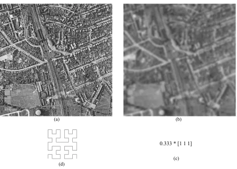
To illustrate the effect of blurring in terms of achievable image compression, the reader is referred to Figure 1 which shows an 8 bits grey-scale image called aerialview.BMP (12002_{pixels) and its blurred version. The blurred version of}

aerialview.BMP was accomplished by firstly representing this image in one-dimension by way of a well know fractal curve referred to as the Hilbert space filling curve. The Hilbert space filling curve has been considered for numerous image processing applications [11][2]. It is primarily used as it has a strong locality property as it never leaves its current quadrant, at any level of image representation, before traversing all the pixels of the quadrant. In this example, the Hilbert curve was used to allocate each newly created pixel in the correct order and location when displaying the blurred image in 2D.

(a) (b)

[image:3.612.64.543.172.513.2]

(c) (d)

Figure 1 - Original 8 bits grey-scale image (12002_{pixels) of aerialview.BMP (a), and a blurred version (b) using a one-dimensional}

spatial low-pass filter (i.e. box filter) (c) iteratively 4 times. The fractal space filling curve (Hilbert curve) used to transform the aerialview into a 1D representation is in (d).

Accordingly, a one-dimensional low-pass average (or box) filter consisting of a kernel (or mask) of 1x3 pixels was used iteratively four times so as to emulate the effect of a Gaussian filter [8]. Note that a single pass with a larger kernel would have produced a similar but not identical effect as a single pass with a larger kernel. Smaller kernels however, have a favourable effect on processing edges in an image.

The memory requirement to save the image aerialview.BMP uncompressed was 1.2 megabytes. To save the same image as a .BMP RLE (Run Length Encoding) compressed file did not have a significant impact on the CR. On the other hand, the same image stored as a .PNG (Portable Network Graphics) or as a lossless .J2K (JPEG2000) required approximately 0.6 and 0.7 megabytes respectively for a relative CR of 2.7 and 1.9. The blurred version needed approximately 0.3 megabytes for its storage as a .PNG and 0.37 as a lossless .J2K file for a respective CR of 4.7 and 4.02.

As mentioned earlier and as illustrated in Figure 1, blurring causes a radical restructuring of the data in the spatial transform domain, greatly increasing amplitudes at low frequencies relative to high frequencies. Hence, for blurring to be

0.333 * [1 1 1]

Proc. of SPIE Vol. 10780 107800Z-2

(4)

considered as a compression tool it should provide the capability of integrally restoring or de-blurring the blurred image. Generally, blurring can be de-blurred and there exist many deblurring algorithms and processes in the literature.

Examples of image deblurring with applications and inherent variation models can be readily found in specialised image processing software such as www.mathwowrks.com (see the Matlab image processing tool). Examples and relative variations of these techniques are [3]:

(1) Blind deconvolution; (2) Lucy-Richardson method; (3) Regularized filter and (4) Wiener filter.

On the other hand, the observed blurred image only provides a limited constraint on the solution and with no additional constraints, there are many blur kernels or distortion operators or point spread function (PSF) which may define the degree to which an optical system blurs (spreads) a point of light and images that can be convolved together to match the observed blurred image. Even if the blur process is known, there still could be many sharp images that when convolved with the blur kernel can match the observed blurred and noisy image [6].

One of the central challenges in image deblurring is to develop deconvolution methods that can discriminate between several potential solutions and delineate a deconvolution or deblurring process toward more likely outcomes given some prior information. In this context, this work provides an alternative technique for creating a blurred image which can be stored or transmitted as a compressed representation of the original image, without sacrificing the detail of the original image, even though the blurred image appears degraded to a point that the original is not identifiable from the blurred version.

Moreover, the primary object of this research is to provide an improved system for convolving and compressing an image, and particularly, data representing that image whereby high compression ratios can be obtained and the original image accurately recovered from the blurred and compressed representation.

Also, the proposed technique provides an enhanced system whereby image data may be programmed into a compressed form so as to offer compression ratios which can be controlled by varying the same encoding function. The image can then be accurately decoded or deconvolved only with knowledge of the initial blurring function which can be readily changed from time to time so as to suit different security or personal requests.

The previously mentioned and other objects of this work, as well as the mathematics and/or mechanics behind the proposed process, will become more apparent from the ensuing description.

2. THE CONVOLUTION-DECONVOLUTION PROCESS

Consider an initial Image X, comprising a line of 9 pixels (Xi) as shown below, and representing a high frequency signal to be blurred (i.e. convolved) and thereafter integrally restored (de-convolved).

Image X

189 35 78 250 10 100 150 30 230

Image C

75 101 121 113 120 87 93 137 87

The blurring effect is such that each generated pixel Cn (n=1-9) of the convolved Image C is the result of convolving

Image X by applying the 1x3 kernel [0.333 0.333 0.333] in figure 1(c). Generating image C required Image X to be convolved at a rate so that Image C can adequately resolve all the spatial details of the original continuous-tone image (Image X). This guarantees that the deconvolution process will restore the original Image X in all its details.

(5)

This was accomplished in line with the classic sampling theorem [3]. This theorem implies mathematically that in order to represent fully the spatial details of an original continuous-tone image, it is required to sample the image at a rate at least twice as fast as the highest spatial frequency contained in it. This means that to capture an image's finest dark-to-light-to-dark detail, sampling must take place at a rate that at least two samples fall upon the detail. This guarantees that both the dark and light portion of the detail are sampled, and hence preserved, in the resulting digital image.

Accordingly, the pixels of Image C are calculated as per the following nine linear relationships:

C1= (X1+X2+0)*0.333 = 75

C2 = (X1+X2+X3)*0.333 = 101

C3 = (X2+X3+X4)*0.333 = 121

C4 = (X3+X4+X5)*0.333 = 113

C5 = (X4+X5+X6)*0.333 = 120

C6 = (X5+X6+X7)*0.333 = 86

C7= (X6+X7+X8)*0.333 = 93

C8 = (X7+X8+X9)*0.333 = 137

C9 = (X8+X9+0)*0.333 = 87

By knowing the values of the Cn and the equations used for their estimates it is possible to restore the original pixels

Xi. The set-up shown below is simply a rearrangement of the above equations in matrix form [4]. The required

coefficients (Cn) to solve and obtain the original pixels Xi are given on the right hand side.

Note that in order to restore the original values of Image X the results from solving the system of equations must be multiplied by 3. Also, since the pixels of Image C are rounded to the nearest integer an exact restoration of Image X may not always be achieved. In this simplistic linear example the RMSE of the differences between the original Image X and the restored one was +/- 0.3 intensity values.

The above convolution-deconvolution process was programmed in Matlab R14 (www.Mathworks.com) so as to be applicable to grey-scale images of any size. As mentioned earlier, the process may readily be changed so as to suit different security, corporate and/or personal requirements.

A number of tests were carried out with images containing various degrees of high/low frequency details (i.e. entropies). A detailed example is given in the ensuing test.

3. TESTS

Following the concepts of Section 2, the same image referred to as the aerialview (12002_{pixels) in Figure 1(a) was}

considered in this test. However, rather than using .bmp, .png and .jpeg2000 image formats, this test considered a .TIFF version of the same image. The purpose here was to demonstrate that the proposed process is applicable to all image formats.

The uncompressed aerialview.TIFF (1.3 megabytes) was divided into matrices of 8x8 pixel blocks. That is, 22500 blocks. The pixels within each block were connected or represented in one-dimension using the Hilbert fractal curve as per the diagram in Figure 1(d). This preliminary practice was implemented because attempting to apply the process detailed in the previous section as a whole to the entire image would not yield the most favourable results [5][9].

[A] = 1 1 0 0 0 0 0 0 0 1 1 1 0 0 0 0 0 0 0 1 1 1 0 0 0 0 0 0 0 1 1 1 0 0 0 0 0 0 0 1 1 1 0 0 0 0 0 0 0 1 1 1 0 0 0 0 0 0 0 1 1 1 0 0 0 0 0 0 0 1 1 1 0 0 0 0 0 0 0 1 1

[C] = 75 101 121 113 120 87 93 137 87

[Xi] = [ATA] -1* [ATC] * 3

(6)

In addition, this allowed the proposed process to take advantage of the fact that similar pixel intensity values were likely to appear together in small parts of an image. The blocks started at the upper left part of the image, and were created going towards the lower right.

The convolution of each line of 64 original pixels was achieved as per section 2. Rather than 9 pixels, however, 22500 blocks of 64 linear pixels each were convolved sequentially 2 times with the same 1x3 average filter of Figure 1(c). To store this heavily blurred image as an uncompressed .TIFF still required 1.3 megabyte. The same image was then compressed using a TIFF related lossless compression protocol (i.e. LZW) and the memory requirement for its storage was reduced to 0.48 megabytes for an overall CR of 2.8.

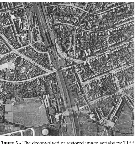
The visual outcome of deconvolving and thereby restoring aerialview.TIFF from its blurred representation is illustrated in Figure 3(a) and it required 6 seconds. That is, to solve the system of equation for 64 unknowns repeated 22500 times. This time was calculated based on the clock function of Matlab R14 on a Windows 7 Home Premium platform with a 2.10 GHz processor, a RAM of 4.0 GB and a 64-bit Operating System. Also to be noted is that the system of equations to solve for a single block of 64 pixels was replicated exactly in the same way for each of the 22500 blocks. The only variation to the system was of course the Cn coefficients which would be different for each block.

[image:6.612.194.421.286.529.2]

The restored aerial image was statistically compared with the original aerialview.TIFF by way of calculating the RMSE of the difference between the original aerialview.TIFF and the restored version. The RMSE in this case was +/- 2.75 pixel intensity values with maximum and minimum differences of -3.8 and 2.9 pixel intensity values.

Figure 3 - The deconvolved or restored image aerialview.TIFF

Also to be mentioned is that the restored image did not present major defects along the boundaries which are usually the case for standard convolution low-pass filters and or window-moving operations based on pixel group processing.

4. CONCLUSIONS AND CONSIDERATIONS

This paper provides an alternative system for data encoding and compression of digital images representing data which utilizes controlled convolution in accordance with a code that renders the original scene very blurred and degraded in the convolved or encoded image. The blurred image can be decoded or deconvolved successfully only with knowledge of the blurring function (kernel), which can readily be changed so as to suit necessary requirements.

In image deconvolution (in this case deblurring) the purpose is to restore an original image by using a mathematical model of the blurring process [9]. The key issue is that some information on the lost details is indeed present in the blurred image, but this information is “hidden” and can only be accurately recovered by knowing the details of the blurring process. The original image cannot be restored exactly due to various unavoidable errors in the encoding

(7)

process. The most relevant errors are rounding errors which are due to the integer nature of representing pixels digital images.

Further tests are required to determine the limitations and effect of other types of kernels (or filters) using in principle the same process described in this contribution. Sufficient to say that in the case of deblurring images by simply applying sharpening or high-pass filters (i.e. kernels) to a blurred image do not produce satisfactory results.

Although sharpening operations enhance features of an image, it should be mentioned that they add no information to it. It should also be implicit that although, in a sense, blurring and sharpening are opposite, they are not true inverses. That is, by blurring and image and thereafter sharpening it, or sharpening it and then blurring it, the original image will not be restored. The information then is lost and when these operations are applied they cannot be restored.

REFERENCES

[1] Bovik A. (2005). Handbook of Image and Video Processing. Academic Press. 400 pages.

[2] Bader M. (2012). Space Filling Curves: An Introduction with Applications in Scientific Computing. Springer Berlin Heidelberg. 278 pages

[3] Khorram, S., Koch, F.H.,van der Wiele, C.F., Nelson. (2012). Remote Sensing. Chapter 3. Springer-Verlag New York. 134 pages.

[4] Fryer J. and McIntosh K. (2001). Enhancement of image resolution in digital photogrammetry. PE&RS, 67(6):741-749. [5] Showengerdt R. A. (2007). Remote Sensing: Models and Methods for Image Processing. 3d Edition. Elsevier.

[6] Luhmann T., Robson S., Kyle S. and Boehm J. (2013). Close-Range Photogrammetry and 3D Imaging. De Gruyter publisher. Chapter 5 - Digital Image Processing. 684 pages.

[7] Gonzalez R. Woods R. and Eddins S. (2009).Digital Image Processing Using MATLAB, 2n edition. 827 pages. [8] Russ C. J. (2011). The Image Processing Handbook. 6th Edition, CRC Press, 885 pages.

[9] William M. Wells (1986). Efficient Synthesis of Gaussian Filters by Cascaded Uniform Filters. IEEE Transactions on Pattern Analysis and Machine Intelligence (Volume: PAMI-8, Issue: 2, March.

[10]Richards J. A. (2012). Remote Sensing Digital Image Analysis: An Introduction. Springer Science & Business Media. 494 pages.

[11]Sagan H. (1994). Space Filling Curves. Springer-Verlag New York Inc. 194 pages

[12]Wolf R., Dewitt B. and Wilkinson B. (2014). Elements of Photogrammetry with Applications in GIS. McGraw and Hill education. 676 pages.