Determining the mid-plane conditions of circumstellar discs using gas and dust modelling: a study of HD 163296

Determining the mid-plane conditions of circumstellar discs using gas and

dust modelling: a study of HD 163296

Dominika M. Boneberg,

Olja Pani´c,

†

Thomas J. Haworth,

Cathie J. Clarke

and Michiel Min

1_{Institute of Astronomy, Madingley Road, Cambridge CB3 0HA, UK}

2_{SRON Netherlands Institute for Space Research, Sorbonnelaan 2, NL-3584 CA Utrecht, the Netherlands}

3_{Astronomical Institute Anton Pannekoek, University of Amsterdam, Science Park 904, NL-1098 XH Amsterdam, the Netherlands}

Accepted 2016 May 27. Received 2016 May 27; in original form 2016 March 2

A B S T R A C T

The mass of gas in protoplanetary discs is a quantity of great interest for assessing their planet formation potential. Disc gas masses are, however, traditionally inferred from measured dust masses by applying an assumed standard gas-to-dust ratio ofg/d=100. Furthermore, measuring gas masses based on CO observations has been hindered by the effects of CO freeze-out. Here we present a novel approach to study the mid-plane gas by combining C18_O

line modelling, CO snowline observations and the spectral energy distribution and selectively study the inner tens of au where freeze-out is not relevant. We apply the modelling technique to the disc around the Herbig Ae star HD 163296 with particular focus on the regions within the CO snowline radius, measured to be at 90 au in this disc. Our models yield the mass of C18O in this inner disc region ofMC18_O(<90 au)∼2×10−8 M. We find that most of our

models yield a notably lowg/d<20, especially in the disc mid-plane (g/d<1). Our only models with a more interstellar medium (ISM)-likeg/d require C18_{O to be underabundant}

with respect to the ISM abundances and a significant depletion of sub-micron grains, which is not supported by scattered light observations. Our technique can be applied to a range of discs and opens up a possibility of measuring gas and dust masses in discs within the CO snowline location without making assumptions about the gas-to-dust ratio.

Key words: techniques: interferometric – protoplanetary discs – circumstellar matter – stars: pre-main sequence.

1 I N T R O D U C T I O N

Protoplanetary discs – discs of gas and dust that surround young pre-main-sequence stars – are the birthplaces of planets. With new observational facilities such as the Atacama Large Millime-ter/submillimeter Array (ALMA) providing data of unprecedented resolution and sensitivity, we have the opportunity to study the disc structure and through it, the processes that lead to planet forma-tion in more detail than ever before. However, interpretaforma-tion of these observations is reliant upon comparison with the expected emission properties from numerical models of discs. Protoplane-tary discs consist of gas and dust. In the interstellar medium (ISM), the mass ratio of these two components is canonically assumed to beg/d=100 as has been inferred from observations (see e.g. Fr-erking, Langer & Wilson1982; Lacy et al.1994). Due to the lack of observational constraints thereof, this value is often also adopted

_{E-mail:[email protected]}

†Royal Society Dorothy Hodgkin Fellow.

for discs. Pani´c et al. (2008) obtain a range between 25 and 100 forg/dfrom their modelling of the Herbig Ae/Be star HD 169142, depending on the dust opacity they assume, Meeus et al. (2010) narrowed down this range to∼22–50. In 51 Oph, Thi et al. (2013) find a value ofg/dconsistent with 100, the same holds true for HD 141569 (Thi et al.2014). The study by Williams & Best (2014) of several T Tauri stars yieldsg/dthat are relatively low (40; the values they obtain for a few Herbig Ae/Be stars are also rather low, with the exception of HD 163296, where they obtaing/d=170).

The gas governs the disc dynamics and motion of the dust, whereas dust provides the opacity to capture the stellar flux, re-radiate it and heat the disc. In order to understand the structure of discs, it is therefore crucial to study the spatial distribution and properties of both components (see e.g. Beckwith & Sargent1987; Dutrey, Guilloteau & Simon1994; Isella et al.2007; Pani´c et al.

2008; Qi et al.2011; Pani´c et al.2014). Planets are believed to form in the disc mid-plane and thus understanding the disc conditions in these regions is particularly important for constraining models of planet formation (see e.g. Boley & Durisen2010; Forgan & Rice

2013).

Many discs have bright emission in the millimetre (mm) con-tinuum (e.g. Beckwith et al.1990; Dutrey et al.1996; Mannings & Sargent1997; Andrews & Williams2007; Andrews et al.2009,

2010; Qi et al.2011), tracing the dust in the disc. Due to the uncer-tainties associated withg/dand the dust grain properties, inferring the disc mass from continuum measurements is, however, only a rough approximation. Therefore, molecular emission lines are used alternatively or additionally and allow the inference of spatial and temperature structure. The most abundant molecule in discs is cold H2gas, however, this is difficult to observe due to the lack of a

dipole moment and its low-transition probability. Thus, molecules such as12_CO,13_{CO and C}18_{O and their respective transitions are}

employed instead.

Abundances of molecular tracers are influenced by the condi-tions in the disc: for example, CO can be photodissociated in the disc atmosphere or frozen out in the disc below a temperature of

T≈19 K (Qi et al.2011). Recently, it has been claimed that the exact value of the freeze-out temperature can vary from disc to disc (e.g. Qi et al. (2015) model the snowline at a temperature of 17 K in TW Hya and 25 K in HD 163296) and depends on the chemical history of the ice (Garrod & Pauly 2011). Moreover, the transi-tions of the CO emission lines become optically thick at different heights within the disc, depending on the abundance of the particu-lar isotopologue (e.g. van Zadelhoff et al.2001; Dartois, Dutrey & Guilloteau2003; Miotello, Bruderer & van Dishoeck2014) and thus optical depth effects compromise the ability to obtain disc masses from the more abundant species. C18_{O is an important diagnostic}

of the unfrozen part of the disc mass, being much less abundant than other CO species ([16_O]/[18_{O]=557±30; Wilson1999). Its}

transitions in the mm wavelength regime are mostly optically thin throughout the whole disc and thus provide an excellent probe of the disc mid-plane. This is evidently of great importance since most of the gas mass resides near the disc mid-plane and it is here that planets are expected to form. However, only a handful of observa-tions of C18_{O exist so far, including AB Aurigae (Semenov et al.} 2005), HD 169142 (Pani´c et al.2008), MWC480 (Akiyama et al.

2013), HD 142527 (Perez et al.2015) and HD 163296 (Qi et al.

2011; Rosenfeld et al.2013). There are also C18_{O data available on}

several T Tauri stars studied by Williams & Best (2014). Further-more, there exist observations of C18_{O in TW Hya, V4046 Sgr, DM}

Tau, GG Tau and IM Lup (see Williams & Best2014, and references therein).

The CO snowline radius is the location in the disc mid-plane at which CO condenses from the gas phase and freezes out on to dust grains. This radius can be observed as a steep decline in the C18_O

density or by the presence of other molecular tracers such as N2H+

and DCO+(Qi et al.2011; Mathews et al.2013; Qi, ¨Oberg & Wilner

2013b; Qi et al.2015; Carney et al., in preparation). However, the formation path of DCO+is not fully understood and this molecule does not probe the disc mid-plane but the entire surface of the 19– 21 K isotherms. Hence, Qi et al. (2015) find that DCO+ is not a reliable tracer of the CO snowline location. They employ ALMA N2H+J = 3–2 observations instead that originate predominantly

from the mid-plane and are therefore more reliable. The presence of gas-phase CO slows down the formation of N2H+and

acceler-ates its destruction. Thus, gas-phase N2H+exists in regions where

CO is depleted, so the N2H+emission will be distributed in a ring

whose inner radius marks the CO snowline location. Therefore, Qi et al. (2015) propose that observations of C18_{O and N}

2H+are very

powerful as they directly probe the temperature of the disc mid-plane. This is important for calculations of the vertical hydrostatic equilibrium in discs which crucially depend on the conditions in

this disc region. However, the exact freeze-out temperature of CO is not known unambiguously, depends on the conditions of the en-vironment and is assumed to be between∼17 K (Qi et al.2013a, in TW Hya) and∼30 K (Jørgensen et al.2015, in an embedded proto-star). Also, the composition of the ice will influence the freeze-out temperature (∼20 K for pure CO ice,∼30 K for mixed CO-H2O ice;

Collings et al. (2004)). In addition, the gas pressure can also have an impact on the freeze-out temperature (Fray & Schmitt2009); however, Stammler et al. (in preparation) find that changes in the gas pressure in the disc mid-plane are not sufficient to shift the CO snowline radius by amounts which would cause an observable effect in our observations. Nevertheless, measurements of the snow-line location are important as they give constraints on the mid-plane temperature profiles of discs.

Another important tool for studying protoplanetary discs is the spectral energy distribution (SED) that combines independent mea-surements in a range of wavelength regimes that trace different parts of the disc (see e.g. Boss & Yorke1996; Dullemond2002; Meijer et al.2008, Pani´c et al., submitted, for studies of the influ-ence of disc parameters on the resulting SED). As the dust content of the disc influences its opacity and thus determines how much stellar flux can be intercepted and re-radiated by the disc, the SED crucially depends on the properties and vertical distribution of dust. Thus, a combination of C18_{O observations, additional data on the}

CO snowline radius and the SED provide a powerful combination of observables to model protoplanetary discs, combining independent measurements of both gas and dust.

In this paper, we model the disc around the 2.3 M(Qi et al.

2011) Herbig Ae star HD 163296, that is assumed to have an age of∼5 Myr (Natta et al.2004). It is situated at a distance of aboutd

=122 pc (van den Ancker, de Winter & Tjin A Djie1998) with a luminosity ofL=37.7 Land an effective temperature ofTeff=

9250 K (Tilling et al.2012). We list the observational properties of both the star and disc in Table1. Interestingly, the outer radius of the disc as inferred from CO emission studies (Qi et al.2011; de Gregorio-Monsalvo et al.2013) and scattered light (Grady et al.

2000) is about double the value of the disc outer radius observed in the continuum (de Gregorio-Monsalvo et al.2013). It is worth noting that HD 163296 is a relatively bright Herbig Ae star (L_∗=

37.7 L; Tilling et al.2012), thus, its disc is comparatively warm and its C18_{O line emission strong. Furthermore, the disc is observed}

to have a gap in polarized light atRgap∼70 au (Garufi et al.2014).

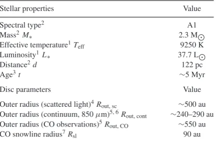
Table 1. Observational stellar and disc properties of HD 163296 from:1Tilling et al. (2012),2Qi et al. (2011),3Natta et al. (2004), 4_{Grady et al. (2000),}5_{de Gregorio-Monsalvo et al. (2013),}6_Guidi et al. (2016) and7_{Qi et al. (2015). We use a Kurucz model for the} star.

Stellar properties Value

Spectral type2 _A1

Mass2_M

∗ 2.3 M

Effective temperature1_{Teff 9250 K}

Luminosity1_L

∗ 37.7 L

Distance2_{d 122 pc}

Age3_{t ∼5 Myr}

Disc parameters Value

Outer radius (scattered light)4_{Rout, sc ∼500 au} Outer radius (continuum, 850μm)5, 6_{Rout, cont ∼240–290 au} Outer radius (CO observations)5_{Rout, CO ∼550 au}

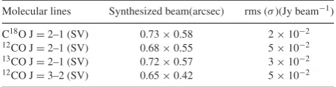
Table 2. Summary of the available ALMA observations (molecular lines in Bands 6 and 7).

Molecular lines Synthesized beam(arcsec) rms (σ)(Jy beam−1₎ C18_{O J=2–1 (SV) 0.73×0.58 2×10}−2 12_{CO J=2–1 (SV) 0.68×0.55 5×10}−2 13_{CO J=2–1 (SV) 0.72×0.57 3×10}−2 12_{CO J=3–2 (SV) 0.65×0.42 5×10}−2

Its molecular lines (mostly CO) and continuum have been studied in detail in the mm and sub-mm (Mannings & Sargent1997; Natta et al.2004; Isella et al.2007; Qi et al.2011) and recently also with ALMA (de Gregorio-Monsalvo et al.2013; Rosenfeld et al.2013; Mathews et al.2013; Flaherty et al.2015; Qi et al.2015; Guidi et al.

2016).

Rosenfeld et al. (2013), de Gregorio-Monsalvo et al. (2013) and Qi et al. (2015) employed ALMA data for modelling of the disc of HD 163296 but we are the first to use the C18_{O J=2–1 data}

to model disc parameters. Rosenfeld et al. (2013) focused mainly on modelling CO and13_{CO, whereas de Gregorio-Monsalvo et al.}

(2013) analysed the Band 7 data (12_{CO J=3–2 and continuum)}

and Guidi et al. (2016) were most interested in the dust properties and hence the continuum observations. Qi et al. (2015) also studied the C18_{O emission, but they were mostly interested in analysing}

the snowline location and comparing the C18_{O and N}

2H+emission.

In addition, Flaherty et al. (2015) used the available C18_{O data,}

but focused on the turbulence in the disc. We describe the relevant ALMA observations in the next section and stress that we base our modelling on the available ALMA C18_{O data as a crucial ingredient.}

Qi et al. (2011) had inferred a snowline radiusRsl ∼ 155 au

from13_{CO observations which was consistently also derived by}

Mathews et al. (2013) from DCO+ observations. However, more recent studies by Qi et al. (2015) find a snowline radiusRsl∼90 au

from both N2H+and C18O ALMA observations.

We do not aim to provide one best-fitting model for the disc around HD 163296, but rather want to emphasize the degeneracies in the parameters of the modelling process and propose a way to overcome them. Our main goal is to investigate the mid-plane gas temperature and density in this disc using a novel modelling approach. In Section 2, we summarize and discuss the observations. In Section 3, we describe in detail our modelling process and all the steps involved. In Section 4, we specify the models we obtain, their implications and potential degeneracies and also discuss their properties. We summarize our findings and conclusions in Section 5.

2 A L M A O B S E RVAT I O N S

2.1 Description of observations

Science verification data of HD 163296 were taken by ALMA in Band 6 and 7 (Rosenfeld et al.2013). The ALMA observations are provided as 3D fits cubes with two spatial and one spectral axis (velocity/frequency) on the ALMA Portal.1_{There is calibrated and}

cleaned data with a resolution of∼0.7 arcsec (∼85 au atd=122 pc) available for12_{CO J=2–1,}13_{CO J=2–1 and C}18_{O J=2–1 (all Band}

6), as well as for12_{CO J=3–2 (Band 7). We list the corresponding}

rms noise values and beam sizes in Table2. We use the Common Astronomy Software Applications,CASAsoftware package version

1_{https://almascience.nrao.edu/alma-data/science-verification/overview}

4.4.0 (McMullin et al.2007), to analyse the respective transitions. Amongst the transitions listed above, the C18_{O J=2–1 is relatively}

unexplored and the one on which our work focusses. We employ the already self-calibrated and cleaned Science Verification data provided on the ALMA Portal.

C18_{O J = 2–1 observations (Band 6) of HD 163296 (RA=}

17h₅₆m₂₁s_{.281, Dec.=−21}◦_{5722.36; J2000) were taken with 24} ALMA antennas (12 m) in 2012, on June 9 and 23 and July 7 with baselines spanning 20–400 m and a total on-source time of 84 min (Rosenfeld et al.2013). For a detailed summary of the spectral win-dows and calibrations, see Rosenfeld et al. (2013). The beam size of the reduced and cleaned C18_{O data is 0.73 arcsec×0.58 arcsec, the}

spectral resolution is 0.33 km s−1_{(∼0.24 MHz) with 150 channels,}

ranging from 219.571 to 219.534 GHz, where the rest frequency of the transition is 219.56 GHz. We plot the integrated emission and intensity-weighted velocity maps of C18_{O J= 2–1 in Fig.1}

and describe them in more detail in the next section. We find an integrated intensity of C18_{O J=2–1 of 6.2±0.4 Jy km s}−1_{, which}

is consistent with the values obtained by Qi et al. (2011,2015) and Rosenfeld et al. (2013).

2.2 Spatial structure of the emission

We plot the frequency-integrated intensity maps and intensity-weighted velocity maps for both transitions of12_{CO, as well as}

C18_{O and}13_{CO in Fig.1.}2_{We will focus in more detail on C}18_{O in}

this paper, but show all of these maps here as we explore the disc geometry also by using these other molecular species. Additionally, we present the continuum map of Band 6. From the extent of the disc in the panels of Fig.1, it is clear that the molecular species and the continuum trace different parts of the disc. The CO isotopes of different abundances trace down to varying depths in the disc, due to their different opacities.

Using theCASAsoftware package, we can determine the position

angle (PA) of the disc from C18_{O observations (image deconvolved}

from beam), which we find to be PA=(132.8±3.4)◦. This is in agreement with what other studies have found from CO and con-tinuum observations (Qi et al.2011; Rosenfeld et al.2013). Fitting a 2D Gaussian to the spatial profile of the emission withCASA

al-lows us to determine the inclination of the disc for the different tracers shown in Fig.1(wherei=0 corresponds to the disc be-ing face-on). From the C18_{O emission, we obtain an inclination of}

i=(47.9±1.6)◦, which is comparable to the inclination ofi=44◦ used by Qi et al. (2011). For the other molecular species, we per-formed the same analysis and obtained the values given in Table3. The value we find for the PA from the12_{CO J=3–2 is comparable}

with the one from de Gregorio-Monsalvo et al. (2013), however, we find a larger inclination in comparison to their value (38◦). The PA and inclination for the continuum emission in Band 6 and 7 are slightly lower than the values obtained from the gas lines. However, gas and dust can trace regions of the disc with different outer radii. It might thus be possible that the inner regions of the disc have a different inclination. Also, the calculations of the PA and inclination from the CO emission might be influenced by the fact that the line emission seems to have a slightly boxy shape in comparison to the el-lipses in the continuum (see Fig.1). For our models, we will adapt a

Figure 1. Integrated line emission (contours) and intensity-weighted velocity (colour) maps of12_{CO J=2–1,}12_{CO J=3–2,}13_{CO J=2–1, C}18_{O J=2–1} and continuum map of Band 6. The contours are levels of (2, 4, 6, 8, . . . )×σ noise. The innermost contour has the following levels:∼100×σ (12_{CO J=} 2–1),∼100×σ(12_{CO J=3–2),∼28×σ(}13_{CO J=2–1),∼52×σ(C}18_{O J=2–1) and∼796×σ (continuum). The velocity maps discard the data at a} level5×σnoise. The respectiveσare given in Table2. The synthesized beam is plotted in the bottom-left corner of each panel.

Table 3. Molecular species and continuum emission in Bands 6 and 7 and the respective PAs and inclinations (i=0 is face-on) including their errors obtained from their integrated intensity maps withCASA.

Molecular species and continuum PA(◦) Inclinationi(◦)

12_{CO J=2–1 138.0±2.0 48.4±2.3}

13_{CO J=2–1 133.7±2.7 46.5±1.5}

C18_{O J=2–1 132.8±3.4 47.9±1.6}

Continuum Band 6 131.4±2.1 42.8±0.1

12_{CO J=3–2 140.4±1.9 44.7±0.9}

Continuum Band 7 130.3±1.1 43.1±0.1

PA=132◦and an inclination ofi=48◦, which is widely in agree-ment with the values obtained from the fits.

3 M O D E L L I N G

3.1 Physical models

3.1.1 Modelling the 2D structure of the disc

Our modelling process is two-fold: we first model the 2D temper-ature and density structure of the disc using the radiative transfer code MCMAX(Min et al.2009), ensuring that our models match the observed SED and CO snowline radius. We then take these models as an input to theTORUScode (Harries2000) which performs

molec-ular line radiative transfer; we use synthetic C18_{O line profiles to}

further narrow down the range of viable models. We primarily aim to determine the magnitude of various parameter degeneracies, rather than to calculate a single best-fitting model.

MCMAX: We use the 3D radiative transfer code MCMAX, which

self-consistently calculates a 2D temperature and density structure of the model with Monte Carlo radiative transfer (Min et al.2009).

The input parameters are the radial variation of the gas and dust surface density (fixed as being proportional tor−p_{wherepis in}

the range 1–1.2), the total dust mass (and grain size distribution,

aminandamax), the gas-to-dust ratio,g/dand the turbulent mixing

parameterαturb. We then use MCMAXto iteratively compute the

temperature, and from it the resulting vertical profile of the gas den-sity. This profile satisfies hydrostatic equilibrium normal to the disc plane in the gas and thermal equilibrium in the dust (assuming the gas and dust temperatures are equal). The vertical profile of the dust (including dust settling) is obtained by solving a diffusion equation for each dust particle size bin and normalizing the vertically aver-aged value of the gas-to-dust ratio at each radius to the input value ofg/d.

The solution is self-consistent in the sense that the dust and gas profiles are not independently prescribed: the dust affects the hy-drostatic equilibrium of the gas by setting the temperature, whereas the gas profile affects the degree of dust settling and hence, through variation of the amount of starlight intercepted, the temperature profile of the dust. For each iteration on the thermal structure of the dust, photon packages emitted from the star (which is the source of heating) are followed through the disc. They are (re-)absorbed, re-emitted and scattered off the dust grains multiple times. This is the primary source of heating for the dense regions of the disc which are of interest for the C18_{O emission. This treatment would}

prob-ably not be suitable for the inner few au of the mid-plane, where viscous heating usually dominates. The mass accretion rate of HD 163296 is derived to be within the range (0.8–4.5)×10−7_M

yr−1

(Garcia Lopez et al.2015) from Br-γ observations, so depending on its value, viscous heating could potentially be important in the very inner disc regions (∼few au). Given that we are interested in mid-plane regions further out, we do not take this effect into account.

MCMAXthen iterates the gas density profile so as to obtain vertical

hydrostatic equilibrium given by

dP

dz = −ρ(r, z)

dFgrav,z

dz , (1)

wherePis the pressure,ρthe gas density andFgrav, zthe

gravita-tional potential inz-direction. Dust settling is included in MCMAX

by solving a diffusion equation for each grain size as detailed in Mulders & Dominik (2012). We explore values of the turbulent mixing parameter in MCMAXbetweenαturb=10−4and10−2, which

is a frequently adopted range of values for protoplanetary discs (Mulders & Dominik2012). The value ofαturb is hard to derive

from observations and is assumed to be in the range of∼0.5–10−4

(Isella, Carpenter & Sargent2009). For HD 163296, Flaherty et al. (2015) find a value ofαturb≤9×10−4in the upper layers of the

outer disc. In general, this parameter determines the strength of the mixing of the gas and dust components for a given gas-to-dust mass ratiog/d. Furthermore,αturbis, in general, lower at low altitudes

in the disc (Simon et al.2015). Increasing the turbulent mixing pa-rameter leads to a stronger mixing of gas and dust, enabling more small dust grains to be stirred up to the disc atmosphere where they can intercept more stellar light. All MCMAXmodels with the same

Mgas×αturb=const. yield exactly the same SED and CO snowline

location. This can be understood following the discussion in Youdin & Lithwick (2007): for a regime where the dimensionless stopping timeτs=k×tstop(with the Keplerian orbital frequencykand

the particle stopping timetstop) is smaller than the dimensionless

eddy turnover timeτe=k×teddy(withteddythe eddy turnover

time), i.e.τs< τe<1, the scaleheight of particlesHpdivided by

the scaleheight of the gasHgasis given by

Hp Hgas

∝

αturb τs

. (2)

Given thatτs∝tstop, equation (2) can be modified in the Epstein

regime, wheretstop∝ρgrain×s·cs−1×ρgas−1 (withρgrain being the

internal grain density,sthe grain size,csthe sound speed andρgas

the gas density), hence

Hp Hgas

∝αturb×ρgas. (3)

This implies that Hp×Hgas−1 and thus, the temperature and dust

structure are kept invariant whenρgas×αturb(and thusg/d×αturb)

are kept constant. Consequently, models that fulfil this criterion have exactly the same SED, temperature structure and dust density structure. For our modelling process, we first run models with a turbulent mixing strength ofαturb =10−4and fit these to the

ob-served SED, but then run additional calculations for these models, exploring larger values ofαturb(10−3and 10−2) while decreasing

the gas masses in these models by factors of 10 and 100, accord-ingly, to keep the temperature structure and SED the same. The new models are named A–E/10 and A–E/100, respectively. We will call all models that have the same dust parameters and constantαturb×

g/dmodels of the same series.

We perform the above iterations using 5×107_{photon packages}

and 350 grid cells in the azimuthal direction and 400 in radial direction. We have checked for convergence in the Monte Carlo radiative transfer calculation by increasing the number of photon packets. However, since the Poisson noise scales with the square root of the number of photon packets, this is inefficient. We therefore stack the average density and temperature structure over the last few well-converged iterations of the MCMAXcalculation to reduce both the noise and computational expense.

Modelling the SED: In general, each of our models is unique in some aspect (see distinctive feature in last column of Table4where we list the individual model parameters). We make an extreme assumption for one of the varied parameters at a time and then search for the SED fit in order to obtain the wide range of properties without the necessity of doing a complete parameter space exploration. We generate a range of models by varying the following parameters: the mass of dustMdust, the minimum dust grain sizeamin, maximum

grain sizeamaxand the gas-to-dust ratiog/d(alone, as well as in

combination with the turbulent mixing strengthαturb). We assume

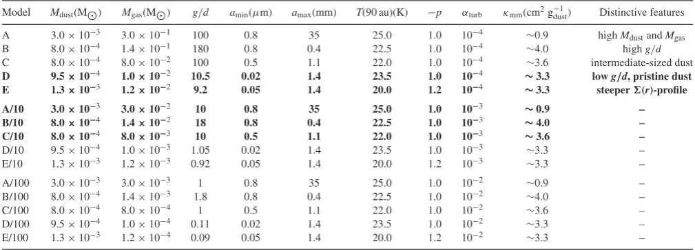
Table 4. Parameters of our 15 models that fit the observed SED:Mdust,Mgas,g/d,amin,amaxandTmid-planeat the location of the CO snowline radiusRsl= 90 au. We also give the power-law exponentpof the surface density profile ∝r−p. We list as well the turbulent mixing strengthαturband the mm opacityκmm of the dust grains that MCMAXis using. The respective distinctive characteristics of the models are given in the last column. Models (A–E)/10 and (A–E)/100 have the same dust properties as models A–E, but theirg/d(and thus theirMgas) are divided by factors of 10 (100) and theirαturbmultiplied by 10 (100) in comparison with models A–E. The models given in boldface are the models that also match the observed C18_{O line profiles as we will discuss in the next} section.

Model Mdust(M) Mgas(M) g/d amin(μm) amax(mm) T(90 au)(K) −p αturb κmm(cm2g−dust1) Distinctive features

A 3.0×10−3 _3.0×10−1 _{100 0.8 35 25.0 1.0 10}−4 _{∼0.9 highMdustandMgas}

B 8.0×10−4 _1.4×10−1 _{180 0.8 0.4 22.5 1.0 10}−4 _{∼4.0 highg/d}

C 8.0×10−4 8.0×10−2 100 0.5 1.1 22.0 1.0 10−4 ∼3.6 intermediate-sized dust

D 9.5×10−4 1.0×10−2 10.5 0.02 1.4 23.5 1.0 10−4 ∼3.3 lowg/d, pristine dust

E 1.3×10−3 1.2×10−2 9.2 0.05 1.4 20.0 1.2 10−4 ∼3.3 steeper(r)-profile

A/10 3.0×10−3 3.0×10−2 10 0.8 35 25.0 1.0 10−3 ∼0.9 –

B/10 8.0×10−4 _1.4×10−2 _{18 0.8 0.4 22.5 1.0 10}−3 _{∼4.0 –}

C/10 8.0×10−4 _8.0×10−3 _{10 0.5 1.1 22.0 1.0 10}−3 _{∼3.6 –}

D/10 9.5×10−4 _1.0×10−3 _{1.05 0.02 1.4 23.5 1.0 10}−3 _{∼3.3 –}

E/10 1.3×10−3 _1.2×10−3 _{0.92 0.05 1.4 20.0 1.2 10}−3 _{∼3.3 –}

A/100 3.0×10−3 _3.0×10−3 _{1 0.8 35 25.0 1.0 10}−2 _{∼0.9 –}

B/100 8.0×10−4 _1.4×10−3 _{1.8 0.8 0.4 22.5 1.0 10}−2 _{∼4.0 –}

C/100 8.0×10−4 _8.0×10−4 _{1 0.5 1.1 22.0 1.0 10}−2 _{∼3.6 –}

D/100 9.5×10−4 _1.0×10−4 _{0.11 0.02 1.4 23.5 1.0 10}−2 _{∼3.3 –}

in every case that the grains follow a power-law size distribution of

n(a)∝a−k_{, whereais the grain size. The value for ISM grains, that}

is often also adopted for discs, isk=3.5 (see e.g. Mathis, Rumpl & Nordsieck1977; Clayton et al.2003), which results in most of the dust mass being in the largest grains, while the opacity is provided by the smallest dust.

We choose to vary these five disc parameters in our modelling as they have the biggest effect on the SED (Meijer et al. 2008, Pani´c et al., submitted). We explore a range ofMdustgoing from

the lowest possible value that can still reproduce the mm flux in the SED as we will describe in Section 4.1 up to∼0.1 per cent of the stellar mass. We initially varyg/dbetween 10and200 to explore an extreme range around the ISM value (while fixingαturb=10−4).

Once we find a combination ofαturbandg/dthat provide a match,

we then explore other combinations of these two parameters, taking into account the above described degeneracy ofαturb×g/d. The

grains sizes we assume range from pristine dust (sub-micron-sized) to mm or even cm-sized grains in some cases.

The stellar properties that we use for all of our models are listed in Table1and are kept fixed. We use a Kurucz model for the star, which sets the stellar emission. Given the values for the outer radius as inferred from CO observations, we use a value of

Rout=540 au for our models. We then investigate how our

parame-ter choices affect the resulting SED and the predicted radius of the CO snowline. Rather than finding the single model that provides the best fit to these observables, we instead identify a range of models that provide an acceptable fit and then, as detailed in the following section, further isolate the models that additionally match the line fluxes in C18_O.

3.1.2 Modelling of the C18_{O line emission}

The models we obtain from the analysis described above are then taken as an input density and temperature structure for the next modelling step. We use the radiation transport and hydrodynam-ics code TORUSto perform molecular line transfer calculations in

this paper (see e.g. Harries2000; Rundle et al.2010; Haworth & Harries2012).TORUSis capable of molecular statistical equilibrium

calculations and the production of synthetic data cubes (e.g. for one specific molecular transition). Full details of the main molec-ular line transfer algorithm are given by Rundle et al. (2010); we summarize key and new features below.

We map the gas density and temperature distributions from the 2D spherical MCMAXcalculations on to the 2D cylindricalTORUS

grid using a bi-linear interpolation inrandθ. We assume that the gas and dust are thermally coupled (allowing us to map the dust temper-ature directly on to the gas). AlthoughTORUSis capable of non-local

thermodynamic equilibrium (LTE) molecular line transport, for ap-plication to these disc models, the densities are sufficiently high and the assumption of LTE produces identical results as non-LTE calculations.3_{Therefore, the level populations can be characterized}

as a Boltzmann distribution, that is as a simple function of temper-ature

ni

ini

= giexp

−Ei

kTgas

zTgas

, (4)

3_{The assumption of LTE is prudent in the mid-plane for mm lines (in which} we are interested as they preferentially probe the disc mid-plane), but might not be sufficient for the infrared (IR) lines.

where gi is the statistical weight and z(Tgas)=

igiexp(−

Ei

kTgas)

the partition function. With the level populations computed, syn-thetic data cubes are calculated using ray tracing (Rundle et al.

2010).TORUSallows for flexible choice of observer viewing angle

and spectral/spatial resolution. We implement a model for freeze-out, whereby the C18_{O abundance drops to a negligible value if}

the temperature is below the freeze-out temperature (which is

Tmid-plane(90 au)) of the respective model. We list these

tempera-tures in Table4. To evaluate the effect of photodissociation of CO by the stellar irradiation, we implement a simple criterion, qualita-tively similar to that of Williams & Best (2014). We assume that for a CO particle column density ofNCO≈1018cm−2in the line

of sight from the star, all CO molecules will be photodissociated. This is only a crude estimate, however, it allows us to check how much of the total gas mass is affected and to gauge the impact on our model. The value we adopt implies a larger role for photodis-sociation than that employed by Williams & Best (2014) (who use

NH2≈1.3×10

21_cm−2_{, corresponding to N}

CO≈1.3×1017cm−2

forfCO≈10−4). We also explore the effect of adopting even larger

column density thresholds ofNCO≈1019cm−2and≈1020cm−2, the

latter of which certainly exaggerates the effect of photodissociation. Turbulence affects the line emission to a much lesser extent than the temperature and density do, and these effects are only marginally discerned in observations of higher signal to noise lines, such as those of12_{CO and at a high spectral resolution. Our assumption of}

turbulent velocityvturbtherefore does not affect our fit to the C18O

data. The maximum turbulent line broadening possible is set by the sound speed in the outer mid-plane

cs= kBTmid(rout)

μmH

, (5)

wherekB is the Boltzmann constant,Tmid the mid-plane

temper-ature,μthe mean molecular weight andmHthe atomic mass of

hydrogen. Following Simon et al. (2015), we employ a value of 0.01–0.1cs, suitable in the outer disc mid-plane, for the turbulent

line broadening inTORUS. Given that the temperature in the outer

mid-plane is approximatelyT≈8 K, we find

vturb=(0.01−0.1)×cs(8 K)=(0.0017−0.017) km s−1, (6)

whereμ=2.37. The recent study by Flaherty et al. (2015) also suggests that turbulence is relatively week in the HD 163296 disc (vturb < 0.03csin the upper layers of the outer disc), supporting

our low value of vturb. Changingvturb by a factor of 10 in our

models does not alter the fit to the observations of C18_{O, as the}

data quality does not allow us to probevturbsufficiently well. Also,

since C18_{O is mainly optically thin, turbulent broadening will cause}

slight smearing of the line profile, but will not affect the line flux. This would be different if we were studying a more optically thick transition like for example CO J= 3–2 (see e.g. Flaherty et al.

2015). The turbulent line broadening is related to the turbulent mixing parameterαturbby

vturb∼ √

αturbcs. (7)

The above means thatαturb=10−4–10−2is implicit in this

calcu-lation. Flaherty et al. (2015) findαturb < 9.6×10−4 from their

modelling of HD 163296. We explore this range of values ofαturb

in Section 4.1, but we hereby stress that for a wide range ofαturb

and corresponding values ofvturbour fit to the line emission remains

Another aspect to take into account is that the fractional abun-dance (by number density) of C18_{O is uncertain. This abundance is}

given by

fC18O=

[CO] [H2]

·[C18O]

[CO] , (8)

where we assume that [C18_O]/[CO]=[18_O]/[16_{O]. Therefore,}

un-certainty in the isotopic ratio of16_{O to}18_{O as well as in the fractional}

abundance of CO have to be taken into account. The abundance of CO is altered due to freeze-out (mid-plane) and photodissociation (surface) (see e.g. Pani´c et al.2008; Miotello et al.2014). The ISM abundance of [CO]/[H2]∼10−4(Aikawa & Nomura2006) is

usu-ally also assumed for discs. However, it is important to note that there is a significant scatter around this value: Lacy et al. (1994) find a maximum value of the fractional abundance of12_{CO of 9.1} ×10−4_{, whereas Frerking et al. (1982) obtain a value of∼8.5×}

10−5_{inρOph and Taurus. Given the isotopic ratio of [}16_O]/[18_O]

and its errors (557±30; Wilson1999), the resulting C18_{O fractional}

abundance we employ is in a range between

1.4×10−7_< [C 18_O]

[H2]

<1.7×10−6_{. (9)}

The maximum effect of this uncertainty on the line emission is achieved in the optically thin case, where the line emission scales linearly with the abundance. We take this fully into account when presenting the results of our calculations of the C18_{O line emission.}

C18_{O J=2–1 is excited by molecular collisions within the disc. The}

shape of its line is thus dependent on the temperature and density structure of the disc and on the C18_{O mass available.}

Using theCASAsoftware package, we further process the data

cubes to obtain synthetic ALMA observations that take into account filtering and instrumental and thermal noise effects. These can then be directly compared with or fitted to the observational C18_{O data}

(e.g. molecular line profiles).

4 R E S U LT S A N D D I S C U S S I O N

4.1 Results of the SED modelling

Initial mass estimate:We have explored in total over 100 models varyingMdust,amin,amaxandg/d(alone, and in combination with αturb) and have found 15 models that fit the observed SED, the

details of the models are given in Table4.

In order to fit our model to the observed SED, we start from an initial estimate of the minimum dust mass, which determines the overall SED shape. If the resulting fluxes in the SED are too high compared to the observations, we decrease the dust mass. If the mm-wavelength fluxes are too high at shorter mm-wavelengths, but not in the mm, we reduce theg/dratio. We then make further improvements on the fit by varying the minimum and maximum grain size, taking into account the effects of the individual disc parameters on the SED. For model series B–E, we have based our initial dust mass estimate on the following considerations: for optically thin emission, the dust mass is given by

Mdust= Sλd2

κλBλ(T), (10)

whereSλis the flux at a certain wavelength,dthe distance of the

source in pc andκλthe opacity at wavelengthλ.Bλis the Planck

function depending on the temperature, given by

Bλ= 2hc

2 λ5 exp hc λkBT

−1

−1

, (11)

wherehis the Planck constant andkBthe Boltzmann constant. For

a distance ofd≈120 pc (van den Ancker et al.1998), temperature

T≈20 K and at a wavelength ofλ≈0.85 mm, we find a flux of Sλ≈2.1 Jy (Guidi et al.2016). We thus estimate a minimum dust

mass ofMdust, min∼8×10−4M. Here, the opacity we assume is

given in Draine (2006), who shows that atλ≈1 mm, dust grains of sizea≈1 mm are most efficient emitters withκλ≈4 cm2_g−1

dust,

as they contain most of the mass (they are, however, not the most efficient emitters per unit mass). Table4shows that this grain size is comparable to the maximum grain sizeamaxof model series C–

E. These models therefore represent the case when the bulk of the mass is in∼1 mm-sized grains andMdustis low. For a grain size

of 0.4 mm as in model series B,κλfrom Draine (2006) is a little lower, leading to a slightly higher minimum dust mass than in model series D to reproduce the same SED. Note, however, that we used the above calculation only to get an initial value forMdust, employing

standardized values for the opacity. The mm opacitiesκmmwe are

using with MCMAXare given in Table4, they depend on the dust

grain size, thus they vary from model to model and differ slightly from the values given in Draine (2006), which are for a material of specific chemical composition and properties assumed to be similar to ISM dust. However, the mm opacities only influence the exact location of the mm point in the SED.

Our models:The SEDs of all our models are given in Fig.2. As discussed above, all models of a given model series have the same SED due to the degeneracy ofαturbandg/d. We include a

zoom-in of the far-zoom-infrared (FIR) and mm region of the SED as this is the wavelength regime that is most crucial for our analysis. All our models match the observed SED in this wavelength range very well, therefore the different models are hardly distinguishable there. We do not try to fit the observed SED at wavelengthsλ2 mm because emission in this regime can be dominated by free–free-emission (Wright et al.2015; Guidi et al.2016), which is not included in our calculations. Note that the only models which can reproduce

the λ >2 mm observations by thermal emission – and no free–

free emission at all – are the models of series A, D and E, where series A needs large grains (35 mm) and all three of them a high dust mass. Furthermore, the models do not match the near-infrared (NIR) excess atλ <10µm very well, but this is sensitive to the exact dust grain composition and geometry of the very inner disc (inner few au; Meijer et al.2008). Including a puffed-up inner disc rim, which could potentially cast a shadow on to the disc surface, might be expected to provide a better fit to the NIR SED. However Acke et al. (2009) find that this would only influence the NIR regime of the SED (not the FIR or mm). Therefore, a puffed-up inner rim would not improve the fit over a substantial wavelength range. The NIR fit does not alter our results for the dust mass, which is calculated using the longer wavelength component of the SED. Furthermore, adjusting the scaleheight in the inner disc would violate the self-consistency of our models. For simplicity, we therefore do not include a model for a puffed up inner rim at this stage.

Description of model series (A, B, C, D, E):We will first discuss the general characteristics of each of these models. We find that model A has a relatively highMdustandMgas(of the order of 10 per cent of the

Figure 2. SEDs of our best-fitting models (parameters can be found in Table4). Due to the degeneracy ofαturbandg/d, the SEDs within each model series are exactly the same (see the text). The observations are plotted as black circles including the respective error bars. The observational data are taken from Berrilli et al. (1992), Mannings & Sargent (1997), Bouwman et al. (2000), Isella et al. (2007), Qi et al. (2011), Tilling et al. (2012), Mendigut´ıa et al. (2012), de Gregorio-Monsalvo et al. (2013) and theSpitzerc2d legacy survey.

ratios, theirMgasvalues differ by about a factor of 2. In order for

them to give the same SEDs, model B with the higherg/dhas to have different grain sizes from model C: its minimum grain size is a little larger than for model C, while its maximum grain size is about a factor of 3 smaller. The distinctive feature of model B is its high

g/dratio which we compensate for by making its minimum grain size bigger than in model C. Therefore – as described for model A – the fluxes in the SED are reduced. Models D and E have a much lower gas mass than the other models we found, but they all have the same SED. This is caused by these two models being the only ones with very small grains. These are coupled to the gas, dragged to higher layers and thus intercept more stellar flux. In general, models A–C have relatively large grain sizes (which probably corresponds to a more evolved state), otherwise the SEDs would produce too high values in the FIR. Model E is similar to model D, but employs a different radial dependence of the surface density: for models series A–D, we assumed ∝r−1_{, for model series E, we take a}

slightly steeper profile ofr−1.2_{, although still well within the range of}

observationally measured values for protoplanetary discs (Andrews et al.2010). Model series E yields a lower mid-plane temperature at the location of the CO snowline radius than the other models, as we will discuss shortly.

We have calculated the optical depth of the continuum emission for our models (using the surface density and mm opacity), which yields that the mm continuum emission for all our models is op-tically thin, except for model series E, where it becomes opop-tically thick within the inner∼10 au. This enables us to obtain a reliable estimate of the dust mass in the disc. We would like to highlight that some of our models reach the maximum mm opacity (as obtained by Draine2006) and are indicative of the minimumMdust∼8×

10−4_M

as derived earlier in this section. Much lowerκmmare of

course possible if a big fraction of the mass is hidden in pebbles and larger bodies, which do not contribute to the mm flux. In such cases,Mdustin our models is just indicative of the mass of the mm

dust and thus a much higher total mass of solids can be achieved. However, such models would not differ in the SED.

Variations of model series (A–E/10, A–E/100):Models A–E have a turbulent mixing strength ofαturb=10−4, but as described above,

we run additional calculations for these models, exploring larger values ofαturb(10−3and 10−2) while decreasing the gas masses in

these models by factors of 10 and 100. We leave all the remaining parameters of models A–E unchanged, as listed in Table4. Indeed, we find that we can match the observational constraints given by the SED and mid-plane temperature requirements by all our models A– E, by changing theMgasand adjusting theαturbaccordingly, to keep

Mgas ×αturb (and therefore the dust diffusion solution, resulting

temperature structures and the SEDs within each model series) constant. In general, all models A–E/10 and A–E/100 yield low to very lowg/dratios by construction. In order to compensate for the lower gas masses, higher levels of turbulent mixing are needed to transport the dust grains to higher altitudes in the disc where they can absorb the stellar light and give the same SED. Given that the dust grain properties within a certain series are exactly the same, our above description of the distinctive features of models A–E holds true for (A–E)/10 and (A–E)/100, respectively.

Figure 3. SED of the whole discR<540 au (red solid line), from within

R < Rdust,850µm=240 au (black dashed line) and fromR<Rsl=90 au (black dash–dotted line).

Meijer et al. (2008), Woitke et al. (2016) and Pani´c et al. (submitted). It is therefore important to note that SED modelling alone does not provide unambiguous physical models of the disc structure, but is highly degenerate.

4.2 Disc regions determining the SED

Fitting observed SEDs in general is most suited for the inner disc regions, since dust grains in the outer disc regions do not intercept sufficient stellar light to contribute substantially to the SED. We have checked that the SEDs as obtained from the whole discs (R=540 au) of our 15 models (as shown in Fig.2), are only marginally changed when taking the emission from within 240 au. This is plotted in Fig.3for model series D, we find the same behaviour for the other models. Thus, the fact that our model discs are described by a single power-law surface density distribution out to 540 au (whereas the observed dust distribution extends only to∼240 au) will not have a significant effect on our SED fits. We will later focus on the gas budget of the disc within the CO snowline (Rsl=90 au) and note

that, in our models, this region contributes around 40–50 per cent of the flux at sub-mm wavelengths. We also overplot the SED for the emission from within the snowline radius in Fig.3.

4.3 Models matching the CO snowline location

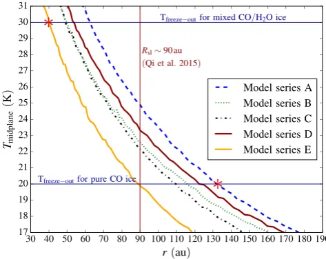
As an additional constraint we have to make sure that our MCMAX

models are consistent with the observed CO snowline location. Therefore, we analyse the mid-plane temperature profileTmid-plane(r)

for all our models that match the observed SED, which we plot in Fig.4. As mentioned above, models of the same series have the same temperature structure. We find that all of them have mid-plane tem-peratures between∼20and25 K at the observed snowline radius of

Rsl≈90 au (Qi et al.2015). These are well within the range of

values generally assumed and observed for the freeze-out tempera-ture of CO: The freeze-out temperatempera-ture can vary between∼20 and

∼30 K depending on whether CO is binding to pure CO ice or a mixture with water ice (Collings et al.2004), which is, in turn, also dependent on the chemical history of the ice (Garrod & Pauly2011). In general, the CO freeze-out temperature is not known unambigu-ously and might vary from system to system (Hersant et al.2009; Qi

Figure 4. Mid-plane temperature as a function of radius for our 15 disc models that match the observed SED. Models from the same series have exactly the same mid-plane temperature structure (see Section 3.1.1). In dark red (vertical), we plot the observed snowline radius≈90 au (Qi et al.

2015). The upper and lower limits of the freeze-out temperature (∼20–30 K) as found by e.g. Collings et al. (2004) are plotted as horizontal lines. The red asterisks indicate where the snowline location could be between∼40 and 135 au due to a plausible range of freeze-out temperatures of 20–30 K if the snowline location was not known unambiguously from observations.

et al.2015): Qi et al. (2013a) found a freeze-out temperature of CO of 17 K from their modelling of TW Hya, whereas Jørgensen et al. (2015) obtain temperatures of about 30 K in their study of embed-ded protostars. Qi et al. (2011) assume a freeze-out temperature for CO ofT≈19 K (pure CO ice) for HD 163296. However, in Qi et al. (2015), they perform a new analysis with higher resolution obser-vational data and use a temperature in the mid-plane atRslofT≈

25 K (mixed CO/H2O ice). Thus, all our models have temperatures

in the disc mid-plane at the location of the snowline radius that are well within the plausible range. Our exploration of self-consistent models confirms that all the freeze-out temperatures assumed in these previous literature references fall within the plausible range of temperatures for HD 163296. If the freeze-out temperature of CO was known unambiguously, this would, in combination with an observationally determined CO snowline location, be a powerful model discriminant and we might be able to exclude models based on this constraint. Since, however, it is unclear what exactly the relevant freeze-out temperature is, we find that all the models can match the observed snowline location of 90 au. This weak model discrimination also means that it is impossible to predict the CO snowline radius from SED model fitting alone or even from fitting the molecular line emission together with the SED (Qi et al.2011): given the uncertainty in the sublimation temperature of CO, our viable SED fits imply predicted radii in the range∼40–135 au as denoted by the red asterisks in Fig.4. In general, we find that the location of the CO snowline radius does not further discriminate between models in comparison to the criterion given by the SED; however, it sets the radial location inwards of which no freeze-out is taking place in our models, and which is therefore important for the interpretation of the C18_{O emission. It is important to note that an}

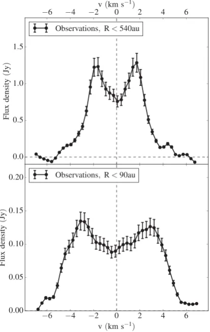
Figure 5. C18_{O J=2–1 line profile (ALMA observations) using the} emis-sion from the whole disc (upper panel) and from within the 90 au snowline radius. The error bars represent a 10 per cent flux calibration uncertainty (Guidi et al.2016). We centred the spectra on 0 km s−1_{. The systemic} velocity isvsys=5.8 km s−1.

We conclude that all our 15 models match the SED and CO snow-line location within the uncertainties in the freeze-out temperature. The SED modelling is especially powerful for the inner∼240 au and describes the disc structure inside the CO snowline location well.

4.4 C18_{O J=2–1 emission}

4.4.1 C18_{O line profiles}

As discussed in Section 3.1.2, we use the density and temperature structures of our MCMAXmodels to calculate the C18O line emission

withTORUS. The aim of our work is to interpret the observed C18O

J=2–1 line profile, especially from the inner disc regions, in the context of a physically consistent model that matches other relevant observations (Rsl, SED). We show the C18O J=2–1 line profile as

observed by ALMA in Fig.5, both taking the emission from the whole disc and from within the 90 au snowline radius. These are very different, especially in the peaks of the spectrum, as these are dominated by the emission from the outer disc regions. Our goal is to model the disc regions withR<90 au (the snowline location), as these are independent of the details of freeze-out in the outer disc.

Uncertainty in abundance of C18_{O: As mentioned previously, the}

fractional abundance of C18_{O has a large uncertainty and is observed}

(in star-forming clouds) to be in a range between 1.4×10−7_and1.7 ×10−6_{(see Section 3.1.2), thus spanning an order of magnitude.}

From matching the observed C18_{O J=2–1 line profile with our}

models, we can unambiguously calculate the mass of C18_{O in the}

disc. However, when converting this mass to a mass of H2, we will

have to take into account this range of C18_{O abundance.}

Matching the observed C18_{O line profile, we find that – taking}

into account the range of plausible abundances – only five of our models can fulfil this criterion, namely (A–C)/10, D and E. We will thus focus on these models in the further discussion.

Another aspect to take into account is that the abundance of C18_O

in comparison to H2can be altered due to freeze-out in the disc

mid-plane, as already discussed in the previous section. We have implemented this effect inTORUSby setting the abundance of C18O

to a negligible value when the disc temperature drops below the freeze-out temperature. For the individual models, we use the mid-plane temperature of the respective model at the observed snowline radius as given in Fig.4. The fraction of the C18_{O mass removed by}

freeze-out in the respective models is given in Table5. We find that this effect is stronger for models (A–C)/10 than for models D and E, because the former have slightly higher gas masses and bigger grains, thus a higher fraction of the mass will be concentrated in the cooler disc mid-plane regions and thus subject to freeze-out. However, the exact impact of freeze-out on the line profile will depend on the details of the vertical temperature profile and thus on the location of the CO ice surface.

The second most relevant source of CO-removal from the gas-phase is photodissociation (Visser, van Dishoeck & Black2009; Miotello, Bruderer & van Dishoeck2014). As described in Sec-tion 3.1.2, we have taken this into account in our modelling. We do this by setting the C18_{O abundance to a negligible value for a}

threshold column density of gas calculated from the star in dif-ferent azimuthal directions covering the entire disc height. These threshold column densities vary fromNCO=1018cm−2, 1019cm−2

and 1020_cm−2_{(corresponding to 10}22_H

2cm−2, 1023H2cm−2and

1024 _H

2cm−2, respectively, assumingfCO ∼10−4). We find that

overall only a small fraction of C18_{O is photodissociated within the}

90 au snowline location in our models. For the first threshold, the fraction of the CO gas mass photodissociated is∼0.1 per cent in all our models, forNCO=1019 cm−2, it is∼1 per cent and even

for the extreme case, only∼3 per cent is photodissociated within the snowline radius. We calculate the C18_{O line emission forR<}

90 au after removing CO from the photodissociated layer, in the three explored cases (NCO=1018cm−2, 1019cm−2and 1020cm−2).

This is presented for the example of model D in Fig.6. Given that, in our analysis, we mostly focus on the regions within the 90 au snowline radius that are not subject to freeze-out and not strongly affected by photodissociation, our models are not dependent on the exact details of these processes.

The inner disc regions (R <90 au): For 5 out of our 15 initial models, we can match the observed C18_{O J=2–1 line profile within}

the range of plausible C18_{O abundances between 1.4 ×10}−7_and

1.7×10−6_{(equation 9). We show the C}18_{O spectra arising from}

the regions inside the 90 au snowline radius in these models in the left-hand panels of Fig.7. We will call these five models (A– C)/10, D and E ‘fiducial’ models in the further discussion. We obtain these from the synthetic and ALMA data cubes using the

CASAsoftware in the following way: we calculate the emission from

en elliptical region, centred on the centre of the disc using a PA= 132◦and a ratio of minor to major axis b

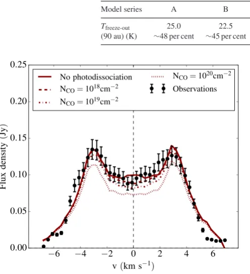
Table 5. Freeze-out temperatures (mid-plane temperatures at 90 au) and fractions of the CO mass removed in the various model series due to freeze-out.

Model series A B C D E

Tfreeze-out 25.0 22.5 22.0 23.5 20.0

(90 au) (K) ∼48 per cent ∼45 per cent ∼40 per cent ∼27 per cent ∼23 per cent

Figure 6. C18_{O flux density for model D (from regions withR<Rsl=} 90 au) employing different column density thresholds for photodissocia-tion: no photodissociation (solid),NCO=1018_cm−2 _{(dashed), 10}19_cm−2 (dash–dotted) and 1020_cm−2_{(dotted). Even in the most extreme case, only} ∼3 per cent of the CO mass is affected. For reference, we also plot the observed line profile for this disc region, given by the black points with error bars (10 per cent flux calibration uncertainty). We find a very similar behaviour for the other models and thus do not show the respective plot here.

These values of PA and inclination are the ones we obtained in the analysis of the observations (see Section 2). All of them match the observations well within the error bars (given by the∼10 per cent flux calibration uncertainty of the ALMA observations; Guidi et al.

2016). The fractional abundances of C18_{O of these models can be}

found in Table6. Given these abundances and the gas masses in the respective models, we can calculate the mass of C18_{O within the}

snowline radius, as the C18_{O J=2–1 transition is mainly optically}

thin throughout the whole disc. We have calculated the optical depth of the C18_{O J=2–1 transition and found that it is indeed}

optically thin throughout the whole line profile and at all radii for all our models that match the observations. Although the models are optically thin, this would not have been a necessary precondition for our modelling process as the radiative transfer calculation self-consistently accounts of optical depth effects. However, the low optical depths emphasizes how essential C18_{O is as a tracer for the}

disc mid-plane. That implies that we can unambiguously calculate theMC18_Owithin 90 au which should be approximately the same

for all our models. The values we obtain are listed in Table6and are in a range of

MC18O(R <90 au)≈2−3×10−8M. (12)

The values that Qi et al. (2011) obtain for these inner disc regions are comparable to ours. In the right-hand panels of Fig.7, we plot the emission from a bigger disc region, namely from within the

outer dust radiusRdust≈240 au. Our models still closely match the

wings of the spectrum and thus the emission from the inner disc regions. However, one can see that our models slightly overpredict the emission from the outer disc regions (i.e. in the peaks of the spectrum) there. The height of the peaks depends crucially on the exact vertical temperature structure of the models as freeze-out will reduce the C18_{O emission, especially in the outer disc regions.}

However, we do not attempt to match these disc regions, but focus on the innermost 90 au.

Models with minimum and maximum g/d: So far, we have only explored the five models from our initial Table4that also match the C18_{O line profile. However, it is interesting to look into the extreme}

cases, i.e. models with minimum and maximum plausible C18_O

abundance (and thus maximum and minimumg/dandMgas), while

still matching the observed C18_{O and thus the C}18_{O masses within}

90 au we just calculated. We give the properties of the extreme models in Table7. It is important to note that models Dmaxand Emax

can be excluded as theirαturbis lower than the minimum of 10−4we

assume. Models D and E both have this minimum value; therefore for model series D and E, the highest possible values ofg/dand thereforeMgaswithin 90 au are the ones given in Table6. The highest

possible values ofg/dfor models that match the observed C18_{O line}

profiles are 82 and 71 (for models Bmaxand Cmax, respectively); the

lowest value is 2 (model Amin). We take these three cases into

account for the further discussion as they are the extreme ends of theg/drange we obtain.

Modelling the entire disc: Finally, for completeness, we compare the synthetic line profile for the whole disc with observations in Fig.8. We see that our models overpredict the emission from the outer disc regions, i.e. the emission in the peaks of the spectrum. However, as we mentioned earlier, the SED does not provide in-formation about the structure of the outermost disc regions. Also, we know that there are radial differences in the structure of the outer disc and the inner 240 au and we therefore limit our attention to the disc inner regions in this paper. It might be interesting to combine our modelling approach for the inner disc regions with high-resolution imaging of multiple isotopologues in the outer disc regions (see e.g. Qi et al.2011; de Gregorio-Monsalvo et al.2013).

4.4.2 Physical properties of our models

Gas mass within the snowline radius: The match to the observed C18_{O spectrum within the CO snowline which we find for our five}

models unambiguously constrains the mass of C18_{O in this disc}

region. In equation (12), we gave this mass within the snowline radius. We thus calculate the mass of H2in this disc region from MC18_O(90 au) by taking into account the abundance of C18O given

in Table6and the mass ratio of these moleculesmC18O/mH2≈14.

We find that the mass of H2within the snowline radius is in a range