Comparison of linear and nonlinear implementation of the compartmental tissue uptake model for dynamic contrast-enhanced MRI.

Comparison of Linear and Nonlinear Implementation of

the Compartmental Tissue Uptake Model for Dynamic

Contrast-Enhanced MRI

Jesper F. Kallehauge,

* Steven Sourbron,

Benjamin Irving,

Kari Tanderup,

Julia A. Schnabel,

and Michael A. Chappell

Purpose: Fitting tracer kinetic models using linear methods is much faster than using their nonlinear counterparts, although this comes often at the expense of reduced accuracy and precision. The aim of this study was to derive and compare the performance of the linear compartmental tissue uptake (CTU) model with its non-linear version with respect to their percentage error and precision. Theory and Methods:The linear and nonlinear CTU models were initially compared using simulations with varying noise and temporal sampling. Subsequently, the clinical applicability of the linear model was demonstrated on 14 patients with locally advanced cervical cancer examined with dynamic contrast-enhanced magnetic resonance imaging.

Results:Simulations revealed equal percentage error and pre-cision when noise was within clinical achievable ranges (con-trast-to-noise ratio>10). The linear method was significantly faster than the nonlinear method, with a minimum speedup of around 230 across all tested sampling rates. Clinical analysis revealed that parameters estimated using the linear and non-linear CTU model were highly correlated (r0.95).

Conclusion:The linear CTU model is computationally more efficient and more stable against temporal downsampling, whereas the non-linear method is more robust to variations in noise. The two methods may be used interchangeably within clinical achievable ranges of temporal sampling and noise. Magn Reson Med 000:000–000, 2016.VC_{2016 The Authors Magnetic Resonance in Medicine}

pub-lished by Wiley Periodicals, Inc. on behalf of International Soci-ety for Magnetic Resonance in Medicine. This is an open access article under the terms of the Creative Commons Attribution License, which permits use, distribution and reproduction in any medium, provided the original work is properly cited.

Key words: DCE-MRI; tracer kinetic modeling; pharmacoki-netics; cervical cancer; linear least-squares method; nonlinear least-squares

INTRODUCTION

Dynamic contrast-enhanced MRI (DCE-MRI) is a power-ful tool to evaluate tissue perfusion, permeability, and vasculature. High temporal resolution scans are per-formed while a gadolinium-based contrast agent is intro-duced into the patient’s blood stream, and its subsequent uptake is recorded. Numerous methods of analyzing the temporal tissue enhancement profile have been proposed, including phenomenological, semiquantitative, and quan-titative tracer kinetic models (1,2). The most commonly used tracer kinetic models are the Tofts and extended Tofts models, which have proven useful in a variety of clinical applications (3,4). The limitations of the extended Tofts model have been revealed recently, as experimental evidence has shown that this model often fits poorly to data measured at high temporal resolution (5).

This has recently raised an increased interest in the use of more general models, such as the two-compartment exchange model (2CXM) (6). The 2CXM allows for the description of two distinct compartments (veand vp) and separation of flow (Fp) and the permeability surface area product (PS). For reliable estimation of all four parameters, a good contrast-to-noise ratio (CNR), high temporal resolu-tion, and sufficiently long scan duration is required (7). The compartmental tissue uptake (CTU) model is a special case of the 2CXM which applies particularly for data with shorter scan durations (8,9). This model has only three parameters (Fp, PS, vp) and can be applied whenever the acquisition time is shorter than the contrast agent’s extravascular transit times (typically in the range of 2–3 min, but significantly extended in some pathologies). The CTU model is a direct generalization of the well-known Patlak model (10), which applies to data with poorer tem-poral resolution. An important application of the CTU model may be in tissues that include necrosis or cell mem-brane rupture where the contrast agent is captured for a long time. In those cases it is practically impossible to measure long enough to capture the washout phase.

Regardless of the choice of model for data analysis, the parameter estimation is often performed using a nonlinear fitting algorithm. Nonlinear methods require an initial guess of the parameters to be estimated and may converge only to a local minimum. Conversely, linear methods determine the kinetic parameters by solving a set of linear equations, as exemplified by Murase (11) and Flouri et al. (12) for DCE-MRI, and there is also extensive experience in nuclear medicine (13). This is often much faster than the nonlinear approaches, as the optimum can be identified analytically by a single matrix inversion in a closed-form

1

Institute of Biomedical Engineering, Department of Engineering Science University of Oxford, Oxford, United Kingdom.

2

Division of Biomedical Imaging, University of Leeds, Leeds, United Kingdom.

3

Department of Oncology, Aarhus University Hospital, Aarhus, Denmark.

4

Division of Imaging Science and Biomedical Engineering, King’s College London, London, United Kingdom.

Grant sponsors: CRUK/EPSRC Cancer Imaging Centre at Oxford (C5255/ A16466), Danish Cancer Society (R123-A7721), Danish Society of Clinical Oncology.

*Correspondence to: Jesper Folsted Kallehauge PhD, Institute of Biomedi-cal Engineering, Department of Engineering Science, University of Oxford, Old Road Campus Research Building (off Roosevelt Drive), Oxford, OX3 7DQ. E-mail:[email protected]

Received 22 February 2016; revised 10 May 2016; accepted 8 June 2016 DOI 10.1002/mrmt.26324

Published online 00 Month 2016 in Wiley Online Library (wileyonlinelibrary. com).

VC _{2016 The Authors Magnetic Resonance in Medicine published by Wiley}

Periodicals, Inc. on behalf of International Society for Magnetic Resonance in Medicine

Magnetic Resonance in Medicine 00:00–00 (2016)

solution, rather than iteratively via gradient-descent type methods. The drawback often encountered with linear approaches is the higher sensitivity to noise and possible bias due to differences in data weighting (14). The nature and severity of the problem is model dependent, but these issues have not yet been investigated in the specific con-text of the CTU model.

The aim of this study was to formulate the CTU model in a linear form and compare the precision and percentage error of the parameter estimates of both linear and nonlinear solutions. The evaluation was performed using simulations with various noise levels and temporal downsampling. The applicability of the linear approach was demonstrated on 14 clinical cases of locally advanced cervical cancer.

THEORY

The CTU model is a special case of the 2CXM, which is valid whenever the indicator concentration in the plasma volume (vp) is much larger than that in the extravascular distribution volume (ve) (i.e., cp >> ce). It is governed by the following set of coupled linear differ-ential equations:

vp

dcpðtÞ

dt ¼ PScpðtÞ þFpðcaðtÞ cpðtÞÞ [1]

ve

dceðtÞ

dt ¼PScpðtÞ; [2]

where PS is the permeability surface area, Fp is the

plasma flow andcais the concentration in the supplying

artery. The total concentration measured (C) is the com-bination of concentration in the plasma and the extracel-lular and extravascular volume:

CðtÞ ¼vpcpðtÞ þveceðtÞ: [3]

The analytical solution to the CTU kinetic model has been shown previously to have the following form (9):

CðtÞ ¼caðtÞ ðFpet=TpþKtransð1et=TpÞÞ; [4]

where is the convolution operator, Tp is the plasma

transit time also given as the ratio Tp¼_Fpvp_þPS, E is the extraction fraction also given as E¼ PS

PSþFp, and K

trans _is

the volume transfer constant and can be written as Ktrans_¼EF

p.

Linear Solution

By combining the coupled set of linear differential Equa-tions [1] and [2] with Equation [3], we may derive the linear solution to the CTU model.

Substitute in Equations [1] and [2] into the derivate of Equation [3]:

dCðtÞ

dt ¼ PScpðtÞ þFp

caðtÞ cpðtÞ

þPScpðtÞ

¼Fp

caðtÞ cpðtÞ

:

[5]

Differentiating once more and substituting in dcpðtÞ dt iso-lated from Equation [1] yields:

d2_CðtÞ dt2 ¼Fp

dcaðtÞ

dt

Fp

vp

PScpðtÞ þFpðcaðtÞ cpðtÞÞ

:

[6]

Further isolating cpðtÞ in Equation [5] and inserting into Equation [6], we have:

d2_CðtÞ dt2 ¼Fp

dcaðtÞ

dt þ FpPS

vp

caðtÞ

FpþPS

vp

dCðtÞ

dt [7]

Integrating Equation [7] twice over time gives an equa-tion of the form:

C¼ aCþbcaþgca; [8]

whereC andca denote the integral ofC and ca, respec-tively, over time andca is the double integral of ca over time. From the parameters (a;b;g) the following relations for (vp; Fp; PS;Tp; E) may be found:

vp¼ b2

abg; Fp¼b; PS¼ gb

abg ; Tp¼ 1 a; E¼

g ab :

[9]

Equation [8] is a linear equation and may be expressed in matrix form as

c¼Ab: [10]

The least-squares solution can be found by solving the following problem using standard techniques:

min

b jjAbcjj 2

[11]

In the context of the CTU model,A,b, andc would be given as

A¼

Cðt0Þ caðt0Þ caðt0Þ

Cðt1Þ caðt1Þ caðt1Þ

⯗ ⯗ ⯗

CðtN1Þ caðtN1Þ caðtN1Þ 2 6 6 6 6 6 4 3 7 7 7 7 7 5 [12] b¼

PSþFp

vp

Fp

FpPS

vp 2 6 6 6 6 6 6 4 3 7 7 7 7 7 7 5

i:e;

a b g 2 6 6 4 3 7 7 5 and c¼

Cðt0Þ

Cðt1Þ

⯗

CðtN1Þ 2 6 6 6 6 6 6 6 4 3 7 7 7 7 7 7 7 5 ;

whereNis the number of time points. Becausecis pro-portional to the extraction fraction E, which is defined for 0 E 1 a solution withc 0 is consistent with a

one-compartmental state where either; no contrast agent extravasates, the contrast agent exchanges rapidly or the tissue is weakly vascularised (15).

METHODS

Simulation Data

Synthetic concentration curves were generated (Fig. 1a– c) using Equation [4] with a noiseless input function from Parker et al. (16) with a 20-s baseline and 4-min postinjection duration. The temporal resolution was ini-tially set at 10 ms before downsampling, and Gaussian noise was added to the tissue concentration curve C and ca to imitate more realistic clinical scenarios. The data were downsampled to a range of temporal resolutions in the interval Dt ¼ (0.05–10 s) in 0.05-s increments, and the onset time was varied randomly within the chosen resolution (Dt) for all simulations. The CNR was defined as the maximum difference in indicator concentration in the tissue divided by the standard deviation of the base-line noise and was simulated over a range of values (CNR values ranging from 2 to 40). The convolution operation was performed explicitly assuming an expo-nential decay for one of the functions as previously shown by Flouri et al. (12). Three different tissue enhancement curves were considered, corresponding to

previously reported values extracted using the CTU model (summarised in Table 1).

The simulations were performed using MATLAB (MathWorks, Natick, Massachusetts, USA) on an Intel Xeon 2-core (2.4 GHz) with 20 GB RAM, and computa-tion time was measured using the funccomputa-tions tic() and toc(). For the nonlinear parameter estimation, the lsqnon-lin() function in MATLAB along with the Trust Region Reflective algorithm with bounds fixed for the Fp, PS,

and vp parameters to be real positive values (17) was

used (and is referred to hereafter as NLLS). The initial starting guess supplied for NLLS was chosen to be the “true” values used to generate the synthetic data in order to avoid convergence to an unwanted local minimum. This means giving the NLLS a best case scenario with respect to parameter estimation and time to convergence, which may not reflect clinical reality. In other words, we compare the best possible performance of the NLLS with

Table 1

Parameters Used for Simulation

Fp

(min1) vp

PS

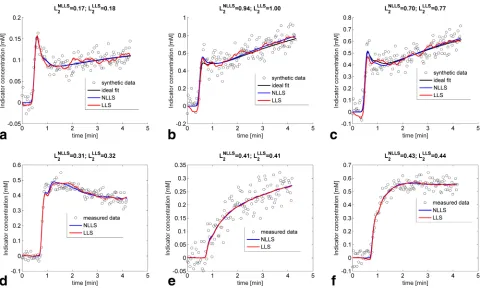
(min1) Reference Brain (tumor) 0.23 0.05 0.02 Sourbron et al. (9) Cervix (tumor) 0.57 0.28 0.2 Kallehauge et al. (23) Cervix (tumor) 0.65 0.22 0.14 Donaldson et al. (5) FIG. 1. Example of the differences in fits between LLS and NLLS. (a–c) CNR was fixed at 10 and the temporal sampling at 2 s. The cor-responding parameters were extracted from (a) Sourbron et al. (9), (b) Kallehauge et al. (23), and (c) Donaldson et al. (5) as summarised in Table 1. The L2-norm showed slightly superior fits of NLLS over LLS for the simulated curves. (d–e) Clinical data curves reflecting dif-ferent types of enhancement. The corresponding parameter estimates for NLLS and LLS were as follows: (d)Fp (NLLS)¼0.76 min1,

Fp(LLS)¼0.72 min1,vp(NLLS)¼0.26 min1,vp(LLS)¼0.26 min1,PS(NLLS)¼0.03 min1,PS(LLS)¼0.03 min1. (e)Fp(NLLS)¼

0.11 min1,Fp(LLS)¼0.11 min1,vp(NLLS)¼0.17 min1,vp(LLS)¼0.18 min1,PS(NLLS)¼0.06 min1,PS(LLS)¼0.06 min1. (f)

Fp(NLLS)¼0.48 min1,Fp(LLS)¼0.50 min1,vp(NLLS)¼0.36 min1,vp (LLS)¼0.35 min1,PS(NLLS)¼0.05 min1,PS (LLS)¼

that of the linear least squares (LLS). The LLS solution was implemented by first calculating all the inputs forA (Equation [12]) using trapezoidal integration. The solu-tion vectorbwas subsequently determined using analyti-cal matrix inversion of the 3-by-3 matrixATA, whereAT is the transpose ofA. The goodness-of-fit was compared using the Euclidean distance (L2-norm) between the data and the fit as estimated from Equations [4] and [8] for NLLS and LLS, respectively. All simulation code can be found online at https://github.com/Jkallehauge/Linear-CTU.

Statistical Analysis

A Monte Carlo simulation of 1000 runs with different random noise was performed for each condition of tem-poral downsampling and noise level. For each of the 1000 runs, the estimated values for Fp, PS, and vp were

calculated using the linear and nonlinear approach and compared. The systematic and stochastic variation in parameter estimations were evaluated using precision and percentage error, which is here defined as

Precisionð%Þ ¼s

m100

Errorð%Þ ¼xm

m 100;

wherexis the parameter value for each of the 1000 sim-ulations, r is the standard deviation of x, and l is the “true” value from which the synthetic data have been generated.

Clinical Data

The clinical applicability was investigated in a prospec-tive study approved by the local medical ethics research board, with written informed consent from all patients. A total of 14 patients with locally advanced cervical cancer were scanned within one week of the start of chemoradio-therapy using MRI on a 3T Philips Achieva-X scanner. DCE-MRI was performed using a three-dimensional axial nonselective saturation recovery spoiled gradient echo technique with the following parameters: number of slices ¼ 20; slice thickness¼ 5 mm; repetition time¼ 2.9 ms; echo time¼ 1.4 ms; Tsat ¼ 25 ms; flip angle ¼ 10 ;

in-plane resolution¼2.3 2.3 mm; and time resolution¼ 2.1 s. The bolus injected was 0.1 mmol/kg Dotarem at 4 mL/s, followed by a 50-mL saline flush. A total of 120 dynamic scans were obtained, of which an average of 18 time points were scanned before the bolus arrived at the external iliac arteries. A T1 relaxation map was con-structed [following Deoni et al. (18)] before contrast agent injection using a three-dimensional gradient recalled echo sequence with five different flip angle scans (5, 10, 15 , 20, 25 ) with the same orientation and field of view as the dynamic scan, a repetition time of 20 ms, and an echo time of 1.7 ms. The dynamic magnitude images were sub-sequently converted into contrast agent concentrations as described previously (19). The regions of interest were chosen to be the clinical gross tumor volume delineated by an experienced oncologist on a transversal

T2-weighted MRI, following the recommendations of the GEC-ESTRO working group (20). In each patient, an arte-rial input function (AIF) was derived by averaging the measured voxelwise AIFs over a number of included vox-els in the left femoral arteries where the B1 field was con-sistently most homogenous (inspected qualitatively). Specifically for the AIF, the precontrast longitudinal relaxation (T1,0) determination was connected with some uncertainty, and a literature value for T1,0 was chosen instead: T1,0(blood)¼1660 ms (21). For the remaining tis-sue curves, the estimated T1-map was used for the conver-sion from signal to contrast concentration. To correct for differences in large and small vessel hematocrit, the AIF was multiplied by a factor 1.18, based on an assumed hematocrit of 0.38 and an assumed small-to-large vessel ratio of 0.7 (22). The clinical data were analysed using both LLS and NLLS.

RESULTS

Synthetic Data

Figure 1a–c shows three example simulations using a temporal resolution of 2 s, where the total acquisition time was 260 s with a baseline of 20 s, CNR ¼ 10, and kinetic parameters corresponding to those in Table 1. Both the NLLS and LLS fits described the synthetic data similarly with only a small difference in the L2-norm (LNLLS

2 andLLLS2 ).

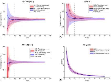
The difference between the true values and derived parameters using both NLLS and LLS under varying noise conditions are summarised in Figure 2. Figure 2a shows the results forFp where the LLS underestimates the true

value ofFpunder noisy conditions (CNR<10), whereas

NLLS tends to overestimate Fp under very noisy

condi-tions (CNR<5). At high CNR values, LLS approximates the true value better than NLLS. The precision of estimat-ing Fp was consistently better for NLLS for CNR > 10.

Both NLLS and LLS overestimated the true value of vp

(Fig. 2b), although NLLS less so than LLS for low CNR (CNR< 15). The two curves converge around CNR 15 after which little difference between the two curves is seen both in terms of percentage error and precision. The influence of noise on PS was also lower for NLLS com-pared with LLS under low noise conditions, and above CNR¼10 their precision and percentage error were com-parable (Fig. 2c). The overall effect of noise on the quality of the fit (Fig. 2d) was measured using the L2-norm and showed comparable performance across all CNR values.

The percentage error and precision for the three differ-ent tissue types (see Table 1) are summarised in Table 2 for a realistic temporal resolution and noise level (Dt¼2 s and CNR¼10, corresponding to the vertical dashed lines in Fig. 2). Both NLLS and LLS underestimated the true val-ues ofFpfor the three tissue types, with only marginally

better precision and percentage error for NLLS over for LLS.vp was generally overestimated across all simulated

tissues, however, to a lesser degree for NLLS. The preci-sion ofvPwas again better for NLLS. The percentage error and precision ofPSestimated using both NLLS and LLS were comparable and with almost no bias.

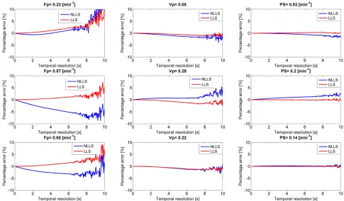
The effect of temporal downsampling as examined on noiseless data is shown in Figure 3. For the higher tested

tissue values of Fp (0.57 min1 and 0.65 min1), LLS

was less influenced by temporal downsampling than NLLS while for the low valueFp (0.23 min1) NLLS was less influenced. Almost no influence of temporal sam-pling was observed for vp and PS for lower temporal sampling. Above a temporal period of 8 s, both LLS and NLLS begin to show oscillations corresponding to the width of the Parker input function (8.4 s) (16). The speed improvement of the LLS approach was, over all temporal resolutions and tested parameter configura-tions, at minimum around 230 times faster than the NLLS (Supporting Fig. S1).

Clinical Data

Figure 1d–f shows three clinical example curves with lit-tle difference in the performance of the LLS and NLLS.

The three curves were chosen to reflect different capil-lary transit times: fast (Fig. 1d), slow (Fig. 1e), and inter-mediate (Fig. 1f). Figure 4 shows a comparison of the kinetic maps derived using both LLS and NLLS for a sin-gle central slice through a patient’s tumor. The maps show very similar patterns, suggesting the two approaches can be used interchangeably (see also Sup-porting Figure S3a–n).

By aggregating the data from all 14 patients, a total of 34,525 tumor voxels were analysed using both LLS and NLLS (see overview in Supporting Fig. S2). A subset of these voxels were excluded if they had a negative distri-bution volume (vd¼RCðtÞdt=RcaðtÞdt) or the model fit was completely contained within the 95% confidence interval of the baseline noise. The remaining 32,190 vox-els had a median CNR of 17.4 (95% confidence interval: 6.9, 35.8). LLS returned unrealistic negative values ofFp, FIG. 2. Influence of noise on the percentage error and precision of each hemodynamic parameter (a–c) and the overall fit (d) when applying both NLLS and LLS. The vertical black lines correspond to the values shown in Table 2 (middle row).

Table 2

Percentage Error and Precision for Different Tissue Types atDt¼2 s and CNR¼10

Fp(min1) vp PS(min1)

NLLS LLS NLLS LLS NLLS LLS

PS, and vp in a considerable proportion of the 32,190

voxels, whereas the NLLS was constrained to be within the set boundary points of the fitting algorithm. Discard-ing the regions where the CTU model is not defined (i.e., where vp < 0 or E was not between zero and 1 as

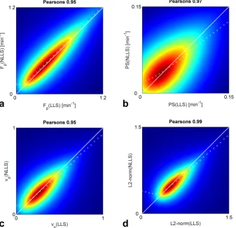
esti-mated by LLS [25,325 voxels left]), we found good agree-ment between NLLS and LLS (Fig. 5). The white dashed line shows the identity line, and the white cross marks () illustrate where the mode or most frequent parame-ters are seen, thus indicating whether LLS over- or underestimates compared with NLLS within in a given range of parameters. Figure 5a generally shows that LLS

and NLLS agreed well over a large range ofFp, and only

at low values does it suggest thatFp is overestimated by

NLLS compared with LLS. Similar findings are seen in Figure 5b,c forPSandvp, although they also suggest that

LLS overestimates the parameter values at high values compared with NLLS. The L2-norm also showed good agreement with a Pearson’s correlation of 0.99. The excluded voxels from the final comparison between the NLLS and LLS were investigated further. Supporting Fig-ure S4 shows example curves of the regions with nega-tive extraction fraction, regions with extraction fraction greater than one, and regions with negative plasma

FIG. 3. Effect of temporal downsampling on both LLS and NLLS for the three different simulated tissue types from Table 1.

FIG. 4. Comparison of hemodynamic maps estimated and goodness-of-fit using both NLLS and LLS. The white center corresponds to data with negative distribution volume or a fit completely contained within the 95% confidence interval of the baseline noise.

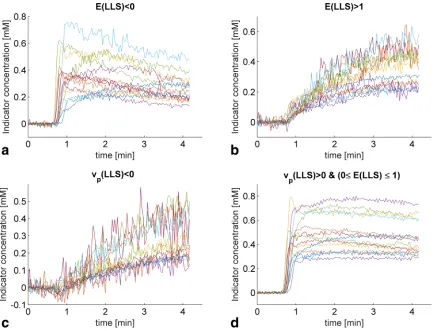
volume fraction. Similarly, Figure 6 shows the patient-wise median curves of the aforementioned regions along with the patient-wise median curves of the data included in the comparison of NLLS and LLS. Generally, the regions with E (LLS) < 0 showed significant washout, whereas the regions with E (LLS) > 1 showed slow enhancement, which may be described adequately by a more simple model (e.g., a one-compartment model). The regions that had a negative plasma volume fraction again showed slow enhancement, with a slight decrease in the initial indicator concentration. A quantitative comparison of the different parameters in the different regions can be found in Table 3. Here, the CNR level was seen to be lower in the regions excluded compared with the included regions. The plasma transit time esti-mated by NLLS [Tp (NLLS)] was furthermore consider-ably longer in the regions whereE(LLS)> 1 orvp(LLS) < 0. WhereasE (LLS)< 0, the Tp (NLLS) was

compara-ble to that of the included voxels, although with a much larger confidence interval. A similar result was observed for Fp (NLLS). Where vp (LLS) was negative, vp (NLLS)

similarly returned unrealistic values with a median that was greater than 1.

DISCUSSION

Principal Findings

In this study, we derived and evaluated the precision and percentage error of a linearised CTU kinetic model.

Specifically, we compared the effects of temporal down-sampling, varying noise, and different tissue hemody-namic parameters on the precision and percentage error of both a nonlinear and linear CTU model. Within the clinical achievable ranges (CNR10) and temporal reso-lution (Dt 2 s) (23), LLS showed comparable perform-ance in terms of percentage error and precision compared with NLLS. Parameters estimated using LLS were generally more stable to temporal downsampling (Fig. 3), whereas NLLS was consistently more stable to variations in noise (Fig. 2). The clinical comparison of LLS and NLLS showed very high agreement in parameter estimation (Fig. 5). The simulations and the clinical data analysis agreed in that LLS and NLLS performed compa-rably under sufficiently high CNR and at the sampling rate for the clinical data (2.1 s).

Interpretation of Findings

Previous studies have focused on the effects of temporal downsampling on the accuracy of hemodynamic parame-ters extracted from the Tofts model (24) and the 2CXM (7). These studies showed that the amplitudes of the impulse response functions of the Tofts model and 2CXM (i.e., Ktrans _{and F}

p) were underestimated with

increasing temporal downsampling, whereas the distri-bution volumes (i.e., ve and ve þ vp, respectively) were

overestimated. We found a similar trend for Fp for the

cervical cancer simulation data; however, we found very little effect of temporal downsampling on the

FIG. 5. Correlations between LLS and NLLS parameters and fit residuals for all voxels wherevp>0 and 0E1.

distribution volume. The effect of temporal downsam-pling on PS was also investigated in the study of the 2CXM (7) where a slight overestimation was observed (for PS ¼ 0.10 min1), and again we found little evi-dence for this dependency. Our findings are more in line

with Flouri et al. (12) for NLLS, possibly because of sim-ilar implementation of the convolution operation. Finally, if the temporal resolution Dt is comparable or larger than the peak width ofca, the quick wash-in

pro-cess in ca and C may be missed if the two sampling FIG. 6. Patient-wise median uptake curves for the different regions within the tumor tissue. (a–c) Curves that were excluded from the final comparison between NLLS and LLS. (d) Curves that were compared. (a) Curves that had a negative extraction fraction appear to have significant washout. (b) Curves that had an extraction fraction greater than one appear to be enhancing slowly. (c) Curves that had a negative plasma volume fraction appear to be enhancing slowly with a slight decrease in concentration initially. (d) Curves that had a positive plasma volume fraction and an extraction fraction between 0 and 1. The noise on these curves is less due the greater number of curves used for calculating the median curves.

Table 3

Characteristics of Included and Excluded Voxels from Clinical Data

E(LLS)<0 E(LLS)>1 vp(LLS)<0

vp(LLS)>0\

(0E (LLS)1)

Fp(NLLS) (min1) 0.42 (0.03, 3602) 0.10 (0.02, 0.71) 0.05 (0.01, 0.21) 0.56 (0.11, 2.14)

Fp(LLS) (min1) 0.29 (0.38, 1.97) 0.07 (0.00, 0.32) 0.03 (0.12, 0.20) 0.54 (0.09, 1.95)

PS(NLLS) (min1) 2.2e-12 (2.2e-14, 0.08) 3.3e-11 (2.2e-14, 5.1) 0.0 (2.60e-14, 225) 0.05 (0.00, 0.19)

PS(LLS) (min1) 0.01 (0.14, 0.04) 0.28 (8.80,0.00) 0.05 (0.18, 10.29) 0.04 (0.00, 0.18)

vp(NLLS) 0.24 (0.02, 63.7) 0.42 (0.01, 100) 45.7 (0.1, 100) 0.30 (0.06, 0.86)

vp(LLS) 0.25 (0.01, 1.18) 0.68 (0.34, 4.18) 0.13 (15.02,0.00) 0.31 (0.07, 0.90)

E(NLLS) 5.7e-12 (1.4e-14, 0.2) 3.4e-10 (1.1e-13, 0.98) 0.01 (3.4e-13, 0.99) 0.08 (0.01, 0.31)

E(LLS) 0.05 (7.27,0.00) 1.41 (1.01, 30.5) 0.84 (19.7, 18.04) 0.08 (0.01, 0.32)

Ktrans(NLLS) 2.2e-12 (2.2e-14, 0.07) 3.3e-11 (2.2e-14, 0.10) 0.00 (2.6e-14, 0.04) 0.04 (0.00, 0.15)

Ktrans(LLS) 0.01 (0.53, 0.08) 0.11 (0.01, 2.2) 0.06 (0.14, 0.34) 0.04 (0.00, 0.15)

Tp(NLLS) 0.46 (8.e-06, 1295.0) 3.49 (0.03, 3185.67) 860.6 (0.1, 5268.7) 0.47 (0.15, 1.34)

Tp(LLS) 0.63 (0.33, 17.08) 2.2 (79.6, 6.8) 0.55 (20.00, 12.16) 0.52 (0.19, 1.55)

CNR 12.0 (4.5, 30.1) 10.2 (4.4, 22.8) 8.5 (4.3, 18.9) 17.4 (6.9, 35.8)

All data are presented as the median (95% confidence interval).

points happen to be at two distal ends of the first-pass peak resulting in inaccurate calculation of the hemody-namic parameters. For the Parker input function, the full-width half-maximum is 8.4 s corresponding to the sudden changes in percentage error at the temporal sampling of around 8 s (Fig. 3). The improved computational effi-ciency for the linear CTU model has also been shown in the linear versions of the Tofts and extended Tofts models (11,25) and 2CXM (12).

Implications

One major weakness of nonlinear fitting algorithms is the problem of supplying a sensible initial guess in order for the algorithm to converge to the global mini-mum. It has been shown that simply using one set of initial guess parameters at the center of the parameter spaces is insufficient and will result in considerable errors in the fits, and therefore multiple start points are recommended (26). Because the linear CTU model iden-tifies the global minimum directly, a concatenated scheme where the linear CTU model initializes the guess for the nonlinear CTU model may improve speed, accuracy, and precision. In our simulations, we deliber-ately chose the initial guess for NLLS to be the true val-ues to avoid convergence to a local minima. In practice, the true values are never known and it would require multiple initialization for robust estimation of the phar-macokinetic parameters. This in turn means that the speed improvement of LLS over the NLLS noted here would in practice, be higher.

With the current level of MR scanner technology, CNR and temporal resolution, the linear CTU model may by itself be the most suitable method of obtaining hemody-namic parameters. However, in low enhancing tissue regions (with low CNR), the linear CTU model should be complemented by the nonlinear CTU model to obtain sufficient accuracy and precision.

Limitations

A well-known limitation of any linear formulation of a nonlinear problem is the incorrect accounting of experi-mental noise contributions. Where the nonlinear formu-lation (Eq. [4]) may correctly assume a normally distributed noise profile, once formulated in linear form (Eq. [8]), this may no longer be valid. Similar observa-tions have been addressed in the linear calculation of T1 relaxation times, which results in a general overestima-tion of T1 values compared with the nonlinear formula-tion. Numerous ways of improving upon this bias have been proposed by multiplying appropriate weights to both sides of Equation [8] (27,28) and have recently been successfully implemented for the 2CXM (12), resulting in improved accuracy and precision. However, the authors note that choosing the optimal weighting scheme is a nontrivial task and deserves a more in-depth study. Further investigation in this direction may potentially improve the precision of the hemodynamic parameters estimated by the linear CTU model. Finally, the return of unrealistic values of the extraction fraction and the plasma volume fraction from the LLS resulted in exclu-sion of a considerable number of voxels from the final

comparison of NLLS and LLS. In these regions, it is pos-sible that the constrained NLLS would be able to extract more plausible kinetic parameter estimates, especially under noisy conditions. Conversely, the constrained NLLS could also mask problems, such artifacts in the data and unsuitable model choice, and create a false sense of confidence in the results.

CONCLUSION

In this study, we have derived the linear version of the CTU kinetic model and compared its performance with the nonlinear CTU model, with varying noise and tempo-ral downsampling. The linear CTU model has precision and percentage error comparable to the nonlinear within clinical achievable ranges of CNR and temporal resolu-tion. The linear CTU model is computationally more effi-cient and more stable to temporal downsampling, whereas the nonlinear model is more robust to variations of noise.

REFERENCES

1. Kuhl CK, Mielcareck P, Klaschik S, Leutner C, Wardelmann E, Gieseke J, Schild HH. Dynamic breast MR imaging: are signal inten-sity time course data useful for differential diagnosis of enhancing lesions? Radiology 1999;211:101–110.

2. Zahra MA, Tan LT, Priest AN, Graves MJ, Arends M, Crawford RA, Brenton JD, Lomas DJ, Sala E. Semiquantitative and quantitative dynamic contrast-enhanced magnetic resonance imaging measure-ments predict radiation response in cervix cancer. Int J Radiat Oncol 2009;74:766–773.

3. Tofts PS, Brix G, Buckley DL, Evelhoch JL, Henderson E, Knopp MV, Larsson HB, Lee TY, Mayr NA, Parker GJ, et al. Estimating kinetic parameters from dynamic contrast-enhanced T(1)-weighted MRI of a diffusable tracer: standardized quantities and symbols. J Magn Reson Imaging 1999;10:223–232.

4. Zahra MA, Hollingsworth KG, Sala E, Lomas DJ, Tan LT. Dynamic contrast-enhanced MRI as a predictor of tumour response to radio-therapy. Lancet Oncol 2007;8:63–74.

5. Donaldson SB, West CML, Davidson SE, Carrington BM, Hutchison G, Jones AP, Sourbron SP, Buckley DL. A comparison of tracer kinetic models for T1-weighted dynamic contrast-enhanced MRI: application in carcinoma of the cervix. Magn Reson Med 2010;63: 691–700.

6. Sourbron SP, Buckley DL. On the scope and interpretation of the Tofts models for DCE-MRI. Magn Reson Med 2011;66:735–745. 7. Luypaert R, Sourbron S, Makkat S, de Mey J. Error estimation for

per-fusion parameters obtained using the two-compartment exchange model in dynamic contrast-enhanced MRI: a simulation study. Phys Med Biol 2010;55:6431–6443.

8. Pradel C, Siauve N, Bruneteau G, Clement O, De Bazelaire C, Frouin F, Wedge SR, Tessier JL, Robert PH, Frija G, et al. Reduced capillary perfusion and permeability in human tumour xenografts treated with the VEGF signalling inhibitor ZD4190: an in vivo assessment using dynamic MR imaging and macromolecular contrast media. Magn Reson Imaging 2003;21:845–851.

9. Sourbron S, Ingrisch M, Siefert A, Reiser M, Herrmann K. Quantifica-tion of cerebral blood flow, cerebral blood volume, and blood-brain-barrier leakage with DCE-MRI. Magn Reson Med 2009;62:205–217. 10. Patlak CS, Blasberg RG, Fenstermacher JD. Graphical evaluation of

blood-to-brain transfer constants from multiple-time uptake data. J Cereb Blood Flow Metab 1983;3:1–7.

11. Murase K. Efficient method for calculating kinetic parameters using T1-weighted dynamic contrast-enhanced magnetic resonance imag-ing. Magn Reson Med 2004;51:858–862.

12. Flouri D, Lesnic D, Sourbron SP. Fitting the two-compartment model in DCE-MRI by linear inversion. Magn Reson Med 2015. doi: 10.1002/mrm.25991.

14. Feng D, Ho D, Chen K, Wu LC, Wang JK, Liu RS, Yeh SH. An evalua-tion of the algorithms for determining local cerebral metabolic rates of glucose using positron emission tomography dynamic data. IEEE Trans Med Imaging 1995;14:697–710.

15. Sourbron SP, Buckley DL. Tracer kinetic modelling in MRI: estimat-ing perfusion and capillary permeability. Phys Med Biol 2012;57:R1– R33.

16. Parker GJM, Roberts C, Macdonald A, Buonaccorsi GA, Cheung S, Buckley DL, Jackson A, Watson Y, Davies K, Jayson GC. Experimen-tally-derived functional form for a population-averaged high-tempo-ral-resolution arterial input function for dynamic contrast-enhanced MRI. MRM. 2006;56:993–1000.

17. Coleman TF, Li Y. An Interior Trust Region Approach for Nonlinear Minimization Subject to Bounds. Vol. 6, SIAM Journal on Optimiza-tion. 1996. p. 418–445.

18. Deoni SCL, Rutt BK, Peters TM. Rapid combined T1 and T2 mapping using gradient recalled acquisition in the steady state. Magn Reson Med. 2003;49:515–526.

19. Kallehauge JF, Nielsen T, Haack S, David AP, Mohamed S, Fokdal L, Lindegaard JC, Hansen DC, Rasmussen F, Tanderup K, et al. Voxelwise comparison of perfusion parameters estimated using MRI and DCE-CT in locally advanced cervical cancer. Acta Oncol 2013;52:1360–1368. 20. Dimopoulos JCA, Petrow P, Tanderup K, Petric P, Berger D, Kirisits

C, Pedersen EM, van Limbergen E, Haie-Meder C, P€otter R. Recom-mendations from Gynaecological (GYN) GEC-ESTRO Working Group (IV): basic principles and parameters for MR imaging within the frame of image based adaptive cervix cancer brachytherapy. Radio-ther Oncol 2012;103:113–122.

21. Sharma P, Socolow J, Patel S, Pettigrew RI, Oshinski JN. Effect of Gd-DTPA-BMA on blood and myocardial T1 at 1.5T and 3T in humans. J Magn Reson Imaging 2006;23:323–330.

22. Korporaal JG, van Vulpen M, van den Berg CA, van der Heide UA. Tracer kinetic model selection for dynamic contrast-enhanced com-puted tomography imaging of prostate cancer. Invest Radiol 2012;47: 41–48.

23. Kallehauge JF, Tanderup K, Duan C, Haack S, Pedersen EM, Lindegaard JC, Fokdal LU, Mohamed SM, Nielsen T. Tracer kinetic

model selection for dynamic contrast-enhanced magnetic resonance imaging of locally advanced cervical cancer. Acta Oncol 2014;53: 1064–1072.

24. Heisen M, Fan X, Buurman J, van Riel NAW, Karczmar GS, ter Haar Romeny BM. The influence of temporal resolution in determining pharmacokinetic parameters from DCE-MRI data. Magn Reson Med. 2010;63:811–816.

25. Wang C, Yin F-F, Chang Z. An efficient calculation method for phar-macokinetic parameters in brain permeability study using dynamic contrast-enhanced MRI. Magn Reson Med 2016;75:739–49.

26. Ahearn TS, Staff RT, Redpath TW, Semple SIK. The use of the Lev-enberg–Marquardt curve-fitting algorithm in pharmacokinetic model-ling of DCE-MRI data. Phys Med Biol 2005;50:N85–N92.

27. Deoni SCL, Peters TM, Rutt BK. Determination of optimal angles for variable nutation proton magnetic spin-lattice, T1, and spin-spin, T2, relaxation times measurement. Magn Reson Med 2004;51:194–199. 28. Chang L-C, Koay CG, Basser PJ, Pierpaoli C. Linear least-squares

method for unbiased estimation of T1 from SPGR signals. Magn Reson Med 2008;60:496–501.

SUPPORTING INFORMATION

Additional Supporting Information may be found in the online version of this article.

Supporting Figure S1. Improved speed of LLS over NLLS as a function off the temporal resolution for three different combinations of Fp, PS and vp.

Supporting Figure S2. Overview of the voxel exclusion process. The initial pool of candidate voxels were excluded if the distribution volume (vd) was negative

or if the CNR was within 95% of the baseline noise. Of the remaining voxels, a further subset was excluded if they had negativevp(LLS) or ifE(LLS) was not

inside the interval 0 and 1.

Supporting Figure S3a–S3n. Center slice through tumor comparing estimated hemodynamic maps and goodness-of-fit using both NLLS and LLS (Patient 1– 14).

Supporting Figure S4. Example curves excluded from the comparison of NLLS and LLS. (a) Typical data excluded whenE(LLS)<0. (b) Typical data excluded whenE(LLS)>1. (c) Typical data excluded whenvp(LLS)<0. For

comparison, we also included the fit of the one-compartment model (CðtÞ5caðtÞ ðFpe2tFp=vp)).