This is a repository copy of A non-linear structure-preserving matrix method for the computation of the coefficients of an approximate greatest common divisor of two Bernstein polynomials.
White Rose Research Online URL for this paper: http://eprints.whiterose.ac.uk/111431/
Version: Accepted Version
Article:
Bourne, M., Winkler, J.R. and Su, Y. (2017) A non-linear structure-preserving matrix
method for the computation of the coefficients of an approximate greatest common divisor of two Bernstein polynomials. Journal of Computational and Applied Mathematics, 320. pp. 221-241. ISSN 0377-0427
https://doi.org/10.1016/j.cam.2017.01.035
Article available under the terms of the CC-BY-NC-ND licence (https://creativecommons.org/licenses/by-nc-nd/4.0/)
Reuse
This article is distributed under the terms of the Creative Commons Attribution-NonCommercial-NoDerivs (CC BY-NC-ND) licence. This licence only allows you to download this work and share it with others as long as you credit the authors, but you can’t change the article in any way or use it commercially. More
information and the full terms of the licence here: https://creativecommons.org/licenses/
Takedown
If you consider content in White Rose Research Online to be in breach of UK law, please notify us by
A non-linear structure-preserving matrix
method for the computation of the coefficients
of an approximate greatest common divisor of
two Bernstein polynomials
Martin Bourne,
a,⋆
Joab R. Winkler,
aSu Yi
baThe University of Sheffield, Department of Computer Science, Regent Court,
211 Portobello, Sheffield S1 4DP, United Kingdom
bInstitute of High Performance Computing, 1 Fusionopolis Way, 16-16 Connexis
North, Singapore 138632
[email protected], [email protected],
Abstract
This paper describes a non-linear structure-preserving matrix method for the com-putation of the coefficients of an approximate greatest common divisor (AGCD) of degree t of two Bernstein polynomials f(y) and g(y). This method is applied to a modified form St(f, g)Qt of the tth subresultant matrix St(f, g) of the Sylvester
resultant matrix S(f, g) of f(y) and g(y), where Qt is a diagonal matrix of
com-binatorial terms. This modified subresultant matrix has significant computational advantages with respect to the standard subresultant matrixSt(f, g), and it yields
better results for AGCD computations. It is shown thatf(y) andg(y) must be pro-cessed by three operations beforeSt(f, g)Qtis formed, and the consequence of these
operations is the introduction of two parameters, α and θ, such that the entries of
St(f, g)Qt are non-linear functions ofα, θ and the coefficients off(y) andg(y). The
values ofα andθare optimised, and it is shown that these optimal values allow an AGCD that has a small error, and a structured low rank approximation of S(f, g), to be computed.
Key words: Approximate greatest common divisor; Sylvester resultant matrix; structure-preserving matrix methods
⋆ Martin Bourne was supported by a studentship from The Agency for Science,
Technology and Research (A∗
1 Introduction
The need to calculate the points of intersection of two polynomial curves p(x, y) = 0 and q(x, y) = 0 arises frequently in computer aided geometric design (CAGD), and an important part of this calculation is the computation of the greatest common divisor (GCD) of p(x, y) and q(x, y). Resultant ma-trices are frequently used for this computation, and these mama-trices and other polynomial computations also occur in robotics [5], computer vision [6], com-putational geometry, for example, the implicitization of parametric curves and surfaces [9] and the construction of surfaces [10,11], control theory [13] and the computation of multiple roots of a polynomial [17,22]. There are several resultant matrices, including the Sylvester, B´ezout and companion resultant matrices, of which the Sylvester matrix is the most popular, presumably be-cause its entries are linear, even though it is larger than the B´ezout and companion matrices. This property of the entries of the Sylvester matrix must be compared with the entries of the B´ezout and companion matrices, which are bilinear and non-linear, respectively [1].
There has been extensive work on the theoretical and numerical properties of resultant matrices for polynomials expressed in the power basis, but much less work has been performed on resultant matrices for polynomials expressed in the Bernstein basis, which is of particular interest in CAGD because of its widespread use in this application. Explicit forms for the entries of the B´ezout resultant matrix [3], the companion resultant matrix [16] and the Sylvester resultant matrix [18] of the Bernstein polynomials ˆf(y) and ˆg(y),
ˆ f(y) =
m
X
i=0 ˆ ai
m i
!
(1−y)m−i
yi and gˆ(y) = n
X
i=0 ˆ bi
n i !
(1−y)n−i
yi, (1)
have been developed but there has been significantly less investigation into their numerical properties. These properties are worthy of consideration be-cause these resultant matrices contain combinatorial terms, and thus even if the magnitude of the coefficients ˆai and ˆbj is of order one, the entries of these
matrices may span several orders of magnitude, which may cause numerical problems.
coefficients of an AGCD of degree t of the noisy forms f(y) and g(y) of the exact polynomials ˆf(y) and ˆg(y),
f(y) =
m
X
i=0 ai
m i
!
(1−y)m−i
yi and g(y) =
n
X
i=0 bi
n i !
(1−y)n−i yi,
by applying the method of structured non-linear total least norm (SNTLN) [12] to a modified formSt(f, g)Qtof thetth subresultant matrixSt(f, g), where
Qt is a diagonal matrix of combinatorial terms. The calculation of the degree
tis considered in [4,23] and it is assumed this calculation has been performed, and the value oftis therefore known. The computation of the GCD of ˆf(y) and ˆ
g(y) by Euclid’s algorithm is investigated in [14] and several stopping criteria for the termination of the divisions in finite precision arithmetic are considered. The results show that roundoff error can cause a serious deterioration in the computed GCD and that a numerically robust method is required for this computation.
One application of the work described in this paper is, as noted above, the calculation of the points of intersection of two curves. Another application is the computation of multiple roots of a polynomial, where the multiplicity of a root defines the smoothness of curves and surfaces at their intersection point. These roots are important for mechanical design because the stresses in sharp corners of an object may become very large, and much larger than in its interior, such that the object may fracture when in operation. These high stress levels can be reduced substantially by rounding off the corners of the intersecting curves and surfaces, which requires the formation of a blending surface. The simplest situation arises when the blending surface reduces to a blending curve, the formation of which requires the calculation of multi-ple roots a polynomial p(y). Since the coefficients of this polynomial are, in practical problems, corrupted by noise, its roots are, in general, simple. This property does not, however, reflect design intent - a smooth intersection - but if the noise is sufficiently small, thenp(y) is near another polynomial ˜p(y) that has one or more multiple roots, which can therefore be used for the design of a blending curve. Structured low rank approximations of the Sylvester resultant matrices of p(k)(y) and p(k+1)(y), where p(k)(y) is the kth derivative of p(y), k = 0,1, . . . ,allow the polynomial ˜p(y) and its multiple roots to be computed, and this has been considered for power basis polynomials [17,22]. The work in this paper is therefore a necessary requirement for the extension of this polynomial root solver to the Bernstein basis.
and it is a function of the relative error of the coefficients of f(y) and g(y) [2,24]. It cannot, however, be assumed in practical problems that this error is uniformly distributed across the coefficients, and the implications of this property for AGCD computations are considered in [4]. It is therefore assumed in this paper that the upper bound of the relative error of the coefficients of f(y) andg(y) is a uniformly distributed random number that spans two orders of magnitude.
The Sylvester matrix of two Bernstein polynomials is reviewed in Section 2, and the application of the method of SNTLN to the computation of an AGCD off(y) andg(y) is considered in Section 3. Examples of the application of the method of SNTLN to the computation of the coefficients of an AGCD of degree t are in Section 4, and Section 5 contains a summary of the paper.
The computation of a structured low rank approximation of the Sylvester ma-trix of two power basis polynomials has been considered by several researchers [8,19,20,25,26]. The computation of this matrix, S(f, g), for the Bernstein polynomials f(y) and g(y) is sufficiently different to merit a separate investi-gation because, apart from the importance of the Bernstein basis in CAGD, non-trivial numerical issues that do not occur with power basis polynomials must be considered. In particular,S(f, g) is not Tœplitz, unlike its power basis equivalent, and the combinatorial terms in the Bernstein basis imply that the ratio of the maximum entry to the minimum entry of S(f, g) may be large, even if the ratio of the maximum coefficient to the minimum coefficient of (f, g) is of order one. Also, the update formula of the QR decomposition can be applied to the Sylvester matrix and its subresultant matrices of two power basis polynomials, but the more involved structure ofS(f, g) and its subresul-tant matrices implies it cannot be used for these matrices. It therefore follows that computations with subresultant matrices of Bernstein basis polynomials are more expensive than with their power basis equivalents.
The results of this paper are now summarised:
• A modified form of S(f, g) must be used for the computation of a struc-tured low rank approximation of this matrix because the modified form minimises the adverse effects of large combinatorial terms in the Bernstein basis functions.
are independent of the order of the subresultant matrix.
• The polynomials that result from this non-linear transformation are ex-pressed in a basis that is similar to, but distinct from, the Bernstein basis. This change in basis does not occur when the non-linear transformation is applied to a power basis polynomial.
• The method of SNTLN is applied to two different equations in order to compute two, possibly different, structured low approximations of S(f, g). The first equation is derived from a subresultant matrix ofS(f, g) and the second equation is derived from the equation that defines an approximate factorisation off(y) andg(y) into their AGCD and coprime factors. These two structured low rank approximations are very similar and both of them may therefore be used for subsequent analysis.
2 The Sylvester matrix
This section considers the Sylvester matrix and its subresultant matrices of the Bernstein polynomials ˆf(y) and ˆg(y) that are defined in (1). The discussion is brief and more details are in [18,23].
The Sylvester matrix S( ˆf ,ˆg) of ˆf(y) and ˆg(y) is a square matrix of order m+n,
S( ˆf ,gˆ) = D−1
T( ˆf ,ˆg), D, T( ˆf ,ˆg)∈R(m+n)×(m+n) ,
where
D−1
= diag
1 (m+n−1
0 )
1 (m+n−1
1 )
· · · 1 (m+n−1
m+n−1)
, (2)
T( ˆf ,gˆ) =
ˆ a0
m 0
ˆ b0
n 0
ˆ a1
m 1
. ..
ˆ b1
n 1
. ..
..
. . .. ˆa0 m
0 ..
. . .. ˆb0 n
0
... ... ˆa1 m
1
... ... ˆb1 n
1
ˆ am
m
m
. .. .. . ˆbn
n
n
. .. ... . .. ... . .. ...
ˆ am
m
m
ˆbnn
n
. (3)
Consideration of the degree and coefficients of the GCD of ˆf(y) and ˆg(y) leads to the subresultant matricesSk( ˆf ,gˆ),k = 1, . . . ,min(m, n),S1( ˆf ,gˆ) =S( ˆf ,gˆ).
The structure and dimensions of these matrices are considered in Theorem 2.1.
Theorem 2.1 The degreeˆtof the GCD offˆ(y)andgˆ(y)is equal to the largest integer k such that Sk( ˆf ,ˆg) is singular,
rank Sk( ˆf ,gˆ) < m+n−2k+ 2, k = 1, . . . ,t,ˆ
rank Sk( ˆf ,gˆ) = m+n−2k+ 2, k = ˆt+ 1, . . . ,min(m, n).
(4)
Proof The polynomials ˆf(y) and ˆg(y) have common divisors of degree k = 1, . . . ,ˆt, since the degree of their GCD is ˆt. It therefore follows that there exist polynomials ˆdk(y),uˆm−k(y) and ˆvn−k(y) of degrees k, m−k and n−k respectively, such that
ˆ
f(y) = ˆum−k(y) ˆdk(y) and gˆ(y) = ˆvn−k(y) ˆdk(y), (5)
where
ˆ
um−k(y) = m−k
X
i=0 ˆ um−k,i
m−k i
!
(1−y)m−k−i yi,
and
ˆ
vn−k(y) = n−k
X
i=0 ˆ vn−k,i
n−k i
!
(1−y)n−k−i yi.
The elimination of ˆdk(y) between ˆf(y) and ˆg(y) in (5) leads to the equation
ˆ
D−1 k ˆ a0 m 0
ˆb0n 0 ˆ a1 m 1
. .. ˆb1n 1
. .. ..
. . .. ˆa0 m
0 ..
. . .. ˆb0 n
0
... ... ˆa1 m
1
... ... ˆb1 n 1 ˆ am m m . ..
... ˆbn
n n . .. ... . .. ... . .. ... ˆ am m m
ˆbnn
n ˆ vn−k,0
n−k 0
ˆ vn−k,1
n−k 1
.. .
ˆ
vn−k,n−k n−k
n−k
−uˆm−k,0 m−k
0
−uˆm−k,1 m−k
1
.. .
−uˆm−k,m−k m−k
m−k = 0 ... .. . 0 0 ... .. . 0 , (6) or equivalently,
Sk( ˆf ,ˆg)p(ˆum−k,vˆn−k) =
D−1
k Tk( ˆf ,ˆg)
p(ˆum−k,vˆn−k) =0, (7)
where D−1
k is a square diagonal matrix of order m+n−k+ 1,
D−1
k = diag
1 (m+n−k
0 )
1 (m+n−k
1 )
· · · 1
(m+n−k
m+n−k)
, D−1 1 =D
−1 ,
and D−1
is defined in (2). The matrix Tk( ˆf ,ˆg)∈R(m+n
−k+1)×(m+n−2k+2) con-tains the coefficients of ˆf(y) and ˆg(y), where T1( ˆf ,gˆ) = T( ˆf ,gˆ) and T( ˆf ,ˆg) is defined in (3), and p(ˆum−k,vˆn−k) ∈ R
m+n−2k+2
contains the coefficients of ˆ
um−k(y) and ˆvn−k(y). Equation (6) has a non-zero solution for k = 1, . . . ,ˆt, because the degree of the GCD of ˆf(y) and ˆg(y) is ˆt, and ˆum−k(y) and ˆvn−k(y) are therefore non-zero polynomials fork = 1, . . . ,ˆt. It follows that Sk( ˆf ,gˆ) is
singular for these values ofk, and in particular, Sk( ˆf ,ˆg) has unit rank loss for
k = ˆt because the GCD of two polynomials is unique up to a non-zero scalar multiplier. The polynomials ˆum−k(y) and ˆvn−k(y) are, however, equal to the zero polynomial for k= ˆt+ 1, . . . ,min(m, n), because the zero solution is the only solution of (6) for these values ofk.
The vector p(ˆum−k,vˆn−k) can be written as the product of a square diagonal matrixQkof orderm+n−2k+2 and a vectorr=r(ˆum−k,ˆvn−k)∈Rm+n
−2k+2 ,
p(ˆum−k,ˆvn−k) =Qkr(ˆum−k,vˆn−k), (8)
Qk = diag
n−k
0
n−k 1
· · · n−k n−k
m−k 0
m−k 1
· · · m−k m−k
,
and
r=
ˆ
vn−k,0 vˆn−k,1 · · · vˆn−k,n−k −uˆm−k,0 −uˆm−k,1 · · · −uˆm−k,m−k T
.
The substitution of (8) into (7) yields
Sk( ˆf ,ˆg)p(ˆum−k,vˆn−k) =
D−1
k Tk( ˆf ,ˆg)Qk
r(ˆum−k,ˆvn−k) =0, (9)
and since D−1
k and Qk are non-singular, the rank of Sk=Sk( ˆf ,ˆg) satisfies
rankSk = rank D −1
k Tk = rank D −1
k TkQk = rank TkQk= rank Tk, (10)
where Tk = Tk( ˆf ,gˆ). The rank property (4) of the subresultant matrices is
therefore satisfied by all the matrices in (10), and not only Sk( ˆf ,gˆ). It is
shown in [4], however, that the formSk( ˆf ,gˆ)Qk =D −1
k Tk( ˆf ,ˆg)Qk is preferred
for AGCD computations because its condition number is smaller than the condition numbers of the other matrices in (10). The computation of its entries requires, however, the evaluation of three combinatorial terms, which is greater than the cost of the evaluation of the entries of the other matrices in (10). This disadvantage is mitigated by the simplification of the entries ofD−1
k Tk( ˆf ,gˆ)Qk,
such that only two combinatorial terms need be computed for each value of k = 1, . . . ,min(m, n). In particular, the combinatorial terms in the entries in the first n−k+ 1 columns of D−1
k Tk( ˆf ,gˆ)Qk can be rearranged,
m
i−j n−k
j
m+n−k
i
=
m+n−k−i
n−k−j i
j
m+n−k
n−k
, j = 0, . . . , n−k, i=j, . . . , m+j, (11)
and similarly, the combinatorial terms in the entries in the last m −k + 1 columns ofD−1
k Tk( ˆf ,ˆg)Qk can be rearranged,
n
i−j m−k
j
m +n−k
i
=
m+n−k−i m−k−j
i
j
m +n−k m−k
, j = 0, . . . , m−k, i=j, . . . , n+j, (12)
from which it is seen that, for each value of k, the cost of the evaluation of the terms on the left hand sides of (11) and (12) is greater than the cost of the evaluation of the terms on the right hand sides. It therefore follows that D−1
k Tk( ˆf ,gˆ)Qk has the best numerical properties of the matrices in (10)
can be computed efficiently. It is also shown in [4] that this matrix has other advantages, including simplified expressions for the geometric means of the entries that contain the coefficients of ˆf(y) and ˆg(y). This operation will be required in Section 3 because the non-zero entries in the firstn−k+1 columns, and the non-zero entries in the lastm−k+ 1 columns, ofD−1
k Tk( ˆf ,ˆg)Qk must
be normalised by their geometric means before computations can be performed on this matrix.
It is assumed the value oft has been computed [4], and thus the computation of the coefficients of an AGCD, of degree t, of f(y) andg(y) is performed on D−1
t Tt(f, g)Qt. The next section considers the application of the method of
SNTLN to this computation.
3 The method of SNTLN for the computation of the coefficients of an AGCD
The errors in the coefficients of f(y) and g(y) may not be known or they may only be known approximately, which may cause problems because sev-eral methods for the computation of an AGCD of f(y) and g(y) attempt to compute common divisors of degree k,k = min(m, n), min(m, n)−1,. . . , 2, 1, and an error measure is computed for each value of k. The computations terminate at the largest (first) value ofk for which the error measure is smaller than the upper bound ǫ of the relative error, from which it follows that an AGCD is a function ofǫ.
A different procedure is adopted in this paper because the computation of an AGCD off(y) and g(y) is considered in two stages:
Stage 1 Compute the degree t of an AGCD of f(y) and g(y). Stage 2 Compute the coefficients of an AGCD of degree t.
Stage 1 is considered in [4], where it is also shown thatf(y) andg(y) must be processed by three operations before these two stages are implemented. These operations are:
1. The normalisation of the coefficients of f(y) and g(y) in Sk(f, g)Qk =
D−1
k Tk(f, g)Qk by their geometric means, λk and µk respectively, for k =
1, . . . ,min(m, n).
2. The replacement of g(y) by αkg(y) where αk is a non-zero parameter
whose optimal value is computed for each value of k = 1, . . . ,min(m, n). These computations require that a linear programming problem be solved for each value ofk.
y=θkw, (13)
is made, where w is the new independent variable and θk is a non-zero
parameter whose optimal value, for each value of k = 1, . . . ,min(m, n), is calculated from the linear programming problem from which the optimal value ofαk is computed.
The substitution (13) transforms f(y) and g(y) to polynomials that are ex-pressed in a generalised form of the Bernstein basis, called the modified Bern-stein basis, whose basis functions for a polynomial of degreemand parameter θ are
m i
!
(1−θw)m−i
wi, i= 0, . . . , m. (14)
The transformation of the Sylvester matrix and its subresultant matrices be-tween the Bernstein and modified Bernstein bases is considered in Section 3.4.
It follows from the discussion above that the degree and coefficients of an AGCD of two Bernstein polynomials are computed by transforming them to the modified Bernstein basis and performing all computations in this basis. The result of the three preprocessing operations onf(y) andg(y), and the as-sumption that the degreetof an AGCD has been computed using the methods in [4], is, therefore, the polynomials ¯f(w) and α0g¯(w),
¯
f = ¯f(w) =
m
X
i=0
¯ aiθ0i
m
i !
(1−θ0w)m −i
wi, ¯a i =
ai
λt
, (15)
and
α0g¯=α0g¯(w) = α0
n
X
i=0
¯ biθi0
n
i !
(1−θ0w)n −i
wi, ¯bi =
bi
µt
, (16)
whereα0andθ0are, respectively, the optimal values ofαkandθkfork=t. The
computation of the coefficients of an AGCD of ¯f(w) and α0¯g(w) is therefore determined from thetth modified Sylvester subresultant matrix,
St( ¯f , α0¯g)Qt =D −1
t Tt( ¯f , α0¯g)Qt =
Ft( ¯f) α0Gt(¯g)
, (17)
where Ft( ¯f) ∈ R(m+n
−t+1)×(n−t+1)
and α0Gt(¯g) ∈ R(m+n
−t+1)×(m−t+1)
¯
u(w) and ¯v(w), which are of degrees m−t and n−t respectively, associated with ¯f(w) and α0g¯(w) are
¯ u(w) =
m−t X
i=0
¯ uiθ0i
m−t i
!
(1−θ0w)m −t−i
wi, (18)
and
¯ v(w) =
n−t X
i=0
¯ viθ0i
n−t i
!
(1−θ0w)n −t−i
wi. (19)
Two methods for the computation of the coefficients of an AGCD of ¯f(w) and α0¯g(w) are considered and they require a solution of an approximate linear algebraic equation Ax ≈ b where A ∈ Rp×q
, p < q. The matrix A and vector b are structured because they are derived from the modified Sylvester subresultant matrix St( ¯f , α0g¯)Qt, which is defined in (17). This approximate
equation is transformed to an exact equation by the addition of a matrix E, which has the same structure as A, to the left hand side, and a vector e, which has the same structure as b, to the right hand side, such that the approximation Ax≈b is transformed to the exact equation,
(A+E)¯x=b+e, (20)
where E and e contain the coefficients of the polynomials that are added to the noisy polynomials ¯f(w) and α0g¯(w). It follows that the perturbed forms of these noisy polynomials have a GCD of degree t, that is, the given noisy polynomials that have an AGCD of degreetare perturbed to polynomials that have a GCD of degreet. The matrixE and vectoreare not unique because the perturbations added to ¯f(w) and α0g¯(w) to induce a non-constant GCD are not unique. A constraint is therefore added to (20) to impose uniqueness, and thus this equation is transformed to a least squares equality (LSE) problem,
min nkEk2+kek2o subject to (A+E)¯x=b+e, k·k ≡ k·k2. (21)
The minimisation constraint requires that, of all the matrices E and vectors e that satisfy (20), the given noisy polynomials are perturbed the minimum amount such that their perturbed forms have a GCD of degree t. The LSE problem (21) is non-linear because, apart from the entries ofEande, improved values ofα0 and θ0 are computed, and (21) is therefore solved iteratively.
factorisation of ¯f(w) and α0g¯(w). It is shown that the computation of the coefficients of an AGCD of degree t by these methods yields an equation of the form (21), and the convergence of the iterative procedure for its solution is considered in Section 3.3.
The third preprocessing operation, which is defined in (13), shows that the AGCD computations are performed in the modified Bernstein basis. The com-puted AGCD can be transformed to the Bernstein basis using the inverse transformationw=y/θ∗
, where θ∗
is the value ofθ0 at the termination of the iterative procedure for the solution of (21).
3.1 A structured low rank approximation of the Sylvester matrix
This section considers the application of the method of SNTLN to the compu-tation of the coefficients of an AGCD of ¯f(w) and α0¯g(w) from a structured low rank approximation of S( ¯f , α0g¯).
It follows from Theorem 2.1 that, with respect to the exact polynomials ˆf(y) and ˆg(y), the rank ofSˆt( ˆf ,ˆg)Qˆt ism+n−2ˆt+ 1, that is, there is exactly one
equation that defines the linear dependence of the columns ofSˆt( ˆf ,ˆg)Qˆt. This
exact rank loss does not exist when inexact polynomials ¯f(w) and α0g¯(w) are considered, and it is therefore necessary to consider the approximate rank loss of St( ¯f , α0¯g)Qt. If ct,k is thekth column of St( ¯f , α0¯g)Qt, then
St( ¯f , α0¯g)Qt =
ct,1 ct,2 · · · ct,m+n−2t+1 ct,m+n−2t+2
,
is near unit rank loss, and (9) is replaced by, fork =t,
St( ¯f , α0¯g)p(¯u,¯v)
St( ¯f , α0¯g)p(¯u,¯v)
=
D−1
t Tt( ¯f , α0¯g)Qt
r(¯u,v¯)
D−1
t Tt( ¯f , α0¯g)Qt
r(¯u,v¯)
≈0, (22)
where ¯u = ¯u(w) and ¯v = ¯v(w) are defined in (18) and (19) respectively. SinceSt( ¯f , α0g¯)Qt is near unit rank loss, one of its columns is almost linearly
dependent on its other columns, and it is necessary to determine the column that lies, with minimum error, in the space spanned by the other columns. The removal of the jth column of St( ¯f , α0¯g)Qt = D
−1
t Tt( ¯f , α0¯g)Qt leaves a
matrix At,j =At,j( ¯f , α0¯g) of order (m+n−t+ 1)×(m+n−2t+ 1),
At,j =
ct,1 ct,2 · · · ct,j−1 ct,j+1 · · · ct,m+n−2t+1 ct,m+n−2t+2
and the residual rt,j of the least squares solution of the approximate equation,
At,jxj ≈ct,j, (23)
is computed for j = 1, . . . , m + n − 2t + 2, that is, for each column of St( ¯f , α0¯g)Qt. The optimal column to move to the right hand side is the
col-umn ct,j for which the residual rt,j is a minimum because this is the column
that lies, with minimum error, in the space spanned by the columns of At,j.
The index q of the optimal column is therefore given by
q= arg min
j {rt,j}, (24)
and thus (23) becomes
At,qxq ≈ct,q. (25)
The modified Sylvester subresultant matrix of order t of ¯f(w) and α0¯g(w) is St( ¯f , α0¯g)Qt =D
−1
t Tt( ¯f , α0g¯)Qt, where Tt( ¯f , α0¯g)∈R(m+n−t+1)×(m+n−2t+2) is given by
Tt( ¯f , α0g¯) = ¯ a0 m 0
α0¯b0 n 0 ¯ a1 m 1
θ0 . .. α0¯b1 n
1
θ0 . .. ... . .. ¯a0
m 0
... . ..
α0¯b0 n 0 ¯ am m m θm
0 . .. ¯a1 m
1
θ0 α0¯bn
n
n
θn
0 . .. α0¯b1 n 1 θ0 . .. ... . .. ... ¯ am m m θm
0 α0¯bn
n n θn 0 ,
and if Mq ∈R(m+n
−2t+2)×(m+n−2t+1)
is defined as
Mq =
e1 e2 · · · eq−1 eq+1 · · · em+n−2t+1 em+n−2t+2
,
where ei ∈Rm+n −2t+2
is the ith unit basis vector, then (25) becomes
D−1
t Tt
¯ f , α0g¯
Qt
Mqxq ≈
D−1
t Tt
¯ f , α0g¯
Qt
eq, (26)
where, from (22), xq ∈ Rm+n −2t+1
It follows from the constraint in the LSE problem (21) that the inexact and coprime polynomials ¯f(w) andα0g¯(w) are perturbed in order to induce a non-constant common divisor in their perturbed forms. If the polynomials added to ¯f(w) and α0¯g(w) are, respectively,
m
X
i=0
ziφi
m
i !
(1−φw)m−i wi,
and β n X i=0
zm+1+iφi
n
i !
(1−φw)n−i wi,
then the tth modified subresultant matrix of the perturbations is equal to D−1
t Ft(β, φ,z)Qt ∈R(m+n
−t+1)×(m+n−2t+2)
where
z=
z0 · · · zm zm+1 · · · zm+n+1 T
∈Rm+n+2, (27)
and Ft(β, φ,z) is given by
z0 m 0
βzm+1 n 0 z1 m 1
φ . .. βzm+2
n 1
φ . .. ..
. . .. z0 m
0
..
. . .. βzm+1 n 0 zm m m
φm . .. z
1 m
1
φ βzm+n+1 n
n
φn . .. βz m+2 n 1 φ . .. ... . .. ... zm m m
φm βz
m+n+1 n n φn .
This perturbation of the coefficients of ¯f(w) and α0¯g(w) implies that the approximation (26) is replaced by the exact equation,
D−1
t (Tt+Ft)Qt
Mqxq =
D−1
t (Tt+Ft)Qt
eq, (28)
which corresponds to the constraint in (21).
A change of notation is required because (28) is a non-linear equation that is solved iteratively, and the variables to be determined include β, φ and z. The initial values of these variables in the iterative procedure areβ(0) =α
θ0 and z(0) =0, and it is therefore appropriate to include these parameters in the arguments of the vectors and matrices in (28),
D−1
t (Tt(β, φ) +Ft(β, φ,z))Qt
Mqxq =ct(β, φ) +ht(β, φ,z), (29)
where
ct(β, φ) =D −1
t Tt(β, φ)Qteq and ht(β, φ,z) =D −1
t Ft(β, φ,z)Qteq.
The scalar multiplier β is included in the arguments ofct and ht because this
is the most general condition. These vectors may not, however, be functions of β, and this is dependent on the index q of the optimal column, which is defined in (24),
ct=ct(φ), ht = ht(φ,z) if 1≤ q ≤ n−t+ 1,
ct=ct(β, φ), ht = ht(β, φ,z) if n−t+ 2 ≤ q ≤ m+n−2t+ 2.
(30)
The following theory is developed assuming n−t+ 2≤q ≤ m+n−2t+ 2, but the dependence ofct and ht on β is removed if 1 ≤q ≤n−t+ 1.
Equation (29) is non-linear and it is solved by the Newton-Raphson method. The residual of an approximate solution of this equation is
r(β, φ,xq,z) =ct(β, φ) +ht(β, φ,z)
−
D−1
t (Tt(β, φ) +Ft(β, φ,z))Qt
Mqxq, (31)
and if ˜r is defined as
˜
r:=r(β+δβ, φ+δφ,xq+δxq,z+δz)
=ct(β+δβ, φ+δφ) +ht(β+δβ, φ+δφ,z+δz)
−
D −1 t
Tt(β+δβ, φ+δφ) +Ft(β+δβ, φ+δφ,z+δz)
Qt
×Mq(xq+δxq),
˜
r=r(β, φ,xq,z)− D −1 t ∂Tt ∂φ + ∂Ft ∂φ !
QtMqxq−
∂ct
∂φ + ∂ht
∂φ !!
δφ
− D−1 t ∂Tt ∂β + ∂Ft ∂β !
QtMqxq−
∂ct
∂β + ∂ht
∂β !!
δβ
−D−1
t (Tt+Ft)QtMq
δxq+
m+n+1 X
i=0 ∂ht
∂zi
δzi
− D−1 t
m+n+1 X i=0 ∂Ft ∂zi δzi !
QtMqxq, (32)
and it is noted again that the forms ofctandht, and their derivatives, depend
on the value of q, as shown in (30).
Example 3.1 If q = n −t+ 4 > n−t+ 1, then ct = ct(β, φ) and ht = ht(β, φ,z), and thus
Qteq=
0T
n−t+1 0 0 m−t
2
0T m−t−2
T ,
ct=
m−t 2
! D−1
t
0 0 β¯b0 n
0
β¯b1 n
1
φ · · · β¯bn
n
n
φn 0T
m−t−2 T
,
∂ct
∂φ =
m−t 2
! D−1
t
0 0 0 β¯b1 n
1
· · · βn¯bn
n
n
φn−1
0T m−t−2
T ,
∂ct
∂β =
m−t 2
! D−1
t
0 0 ¯b0
n 0
¯b1n 1
φ · · · ¯bn
n
n
φn 0T
m−t−2 T
,
ht=
m−t 2
! D−1
t
0 0 βzm+1 n
0
βzm+2 n
1
φ · · · βzm+n+1 n
n
φn 0T
m−t−2 T
,
∂ht
∂φ =
m−t 2
! D−1
t
0 0 0 βzm+2 n
1
· · · βnzm+n+1 n
n
φn−1
0T m−t−2
T ,
∂ht
∂β =
m−t 2
! D−1
t
0 0 zm+1 n
0
zm+2 n
1
φ · · · zm+n+1 n
n
φn 0T
m−t−2 T
,
where the zero vector 0T
r is of length r. The partial derivatives ∂Tt ∂φ, ∂Tt ∂β, ∂Ft ∂φ
and ∂Ft
∂β are calculated in a similar manner. 2
ht=
m−t q−(n−t+ 2)
! D−1
t
0q−n+t−2 βzm+1
n 0
βzm+2 n
1
φ ... βzm+n
n
n−1
φn−1 βzm+n+1
n
n
φn
0m+n−2t−q+2
=β m−t q−(n−t+ 2)
! D−1
t
0q−n+t−2,m+1 0q−n+t−2,n+1 0n+1,m+1 G
0m+n−2t−q+2,m+1 0m+n−2t−q+2,n+1 z0 ... zm
zm+1 ... zm+n+1
=βD−1 t Ptz,
where
G=G(φ) = diag n 0 n 1
φ · · · nn−1
φn−1 n n
φn
∈R(n+1)×(n+1) ,
z is defined in (27) and Pt=Pt(φ)∈ R(m+n−t+1)×(m+n+2) is given by
Pt =
m−t q−(n−t+ 2)
!
0q−n+t−2,m+1 0q−n+t−2,n+1 0n+1,m+1 G
0m+n−2t−q+2,m+1 0m+n−2t−q+2,n+1 .
It therefore follows that the penultimate term in (32) can be expressed as
m+n+1 X
i=0 ∂ht
∂zi
δzi =βD −1 t Ptδz.
The last term in (32) must also be simplified, and this simplification is achieved by noting that the matrix-vector multiplicationD−1
t Ft
(QtMqxq) represents
the product of two polynomials expressed in the modified Bernstein basis. Since polynomial multiplication is commutative, it follows that there exists a matrix Yt=Yt(β, φ,xq)∈R(m+n
−t+1)×(m+n+2)
D−1
t Yt
z=D−1 t Ft
(QtMqxq),
for all β, φ,xq and z. The differentiation of this equation with respect to z,
and keeping β and φ constant, yields
Ytδz= m+n+1
X
i=0
∂Ft
∂zi
δzi
!
QtMqxq,
and thus (32) simplifies to
˜
r=r(β+δβ, φ+δφ,xq+δxq,z+δz)
=r(β, φ,xq,z)− D −1 t
∂Tt
∂φ + ∂Ft
∂φ !
QtMqxq−
∂ct
∂φ + ∂ht
∂φ !!
δφ
− D−1 t
∂Tt
∂β + ∂Ft
∂β !
QtMqxq−
∂ct
∂β + ∂ht
∂β !!
δβ
−
D−1
t (Tt+Ft)QtMq
δxq−D −1
t (Yt−βPt)δz, (33)
to first order. The jth iteration in the Newton-Raphson method for the cal-culation ofβ, φ,xq and z is obtained from (33),
Hz Hxq Hβ Hφ (j)
δz
δxq
δβ
δφ
(j)
=r(j), (34)
where r(j)=r(j)(β, φ,x
q,z),
Hz=D
−1
t (Yt−βPt)∈R(m+n
−t+1)×(m+n+2) , Hxq=D
−1
t (Tt+Ft)QtMq ∈R(m+n
−t+1)×(m+n−2t+1) ,
Hβ=D −1 t
∂Tt
∂β + ∂Ft
∂β !
QtMqxq−
∂ct
∂β + ∂ht
∂β !
∈Rm+n−t+1 ,
Hφ=D −1 t
∂Tt
∂φ + ∂Ft
∂φ !
QtMqxq−
∂ct
∂φ + ∂ht
∂φ !
∈Rm+n−t+1 .
y(j) =y(j−1)
+δy(j), y(j)=
z
xq
β
φ
(j)
, δy(j)=
δz
δxq
δβ
δφ
(j)
, (35)
where y(j) ∈
R2m+2n−2t+5
, the initial value of z is z(0) = 0 because the given data is the inexact data, the initial values ofβ andφ are β(0) =α
0 and φ(0) = θ0, and x(0)
q , the initial value of xq, is calculated from (31) when r =ht = 0
and Ft = 0,
x(0)q = arg min w
D−1
t Tt(α0, θ0)QtMq
w−ct(α0, θ0) .
Equation (34) is under-determined and it can be written as
C(j)δy(j) =q(j), (36)
where C(j) ∈
R(m+n−t+1)×(2m+2n−2t+5)
and q(j)∈
Rm+n−t+1
are, respectively,
C(j)=
Hz Hxq Hβ Hφ (j)
and q(j) =r(j).
A unique solution of (36) is obtained by calculating the vector δy(j) of mini-mum magnitude that satisfies this equation, that is, the solution that is closest to the given inexact data is required. It follows from (35) that the magnitude of the difference between the solution y(j) at the jth iteration and the initial estimate y(0) of the solution is
y
(j)−y(0) =
y
(j−1)
+δy(j)−y(0) =
δy(j)−p(j)
, (37)
where
p(j) =y(0)−y(j−1)
, (38)
and thus the minimisation of (37) subject to (36) yields the LSE problem (21),
min
δy(j)
δy
(j)−p(j)
subject to Cδy
(j)=q(j), j = 1,2, . . . (39)
If the iteration (39) converges, then the vector y(j) at termination contains the perturbations z∗
i, i = 0, . . . , m, and z ∗
i, i=m+ 1, . . . , m+n+ 1, and the
parameters β∗
and φ∗
, such that the corrected polynomials
˜ f(w) =
m
X
i=0
(¯ai+z ∗ i)φ
∗i m i
!
(1−φ∗ w)m−i
wi
:=
m
X
i=0
˜ aiφ
∗i m i
!
(1−φ∗ w)m−i
wi, (40)
and
β∗ ˜
g(w) =β∗ n
X
i=0
(¯bi+z ∗
m+1+i)φ ∗i n
i !
(1−φ∗ w)n−i
wi
:=β∗ n
X
i=0
˜biφ∗i n i
!
(1−φ∗ w)n−i
wi, (41)
have a GCD ˜d(w) of degree t,
˜ d(w) =
t
X
i=0
˜ diφ
∗i t i !
(1−φ∗ w)t−i
wi, (42)
that satisfies
˜
u(w) ˜d(w) = ˜f(w) and v˜(w) ˜d(w) =β∗ ˜
g(w), (43)
where the corrected coprime polynomials ˜u(w) and ˜v(w) are obtained from the least squares solution xq of (29) when β =β∗, φ =φ∗ and z =z∗. The
poly-nomial ˜d(w) is most easily computed by combining the polynomial equations (43) into one matrix equation,
H−1
D1(˜u)
D2(˜v)
Jd˜ =
˜f
β∗ ˜ g
, (44)
where D1(˜u) ∈ R(m+1)×(t+1)
and D2(˜v) ∈ R(n+1)×(t+1)
H−1
=H(m, n)−1 =
H1(m)−1 0
0 H1(n)−1
∈R
(m+n+2)×(m+n+2)
, (45)
H1(p)−1
= diag
1 (p
0)
1 (p
1)
· · · 1 (p
p)
∈ R(p+1)×(p+1) ,
J= diag
t 0
t
1
· · · tt
∈R(t+1)×(t+1)
, (46)
˜f=˜a
0 ˜a1φ∗ · · · ˜amφ∗
mT
∈Rm+1,
˜ g=
˜b0 ˜b1φ∗
· · · ˜bnφ ∗n
T
∈Rn+1,
˜ d=
˜ d0 d˜1φ
∗
· · · d˜tφ ∗t
T
∈Rt+1,
and the coefficients ˜aiφ ∗i
, ˜biφ ∗i
and ˜diφ ∗i
are defined in (40), (41) and (42) respectively. The error of the least squares solution of (44) is very small be-cause the polynomials ˜f(w), β∗
˜
g(w),u˜(w) and ˜v(w) satisfy (43) since they are computed from the solution of (39) at convergence.
3.2 Approximate polynomial factorisation
This section considers an approximate factorisation of ¯f(w) andα0g¯(w), which are defined in (15) and (16) respectively, in order to compute the coefficients of an AGCD of degree t. This factorisation also yields a non-linear equation that requires the solution of an LSE problem at each iteration.
The preprocessing operations discussed in Section 3 yield the values α0 and θ0, and thus if ˙d(w) is an AGCD of ¯f(w) andα0g¯(w), then
¯
u(w) ˙d(w)≈f¯(w) and v˜(w) ˙d(w)≈α0g¯(w), (47)
where ¯u(w) and ¯v(w) are defined in (18) and (19) respectively, and
˙ d(w) =
t
X
i=0
˙ diθ0i
t i !
(1−θ0w)t −i
wi. (48)
The approximations (47) can be combined into one approximate equation,
H−1
C1(θ0)
C2(θ0)
Jd˙(θ0)≈
¯f(θ0)
α0g¯(θ0)
where H−1
and J are defined in (45) and (46) respectively,
¯f(θ0) =¯a
0 ¯a1θ0 · · · a¯mθm0 T
∈Rm+1,
¯ g(θ0) =
¯b0 ¯b1θ0 · · · ¯bnθn
0 T
∈Rn+1,
˙ d(θ0) =
˙
d0 d˙1θ0 · · · d˙tθt0
T
∈Rt+1,
C1(θ0)∈R(m+1) ×(t+1)
and C2(θ0)∈R(n+1)×(t+1)
are Tœplitz matrices,
C1(θ0) = ¯ u0
m−t 0
¯ u1
m−t 1
θ0 u¯0 m−t
0
¯ u2
m−t 2
θ2
0 u¯1 m−t
1
θ0 . .. ..
. u¯2 m−t
2
θ2
0 . .. u¯0 m−t
0
... ... . .. u¯1 m−t
1
θ0
¯ um−t
m−t
m−t
θm−t
0 ... . .. u¯2 m−t
2
θ2 0
¯ um−t
m−t
m−t
θm−t
0 . .. ... . .. ...
¯ um−t
m−t
m−t
θm−t 0 , and
C2(θ0) = ¯ v0
n−t 0
¯ v1
n−t 1
θ0 v¯0 n−t
0
¯ v2
n−t 2
θ2
0 v¯1 n−t
1
θ0 . .. ... v¯2
n−t 2
θ2
0 . .. ¯v0 n−t
0
..
. ... . .. ¯v1 n−t
1
θ0
¯ vn−t
n−t
n−t
θn−t
0 ... . .. ¯v2 n−t
2
θ2 0
¯ vn−t
n−t
n−t
θn−t
0 . .. ... . .. ...
¯ vn−t
n−t
n−t
θn−t 0 .
Consideration of the combinatorial terms inH1(m)−1
to evaluate the expression
m−t
i−j t
j
m
i
, j = 0, . . . , t, i=j, . . . , m−t+j,
which requires that three combinatorial terms be computed. A computation-ally efficient form of this expression is obtained by rearrangement of the com-binatorial terms,
m−t
i−j t
j
m
i
=
i
j
m−i
t−j
m
t
, j = 0, . . . , t, i=j, . . . , m−t+j,
which requires the evaluation of two combinatorial terms for each value of i and j. It is clear that a similar simplification is appropriate for the matrix H1(n)
−1
C2(θ0)J in the coefficient matrix in (49), and that these simplifications are identical to the simplifications (11) and (12).
The approximate equation (49) is transformed to an exact equation by the addition of a structured matrix to the left hand side and a structured vector to the right hand side, that is, the procedure used to transform (26) to (29) is used. This procedure is equivalent to the addition of polynomials s(w) and t(w) to ¯f(w) and ¯g(w) respectively,
s(w) =
m
X
i=0
piθ0i
m
i !
(1−θ0w)m −i
wi, (50)
t(w) =
n
X
i=0
qiθ0i
n
i !
(1−θ0w)n −i
wi, (51)
and the addition of polynomialsc(w) ande(w) to ¯u(w) and ¯v(w) respectively,
c(w) =
m−t X
i=0
ziθ0i
m−t i
!
(1−θ0w)m −t−i
wi,
e(w) =
n−t X
i=0
zm−t+1+iθ i
0
n−t i
!
(1−θ0w)n −t−i
wi,
such that the approximate equations (47) become
where the AGCD ˙d(w), which is defined in (48), is replaced by the GCD ¯d(w), andβ is a constant to be determined. The polynomial equations (52) and (53) are written as a matrix equation that is solved iteratively for the coefficients of the polynomialsc(w), e(w), s(w), t(w) and ¯d(w), and the parametersβand θ0. The initial values of the coefficients and parameters in the iterative procedure are zi = 0, i= 0, . . . , m+n−2t+ 1, pi = 0, i= 0, . . . , m, qi = 0, i= 0, . . . , n,
β(0) = 0 and φ(0) =θ0. Equations (52) and (53) are therefore written as
H−1
C1(φ) +E1(w1, φ)
C2(φ) +E2(w2, φ)
Jd¯(φ) =
¯f(φ) +s(p, φ)
(α0+β)
¯
g(φ) +t(q, φ)
, (54)
where H−1
is defined in (45), E1(w1, φ) ∈ R(m+1)×(t+1) and E2(w2, φ) ∈
R(n+1)×(t+1)
are Tœplitz matrices that contain the coefficients of c(w) and e(w) respectively, w1 and w2 are derived from z, which is defined in(27),
z= w1 w2 ,
w1=
z0 m−t
0
z1 m−t
1
· · · zm−t m−t
m−t T
∈Rm−t+1 ,
w2=
zm−t+1 n−t
0
zm−t+2 n−t
1
· · · zm+n−2t+1 n−t
n−t T
∈Rn−t+1 ,
E1(w1, φ) = z0 m−t
0
z1 m−t
1
φ . ..
z2 m−t
2
φ2 . .. z 0
m−t 0
..
. . .. z1 m−t
1
φ ... . .. z2
m−t 2
φ2
zm−t m
−t m−t
φm−t . .. .. . . .. ...
zm−t m−t
m−t
E2(w2, φ) =
zm−t+1 n−t
0
zm−t+2 n−t
1
φ . ..
zm−t+3 n−t
2
φ2 . .. z
m−t+1 n−t
0
... . .. zm−t+2 n−t
1
φ ..
. . .. zm−t+3 n−t
2
φ2
zm+n−2t+1 n−t
n−t
φn−t . .. ... . .. ... zm+n−2t+1
n−t
n−t
φn−t
,
the vectors s = s(p, φ) and t = t(q, φ) contain the coefficients of s(w) and t(w), which are defined in (50) and (51) respectively,
s=
p0 p1φ · · · pmφm
T
∈Rm+1,
t=
q0 q1φ · · · qnφn
T
∈Rn+1,
p=
p0 p1 · · · pm
T
∈Rm+1,
q=
q0 q1 · · · qn
T
∈Rn+1,
and
¯ d(φ) =
¯
d0 d¯1φ · · · d¯tφt
T
∈Rt+1.
Equation (54) is similar to (29) because it is derived from an approximation of a polynomial decomposition and the variables to be computed include the perturbations to be added to the inexact polynomials, such that the perturbed polynomials satisfy an equation rather than an approximation. Equation (54) is solved in the same manner as (29), that is, the Newton-Raphson method is used. This yields an under-determined equation, and uniqueness is imposed by the addition of a constraint, such that it is necessary to solve an LSE problem at each iteration.
3.3 The LSE problem
It follows from Sections 3.1 and 3.2 that the computation of the coefficients of an AGCD requires the solution of a non-linear equation that yields the LSE problem,
min
y ky−pk subject to Dy=q,
at each iteration, where D∈Rr×s
,y,p∈Rs,q∈Rrand r < s. This problem, which has a unique solution if D has full row rank, can be solved by the QR decomposition, as shown in Algorithm 1 [7].
Algorithm 1: The solution of the LSE problem by the QR decomposition
(a) Compute the QR decomposition of DT,
DT =QR =Q
R1
0
.
(b) Set w1 =R −T 1 q. (c) Partition Q into
Q=
Q1 Q2
, (55)
whereQ1 ∈Rs×r and Q2 ∈Rs×(s−r). (d) Compute w2 =QT2p.
(e) Compute the solution
y=Q
w1
w2
=Q
R−T 1
0
q+Q2Q
T
2p.
Consider the application of this algorithm to the solution of (39). In particular, it follows from (38) and step (e) that
δy(j)=Q(j)
R−T 1
0
(j)
q(j)+Q2QT2 (j)
at the jth iteration. If ¯y is the solution of (39), and e(j) and e(j−1)
are the errors at thejth and (j−1)th iterations, then it follows from (35) that
e(j)=y(j)−y¯
=e(j−1)
−Q2QT2 (j)
y(j−1)
+Q(j)
R−T 1
0
(j)
q(j)+ Q2QT2
(j) y(0),
and thus e(j)−e(j−1)
=y(j)−y(j−1)
is given by
e(j)−e(j−1)
=Q2QT2 (j)
y(0)−y(j−1)
+Q(j)
R−T 1
0
(j)
q(j)
=Q(j)
QT(j)Q
2QT2 (j)
y(0)−y(j−1) +
R−T 1
0
(j)
q(j)
=Q(j) 0 QT 2
(j)
y(0)−y(j−1) +
R−T 1
0
(j)
q(j)
,
from (55) because
QT
1Q1 =Ir, Q2TQ2 =Is−r and Q T
1Q2 = 0.
It follows that the iterative scheme converges if
lim
j→∞ e
(j)−e(j−1) = lim j→∞ R−T
1 q (j)
QT
2 (j)
y(0)−y(j−1)
= 0,
which is independent ofQ1. SinceR(1j)is square and non-singular for all values of j, it follows that q(j) →0 as j → ∞ for convergence, that is, the residual of (31) approaches zero at convergence. The second condition states that the difference between the initial estimate y(0) of the solution and the solution y(j−1)
at the (j−1)th iteration lies in the nullspace of QT
2 (j)
asj → ∞.
r(j) =
(ct+ht)(j)−
D−1
t (Tt+Ft)QtMqxq
(j)
(ct+ht) (j)
, j = 1,2, . . . (56)
3.4 The transformation of the Sylvester matrix and its subresultant matrices between the Bernstein and modified Bernstein bases
This section considers the transformation of the Sylvester matrix and its sub-resultant matrices between the Bernstein and modified Bernstein bases, where the basis functions of the modified Bernstein basis for a polynomial of degree m are defined in (14). If ai and bj are the coefficients off(y) andg(y)
respec-tively,aiθi and bjθj are the coefficients of ¯f(w) and ¯g(w) respectively, and Θ1
and Θ2 are the diagonal matrices,
Θ1 = diag
θ−1
1 θ θ2 · · · θm+n−k−1
∈R(m+n−k+1)×(m+n−k+1) ,
Θ2 =
Θ2,1
Θ2,2
∈R
(m+n−2k+2)×(m+n−2k+2) ,
Θ2,1 = diag
θ 1 θ−1 θ−2
· · · θ−n+k+1
∈R(n−k+1)×(n−k+1) ,
Θ2,2 = diag
θ 1 θ−1 θ−2
· · · θ−m+k+1
∈R(m−k+1)×(m−k+1) ,
then the transformation between Sk( ¯f ,g¯) and Sk(f, g) is
Sk( ¯f ,¯g) = Θ1Sk(f, g)Θ2, k = 1, . . . ,min(m, n).
The transformation matrices Θ1 and Θ2 are ill-conditioned ifθis very small or very large, ormis large, ornis large, and this equation should not, therefore, be used to transform between Sk( ¯f ,g¯) and Sk(f, g).
The transformation matrix T(f) between the coefficients ai of f(y) and the
coefficients aiθi of ¯f(w) is diagonal,
T(f) = diag
1θ · · · θm
∈R(m+1)×(m+1) ,
and the transformation matrix T(g) between the coefficients bj of g(y) and
the coefficients bjθj of ¯g(w) is obtained by replacing m by n. The condition
κ(T(f)) = maxnθm, θ−mo
and κ(T(g)) = maxnθn, θ−no
, (57)
depending on whether θ is greater than or less than one. They increase with m, nand θ, and they are therefore large if m orn are large.
4 Examples
This section contains two examples that show the application of the method of SNTLN to the computation of the coefficients of an AGCD of degree t of two inexact Bernstein polynomials f(y) and g(y). These inexact polynomials are obtained by adding noise to their exact forms, ˆf(y) and ˆg(y) respectively, in the componentwise sense,
δaˆi = ˆairiεi, i= 0, . . . , m, and δˆbj = ˆbjrjεj, j = 0, . . . , n, (58)
where ri and rj are uniformly distributed random numbers in the interval
[−1,1], andεi andεj are uniformly distributed random numbers in an interval
I whose lower and upper bounds define the range of the reciprocal of the signal-to-noise ratio of the coefficients of f(y) and g(y). It follows from (58) that these coefficients are, respectively,
ai = ˆai+δˆai, i= 0, . . . , m, and bj = ˆbj +δˆbj, j = 0, . . . , n.
(59)
Example 4.1 The polynomials ˆf(y) and ˆg(y) are
ˆ f(y) =
19 X
i=0 ˆ ai
19 i
!
(1−y)19−i yi
= (y−0.10)4(y−0.30)2(y−0.50)2(y−0.70)3(y−0.80)2×
(y−2.50)3(y+ 3.40)3,
and
ˆ g(y) =
16 X
i=0 ˆbi 16
i !
(1−y)16−i yi
= (y−0.10)3(y−0.80)2(y−0.85)4(y−0.90)4(y−1.10)3,
I = [10−10 ,10−8
], as shown in (58) and (59), which yielded normwise relative errors inf(y) andg(y) of 2.85×10⁻⁹
and 2.55×10⁻⁹
respectively. The polyno-mials were preprocessed, as discussed in Section 3, and the method of SNTLN was used to compute a structured low rank approximation of S( ¯f , α0¯g), as described in Section 3.1.
i
5 10 15 20 25 30 35
log
10
σ i
/
σ 1
-20 -15 -10 -5 0
with structured perturbations after preprocessing before preprocessing
[image:31.595.107.459.156.321.2]i=30
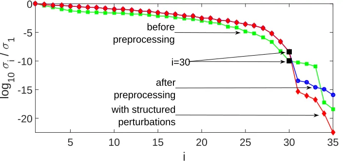
Fig. 1. The normalised singular values σi/σ1 of the Sylvester matrix of (i) f(y)
and g(y) (before preprocessing), (ii) ¯f(w) and α0g¯(w) (after preprocessing),
and (iii) ˜f(w) andβ∗
˜
g(w) (with structured perturbations), for Example 4.1. The point i= 30, which corresponds to the degree five of the GCD of ˆf(y) and ˆg(y), is marked.
Figure 1 shows the normalised singular values of the Sylvester matrix of (i) the given inexact polynomials f(y) and g(y), (ii) the polynomials ¯f(w) and α0g¯(w), which are defined in (15) and (16), and (iii) the polynomials ˜f(w) and β∗
˜
g(w), which are defined in (40) and (41). It is seen that the numerical rank of S(f, g) is 33, which is incorrect because this implies that the degree of an AGCD of f(y) and g(y) is two. The figure shows the importance of the preprocessing operations because the rank loss ofS( ¯f , α0¯g) andS( ˜f , β∗
˜ g) is 5, which is correct, and the inclusion of the structured perturbations improved the results slightly because the numerical rank is more clearly defined. The normwise relative errors in the computed coprime polynomials and AGCD in the Bernstein basis were
e(˜u(w=y/θ∗
)) = 1.25×10⁻⁶
, e(˜v(w=y/θ∗
)) = 4.86×10⁻⁸
, (60)
and
ed˜(w=y/θ∗
)= 8.07×10⁻⁷
, (61)
which are between one and three orders of magnitude larger than the relative errors inf(y) andg(y). Since θ∗
The LSE problem requires the iterative solution of (39) and Figure 2 shows the variation of the errorr(j), which is defined in (56). It is seen that convergence is achieved after a few iterations and thatr(j)≈10−15
at convergence.
iteration
5 10 15 20 25 30 35 40 45 50
log
10
error
[image:32.595.107.454.130.295.2]-14 -12 -10
Fig. 2. The error r(j) of (39) against the iteration counter j for Example 4.1.
5 10 15 20 25 30 35
−20 −15 −10 −5 0
i
log
10
σ i
/
σ 1 before
preprocessing
after preprocessing
i=30
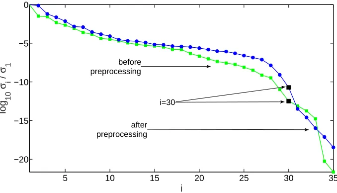
Fig. 3. The normalised singular valuesσi/σ1 of the Sylvester matrix of (i) f(y) and
g(y) (before preprocessing), and (ii) ¯f(w) and α0g¯(w) (after preprocessing),
for Example 4.1. The pointi= 30, which corresponds to the degree five of the GCD of ˆf(y) and ˆg(y), is marked.
The computations were repeated but the standard form D−1
k Tk(f, g), k =
[image:32.595.114.453.334.528.2]and the errors in the coprime polynomials and AGCD were approximately equal to the errors (60) and (61). This result shows that even if the errors of two AGCDs are approximately equal, it does not follow that the structured low rank approximations of the Sylvester matrices will also be approximately equal. Also, it is clear that significantly improved results were obtained when the modified Sylvester matrix and its subresultant matrices D−1
k Tk(f, g)Qk,
rather than the standard form D−1
k Tk(f, g) of these matrices, were used.
The coefficients of an AGCD of degree t were also computed by an approxi-mate factorisation of ¯f(w) andα0¯g(w), which is described in Section 3.2. Very similar results were obtained and the iterations in the LSE problem converged rapidly to a solution with a very small error. 2
Example 4.2 The procedure described in Example 4.1 was repeated for the polynomials,
ˆ f(y) =
16 X
i=0 ˆ ai
16 i
!
(1−y)16−i yi
= (y−0.23)4(y−0.43)3(y−0.57)3(y−0.92)3(y−1.70)3,
and
ˆ g(y) =
18 X
i=0 ˆbi 18
i !
(1−y)18−i yi
= (y−0.23)4(y−0.30)2(y−0.77)5(y−0.92)2(y−1.20)5,
except that the interval I was equal to [10−8 ,10−6
]. The method of SNTLN was applied to the perturbed polynomials after they were preprocessed, and an approximate factorisation of ¯f(w) andα0¯g(w) was computed. The relative errors in f(y) and g(y) were 5.85×10⁻⁷
and 2.18×10⁻⁷
respectively.
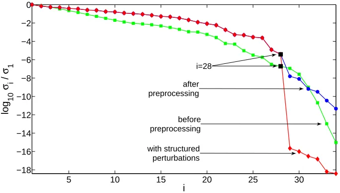
Figure 4 shows the normalised singular values of the Sylvester matrices of the pairs of polynomials (f(y), g(y)), ( ¯f(w), α0¯g(w)) and ( ˜f(w), β
∗ ˜
g(w)). The figure is similar to Figure 1 because the best result is obtained when f(y) and g(y) are preprocessed and the method of SNTLN is used to compute an AGCD. In particular, it is seen that bad results are obtained when the method of SNTLN is not applied because the numerical rank of the Sylvester matrices S(f, g) andS( ¯f , α0¯g) is not defined. By contrast, the numerical rank of S( ˜f , β∗
˜
g) is clearly defined and deg AGCD ( ˜f , β∗ ˜
g) = deg GCD ( ˆf ,ˆg) = 6.
5 10 15 20 25 30 −18
−16 −14 −12 −10 −8 −6 −4 −2 0
i
log
10
σ i
/
σ 1
after preprocessing
before preprocessing
i=28
[image:34.595.111.453.83.278.2]with structured perturbations
Fig. 4. The normalised singular valuesσi/σ1 of the Sylvester matrix of (i) f(y) and
g(y) (before preprocessing), (ii) ¯f(w) and α0g¯(w) (after preprocessing), and
(iii) ˜f(w) andβ∗
˜
g(w)(with structured perturbations), for Example 4.2. The point
i= 28, which corresponds to the degree six of the GCD of ˆf(y) and ˆg(y), is marked.
e(˜u(w=y/θ∗
)) = 1.73×10⁻⁴
, e(˜v(w=y/θ∗
)) = 1.36×10⁻⁴ ,
and
ed˜(w=y/θ∗
)= 7.97×10⁻⁴ ,
which are about three orders of magnitude larger than the relative errors in f(y) and g(y). Since θ∗
= 1.7071, this increase in errors may be due to the large condition numbers of T(f) and T(g), κ(T(f)) = 5.20× 10³ and κ(T(g)) = 1.52×10⁴ respectively, as discussed in Example 4.1.
Figure 5 shows the convergence of the iterations for the solution of the LSE problem and it is seen that it is similar to Figure 2 because good convergence is achieved very rapidly.
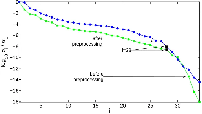
An AGCD of f(y) and g(y) was also computed when the standard form D−1
k Tk(f, g) of the Sylvester matrix and its subresultant matrices of f(y) and
g(y) was used, and the results are shown in Figure 6. This figure is similar to Figure 3 because bad results were obtained since the numerical rank of each of these matrices is not defined.
A structured low rank approximation of the Sylvester matrix of ¯f(w) and α0g¯(w) was then used to compute an AGCD of f(y) and g(y). The results were very similar to the results obtained from an approximate factorisation of
¯