White Rose Research Online URL for this paper:
http://eprints.whiterose.ac.uk/117125/
Version: Accepted Version
Article:
Ishizaka, A and Siraj, S orcid.org/0000-0002-7962-9930 (2018) Are multi-criteria
decision-making tools useful? An experimental comparative study of three methods.
European Journal of Operational Research, 264 (2). pp. 462-471. ISSN 0377-2217
https://doi.org/10.1016/j.ejor.2017.05.041
© 2017 Elsevier B.V. This manuscript version is made available under the CC-BY-NC-ND
4.0 license http://creativecommons.org/licenses/by-nc-nd/4.0/
[email protected] https://eprints.whiterose.ac.uk/ Reuse
Items deposited in White Rose Research Online are protected by copyright, with all rights reserved unless indicated otherwise. They may be downloaded and/or printed for private study, or other acts as permitted by national copyright laws. The publisher or other rights holders may allow further reproduction and re-use of the full text version. This is indicated by the licence information on the White Rose Research Online record for the item.
Takedown
If you consider content in White Rose Research Online to be in breach of UK law, please notify us by
Accepted Manuscript
Are multi-criteria decision-making tools useful? An experimental comparative study of three methods
Alessio Ishizaka , Sajid Siraj
PII: S0377-2217(17)30488-5
DOI: 10.1016/j.ejor.2017.05.041
Reference: EOR 14469
To appear in: European Journal of Operational Research
Received date: 10 February 2016 Revised date: 18 May 2017 Accepted date: 22 May 2017
Please cite this article as: Alessio Ishizaka , Sajid Siraj , Are multi-criteria decision-making tools use-ful? An experimental comparative study of three methods,European Journal of Operational Research
(2017), doi:10.1016/j.ejor.2017.05.041
A
CCE
P
T
E
D
M
A
N
U
S
CRIP
T
Highlights
• We evaluate Multi-criteria decision making tools for their usefulness
• We used incentive-based experiments
• The usefulness of different tools slightly varied but overall were found good
• Participants followed the tool s recommendation whilst revising their ranking
A
CCE
P
T
E
D
M
A
N
U
S
CRIP
T
Are multi-criteria decision-making tools useful?
An experimental comparative study of three
methods
Alessio Ishizaka1,* and Sajid Siraj2,3
¹ Portsmouth Business School, Centre for Operational Research & Logistics (CORL), University of Portsmouth, Portsmouth, PO1 3DE, United Kingdom
2 Centre for Decision Research, Leeds University Business School, Leeds, United Kingdom 3 COMSATS Institute of Information Technology, The Mall, Wah Cantonment, Pakistan
Abstract:
Many decision makers still question the usefulness of multi-criteria decision-making methods and prefer to rely on intuitive decisions. In this study we evaluated a number of multi-criteria decision-making tools for their usefulness using incentive-based experiments, which is a novel approach in operations research but common in psychology and experimental economics. In this experiment the participants were asked to compare five coffee shops to win a voucher for their best-rated shop. We found that, although the usefulness of different multi-criteria decision-making tools varied to some extent, all the tools were found to be useful in the sense that, when they decided to change their ranking, they followed the recommendation of the multi-criteria decision-making tool. Moreover, the level of inconsistency in the judgements provided had no significant effect on the usefulness of these tools.
Keywords: Decision analysis; SMART; AHP; MACBETH; Experimental evaluation.
1
Introduction
It is often the case that a single criterion is insufficient to assess a set of available alternatives. Multi-criteria decision making (MCDM) is the field of operational research wherein the decision alternatives are analysed with respect to a set of multiple (and often conflicting) criteria. Although MCDM remains an active area of research in management science (Wallenius et al., 2008), a recent survey carried out on information technology (IT) companies (Bernroider & Schmollerl, 2013) reported that 71.9% of those companies knew of the existence of MCDM
A
CCE
P
T
E
D
M
A
N
U
S
CRIP
T
methods yet only 33.3% actually used them. This gap between known and used methods is much smaller for the traditional financial methods of cost benefit and SWOT analysis that is 89.5% of companies know financial methods and 74.6% use them. Since considerable effort has been put into teaching these methods (Figueira, Greco, & Ehrgott, 2005; Ishizaka & Nemery, 2013), it is now also important to investigate the usefulness of MCDM methods and to highlight the benefits of using these methods for the actual practitioners.
According to the technology acceptance model, the intention of users to adopt new technology has two main extrinsic drivers: perceived usefulness and perceived ease-of-use (Davis, 1989; Venkatesh & Bala, 2008). One of the possible reasons that MCDM methods often remain within the academic community is that practitioners do not clearly perceive the added value (perceived usefulness). This perception/confusion of users can be linked to the following two major issues reported in the literature: 1) the methods are difficult to understand for non-experts (Giannoulis & Ishizaka, 2010) and 2) in many cases different methods do not necessarily recommend the same solution for the same problem, which adds to the confusion about which method to choose for a particular type of problem (Ishizaka & Nemery, 2013). Moreover, Bond, Carlson, and Keeney (2008) found empirically that the knowledge and values of decision makers (DMs) are under-utilized when they define their criteria for a given problem.
This situation leads us to the following two inter-connected questions: (1) Are the MCDM methods useful?
(2) Which MCDM method is more (or less) useful?
MCDM methods have been evaluated in different contexts. For example, Hülle, Kaspar, and Möller (2011) performed a bibliometric analysis to examine the use of MCDM methods in the field of management accounting and control and revealed that the Analytic Hierarchy Process (AHP) is the single most popular tool in this field. Ozernoy (1987) proposed a framework to evaluate MCDM methods and to choose the most appropriate method in a given scenario. Triantaphyllou (2000) compared several real-life MCDM issues and highlighted a number of surprising abnormalities of some of these methods Mela, Tiainen, and Heinisuo (2012) conducted a comparative analysis of MCDM techniques in the context of building design. The two main findings were that 1) different methods provide different solutions and 2) there is no single best method
A
CCE
P
T
E
D
M
A
N
U
S
CRIP
T
To give appropriate incentives, subjects were rewarded, based on their decisions, with an amount of money or goods comparable to what they could gain elsewhere.
Although the use of incentive-based experiments as a research tool has grown in management science over the years (Belot & Schröder, 2015; Corgnet, Gómez-Miñambres, & Hernán-González, 2015), the first use of these incentive-based experiments in decision analysis was performed by Ishizaka, Balkenborg, and Kaplan (2011), who experimentally validated the suitability of AHP to support decisions. However, in their study only AHP was used in a particular experiment, which has a dominating criterion that receives over 50% of the weight. Therefore, the multi-criteria nature of the problem is challengeable.
In this research we evaluated the usefulness of three decision-making techniques (AHP, SMART, and MACBETH) for a real multi-criteria problem, that is, with no dominating criteria, with incentive-based experiments. To evaluate their usefulness, their bespoke software tools were installed in a computer experimental laboratory and participants were asked to rank the five coffee shops that are available within the university campus. Three rankings were collected:
R1.From the participant at the beginning of the experiment (a priori or initial ranking) R2.From the MCDM method itself (AHP, MACBETH, or SMART) (computer-generated) R3.From the participant, a final ranking after learning the computer-generated ranking (a
posteriori ranking)
The design of the experiment is based on the study performed by Ishizaka, Balkenborg, and Kaplan (2011) with two slight modifications. Firstly, we did not ask the participants to provide a new ranking just after filling in the information on the computer and immediately before seeing the computer recommendation. This modification was made because the previous study reported that this new ranking did not differ significantly from the initial ranking (R1) of the participants. Secondly, we introduced a self-reported questionnaire at the end of the experiment to assess the perceived usefulness and ease-of-use of the three software tools. This was possible due to the fact that the length of the experiment was reduced slightly after the first modification mentioned above. These are the only differences in the design of the experiment from the previous study (apart from the differences in the MCDM methods tested and the decision problem chosen).
A
CCE
P
T
E
D
M
A
N
U
S
CRIP
T
about the order of the lower-ranked choices andto avoid the possibility that the most-preferred alternative would become overweighed. If the participant was not satisfied with the reward received, he had the possibility to exchange it for the first option of R3 by paying a small fee determined by his dissatisfaction level. These three rankings were compared statistically to determine how the decision evolved with the use of an MCDM method.
In our experimental findings, the MCDM software tools were found to be helpful and the participants were satisfied with the solutions suggested by these tools. On the feedback form, the majority of the participants perceived the usefulness of these software tools positively. Before discussing the experimental design and results, we formulate the MCDM problem below and present the necessary details about the methods used.
2
Background
Consider a finite set of discrete alternatives, , to be evaluated using a set of criteria, . Each alternative has a performance score, , with respect to the criterion . Given these performance scores, the MCDM problem is to order these alternatives from the best to the worst and in some cases also to find the overall score for each alternative. Several MCDM methods have been developed for this purpose (Figueira et al., 2005; Ishizaka & Nemery, 2013). They can be categorized broadly into three approaches (Roy, 2005; Vincke, 1992):
Approach based on synthesizing criteria: The scores for all the criteria are aggregated into a single overall score. Using such a method, a bad score for one criterion can be compensated for by a good score for another criterion. This family includes for example AHP (Saaty, 1980), MAUT (Keeney & Raiffa, 1976), SMART (Edwards, 1977), MACBETH (Bana e Costa & Vansnick, 1994), and TOPSIS (Hwang & Yoon, 1981).
Approach based on synthesizing preference relations: These methods are also called outranking methods, which permit researchers to represent indifference, strict preference, and incomparability between alternatives. The most-used methods of this family are the ELECTRE methods (for a survey see Figueira Greco Roy Słowiński ) and the PROMETHEE methods (Brans & Mareschal, 1990).
A
CCE
P
T
E
D
M
A
N
U
S
CRIP
T
programming with multiple objective functions. For example, Geoffrion, Dyer, and Feinberg (1972) and Zionts and Wallenius (1976) inferred the weights of the linear combinations of the objectives from trade-offs or pairwise judgements given by the DM for each iteration of the methods. Korhonen, Wallenius, and Zionts (1984) proposed to ask the decision maker iteratively to compare two possible alternatives until reaching the best solution by convergence. Visual interactive methods have been also developed (Korhonen, 1988). Later, other methods were developed, such as UTA (Jacquet-Lagrèze & Siskos, 1982), UTAGMS
(Greco Mousseau Słowiński ), and conjoint analysis (Green & Srinivasan, 1978). As these approaches are based on very different assumptions, they are difficult to compare with each other. In this study we focus only on the methods based on synthesizing criteria. Three methods, which have commercial supporting software tools, were selected:
1) The Simple Multi-Attribute Rating Technique (SMART) (Edwards, 1977), as implemented in Right Choice
(http://www.ventanasystems.co.uk/services/software/rightchoice/),
2) Measuring Attractiveness by a Categorical Based Evaluation Technique (MACBETH) (Bana e Costa & Vansnick, 1994), as implemented in M-MACBETH (http://www.m-macbeth.com), and
3) The Analytic Hierarchy Process (AHP) as implemented in Expert Choice (http://expertchoice.com/) (Saaty, 1977).
The three methods have different ways of capturing the evaluations of the participants and calculating the priorities. SMART asks for direct ratings on a scale from 0 to 100. MACBETH requires pairwise comparisons on an interval scale with a strict consistency check and then uses linear optimization to calculate the priorities. In AHP the DM provides pairwise comparison judgements on a ratio scale and is allowed to be inconsistent in providing these judgements. Priorities are usually calculated with the eigenvalue method. As these methods required different inputs, their interface is necessarily different. Clearly a badly designed interface would disadvantage a method. Therefore, we selected only methods that have a commercial software package, because we believe that the implementation has been studied carefully and redesigned many times (several previous versions of the software exist) by the developing companies to suit best the particular method. The interface was designed by professionals, who carefully optimized it for the underlying method. The three methods are presented in the next sub-sections.
A
CCE
P
T
E
D
M
A
N
U
S
CRIP
T
In SMART criteria and alternatives are both evaluated with a direct rating, for which the scale is usually between 0 and 100. The score of 0 implies that the alternative has no merit, while the score of 100 means that the alternative is the ideal one according to the given criterion. This rating incorporates all the criteria on the same units and therefore allows us to aggregate all these partial scores into a single score. For this aggregation the weights of the decision criteria are also acquired on the 0 to 100 scale. Once all the partial scores and criteria weights are obtained, the overall score for each alternative is calculated using the weighted sum model:
(1)
where pik is the partial score for alternative with respect to criterion and wk is the weight
of .
2.2
AHP
In AHP participants are required to give only pairwise ratio comparisons to compare either alternatives or criteria. Their focus is therefore only on two elements at a time, which should provide a more precise evaluation (Saaty, 1980, 2013). The evaluations are given on a scale from on to nine, where one represents indifference between two alternatives and nine represents extreme preference for one alternative over the other (Table 1). The comparisons are gathered in a matrix A. Local priorities or weights are calculated from the comparison matrix with the eigenvalue method:
(2)
where
A is the pairwise comparison matrix
is the priorities/weight vector
max is the maximal eigenvalue
As the comparison matrix contains redundant information, we can check whether the participant has been consistent during the exercise with the consistency index (CI), which is related to the eigenvalue method:
CI = , (3)
The consistency ratio is given by:
CR = CI/RI, (4)
A
CCE
P
T
E
D
M
A
N
U
S
CRIP
T
The random index (RI) is usually calculated as the average of the CI values generated from 500 randomly filled matrices. As a rule of thumb, it has been determined that matrices filled by a DM should not be more than 10% inconsistent compared with the RI (Saaty, 1980). Therefore, it is recommended that matrices with a CR > 0.1 are revised to decrease the inconsistency. As with the SMART method, the local priorities are aggregated using the weighted sum model to generate the final scores (si), as given in (1).
When using AHP, it is assumed that the participants are able to express their preferences on a ratio scale (given in Table 1). As this assumption is not always correct, the MACBETH method has been developed for participants who prefer interval scales.
Table 1 Pairwise ratio comparison scale for AHP
Intensity Definition
1 Equally preferable or important
2 Equally to moderately
3 Moderately more preferable or important
4 Moderately to strongly
5 Strongly more preferable or important
6 Strongly to very strongly
7 Very strongly more preferable or important
8 Very strongly to extremely
9 Extremely more preferable or important
2.3
MACBETH
In MACBETH the DM is asked to compare each pair of elements (alternatives or criteria) (xm, xn)
on an interval scale of seven semantic categories Catk, k as shown in Table 2). In the
case of hesitation, the DM is allowed to choose a range of successive categories. Table 2 Seven semantic categories
Semantic categories Cat0 Equal preference
Cat1 Very weak preference
Cat2 Weak preference
Cat3 Moderate preference
Cat4 Strong preference
Cat5 Very strong preference
Cat6 Extreme preference
Some persons prefer to evaluate ratios, while others prefer intervals. The preference depends on the
A
CCE
P
T
E
D
M
A
N
U
S
CRIP
T
The attractiveness of each element is given by solving the linear programme (Bana e Costa, De Corte, & Vansnick, 2012), where xj) is the score derived for element xj, x+ is at least as
attractive as any other element xj, and x- is at most as attractive as any other element xj:
Minimize [ (x+) (x-)]
under the constraints
(x-) = 0 (arbitrary assignment)
(xx) (xy) = 0 xx, xy Cat0
(xx) (xy) ≥ i xx, xy Cati … Cats with i,s and i ≤ s
(xx) (xy) ≥ (xw) (xz) + i s’, xx, xy Cati … Cats and xw, xz Cati …
Cats with i, s, i’, s’ , i ≤ s, i’ ≤ s’ and i > s’.
If the linear programme is infeasible, this means that the pairwise comparisons are inconsistent.
MACBETH is at first glance very similar to AHP. However, the two main differences from the user perspective are the evaluation scale (interval instead of ratio) and the need to be consistent in providing judgements. In MACBETH the priorities cannot be calculated at all when the DM is inconsistent.
We installed these software tools in our computer experimental laboratory and conducted a series of experiments to evaluate the supported methods, as discussed in the next section.
3
Description of the experiment
In our laboratory experiment, university staff and students were invited to make a straightforward but not necessarily easy choice in a real decision problem: to choose a £10 voucher for one of the coffee shops on the campus. The five coffee shops proposed were the Library Café, Park Coffee Shop, St. Andrews Café, Café Coco, and The Hub. Although there are more than five shops on the campus, these five were shortlisted due to the fact that they had no planned construction work, refurbishment, or any other activity that might have changed their properties during the experiments.
The selection criteria were explored and short-listed in a brain-storming session with ten regular users of the campus coffee shops The following six criteria were shortlisted good location product quality atmosphere waiting time space available and range of products The other criteria included opening time, price, and hospitality. The price criterion
1,2,3,4,5,6
A
CCE
P
T
E
D
M
A
N
U
S
CRIP
T
was not included due to the fact that all the shops are managed by the university catering service, which enforces the same prices across the campus. Hospitality was not considered to be important by the users, as the coffee shops are self-service. The opening and closing times were found to be similar, with a minor difference of half an hour; therefore, the opening time criterion was also not included.
Registered staff and students were invited through advertisements in different buildings, twitter broadcasts, and the university website. Participants were asked to contact us directly for booking and/or any information on the experiments. They were provided with an information sheet that included the campus map with the location of each coffee shop along with brief information about the products offered and their marketing statements.
Each participant was asked to give three sets of rankings:
1. A priori ranking (R1). Each participant was asked to rank the five coffee shops according to their own understanding and personal preferences and to write their order of ranking on the information sheet.
2. Computer ranking (R2). One of the three decision-making software tools was assigned to each participant. They were then asked to provide the required information for the algorithm to calculate a ranking. Each participant was provided with a step-wise guide to facilitate the use of the software tool.
3. A posteriori ranking (R3). After seeing the results from R2, the participants were again asked to rank the five shops, as in the first phase. This ranking was used to test whether the MCDM s advice influenced the participants priorities
After capturing the three sets of rankings, the final phase involved a payoff session. Three out of the five shops were randomly shortlisted in front of the participants. We introduced this step to encourage people to pay attention to all the assessments instead of only those related to their favourite shop. The participants were made aware of this process at the beginning of the experiment so that equal attention was given to the lower-ranked options and they had a reasonable likelihood of being selected.
Each participant was offered a £10 voucher for his most-preferred choice, which was taken from either R1 (a priori ranking) or R2 (computer-generated ranking) by tossing a coin.
A
CCE
P
T
E
D
M
A
N
U
S
CRIP
T
to sacrifice to receive the voucher of their final choice. We term this amount the willingness to swap. A random number between 0 and 1, representing the transaction fee, was generated with uniform distribution, and the voucher was swapped only if the number generated was equal to or below the willingness to swap. In this case the transaction fee was deducted from the initial £10 voucher.
This measure was used to capture the participants disagreement with either ranking R or ranking R2. For example, if the voucher was offered using R1 and the participant disagreed with a willingness to swap equal to £1, this means that the participant definitively wanted to swap his voucher, as he/she was in total disagreement with his/her original ranking (any random generated number was below or equal to 1). On the other hand, if the voucher was offered using R2 and the willingness to swap was again equal to 1, then the participant appeared to be in total disagreement with the computer-generated ranking. In the former case, the participant appeared to have changed his decision after using the software tool, supporting its usefulness. Any other amount between 0 and £1 indicated the intensity of the partial disagreement.
The experiments were scheduled as a series of one-hour sessions in computer experimental laboratories. To avoid maturation bias, each participant was restricted to evaluate only one software tool, and the participants were not allowed to reappear in subsequent sessions. The participants were asked to read the information sheet carefully and then to give their consent to participate before the start of the actual experiment.
4
Results
4.1
Participants
A
CCE
P
T
E
D
M
A
N
U
S
CRIP
T
their academic building, so it was relatively more convenient for them to participate. A total of 145 participants successfully completed the experiment. Only 1 participant did not complete the experiment due to a technical issue; specifically, the software stopped responding twice and the respondent was not willing to repeat the experiment a third time. Expert Choice (for AHP) and RightChoice (for SMART) were each evaluated by 50 participants, while M-MACBETH (for MACBETH) was evaluated by 45 participants.
Table 3 Demographic details of the participants (the numbers of participants are shown in brackets)
Software Expert Choice (50) M-MACBETH (46) RightChoice (50)
Education PhD (2), PG (6), UG (36), Staff (6) PhD (2), PG (6), UG (35), Staff (3) PhD (1), PG (4) , UG (44), Staff (1)
Nationality British (18), Bulgarian (1), Chinese (3), English (6), French (2), German (2), Greek (1), Indian (4), Italian (1), Kenyan (1), Lithuanian (1), Malaysian (1), Nigerian (1), Norwegian (1), Romanian (2), Spanish (2), Tanzanian(2)
Albanian (1), Argentinian (1), Austrian (1), British (19), Bruneian (1), English (3), Ethiopian (1), French (1), Gibraltarian (1), Greek (2), Italian (1), Japanese (1), Lithuanian (2), Nigerian (1), Romanian (4), UK (1), Zimbabwean (2)
British (28), Chinese (1), English (3), Filipino (1), German (3), Hong Kong (1), Hungarian (1), Italian (2), Malaysian (1), Polish (1), Romanian (5), Spanish (1), Swiss (1)
Gender Male (21), Female (29) Male (26), Female (20) Male (23), Female (27)
Age 24.2 (± 7.6 s.d.) 24.3 (± 8.3 s.d.) 21.5 (± 3.1 s.d.)
4.2
Criteria weight analysis
The average criteria weights captured by the three software tools are given in Table 4, along with the overall average and standard deviation. All six criteria were assigned weights of more than 12% on average, which implies that the weights were fairly distributed. The criteria of good location and product quality were found to be the two most-weighted criteria for choosing a coffee shop. Although there was no dominating criterion (having more than 50% weight), those participants who used M-MACBETH assigned a much greater weight to their top criterion that is for a good location
Table 4 Weights assigned to different criteria (mean ± standard deviation) and ANOVA results for the three tools
Criterion Expert Choice M-MACBETH RightChoice Overall F-test p
Good Location 18.5% ± 13.9 38.8% ± 17.4 20.4% ± 10.9 25.5% ± 16.8 28.76 0.000
Product Quality 25.8% ± 14.0 19.6% ± 14.1 20.5% ± 08.5 22.0% ± 12.6 3.415 0.036
Ambience 11.4% ± 09.6 12.6% ± 13.3 12.0% ± 07.4 12.0% ± 10.2 0.159 0.853
Waiting Time 13.8% ± 11.3 11.5% ± 10.5 15.1% ± 07.6 13.5% ± 09.9 1.518 0.223
Space Available 12.2% ± 08.6 07.9% ± 08.8 15.9% ± 09.8 12.1% ± 09.6 9.231 0.000
A
CCE
P
T
E
D
M
A
N
U
S
CRIP
T
The weights from the participants using Expert Choice and RightChoice are more evenly distributed and have a high rank correlation (Kendall coefficient of 0.87). The weights given by M-MACBETH have a low rank correlation with Expert Choice (Kendall coefficient of 0.33) and RightChoice (Kendall coefficient of 0.2). The ANOVA results (Table 4) for the three software tools suggest that the weights for ambience and waiting time are similar while the other four criteria have significantly different weights generated by different software tools.
The Levenes test suggested that the variances for the three groups were significantly different; however, the ANOVA test is still considered to be appropriate due to the facts that:
1) The ratio of the largest to the smallest group size is 1.08, which is considerably less than the acceptable threshold of 1.5;
2) The number of samples for all the groups is higher than 5 (as the 3 groups have sample sizes of 50, 46, and 50);
3) The ratio of the largest to the smallest variance is 1.79, which is smaller than the widely accepted threshold of 9.1.
As equal variances were not assumed, we performed the Games Howell test, which is considered to be appropriate in such conditions. The pairwise Games Howell test results are provided in Table 5 for comparing the means of the criteria weights.
Shown in bold, the weights generated by M-MACBETH were found to be significantly different from the other two methods. Each case concerns a weight calculated by M-MACBETH. Since the demographics were not significantly different for the three groups, we believe that this is due to the fact that the MACBETH technique uses a different scale for acquiring user preferences; therefore, the preference weights have different values from those obtained through AHP and SMART.
Table 5 Games Howell test to compare the means of criteria weights for the three software tools
Criterion Pairwise Comparison Mean Difference p
Good Location Expert Choice M-MACBETH -0.20314 0.000
Expert Choice RightChoice -0.01912 0.731
RightChoice M-MACBETH -0.18402 0.000
Product Quality Expert Choice M-MACBETH 0.06132 0.095
Expert Choice RightChoice 0.05285 0.070
A
CCE
P
T
E
D
M
A
N
U
S
CRIP
T
Ambience Not required
Waiting Time Not required
Space Available Expert Choice M-MACBETH 0.04299 0.051
Expert Choice RightChoice -0.03747 0.115
Right Choice M-MACBETH 0.08046 0.000 Range of
Products Expert Choice M-MACBETH 0.08838 0.001
Expert Choice RightChoice 0.02215 0.541
RightChoice M-MACBETH 0.06623 0.003
At the end of the experiment, the participants were asked to comment on the selected criteria for ranking the coffee shops. Most of the participants suggested that there was no missing criterion and that the selected criteria were helpful in the decision process. A number of participants (24 out of 146) suggested that price could have been included. We also believe that price is a very important criterion, but, as stated earlier, all the selected coffee shops are run by the university s catering service with identical prices it is therefore not important in this study
Observation 1: This is a real multi-criteria problem and not a single-criterion problem in the sense that there is no criterion with over 50% weighting on average and the least important criteria have above 12% weighting.
4.3
Alternatives score analysis
According to the computer-generated rankings, 66 (45.5%) participants selected The Hub as their most-preferred shop, while 53 (36.5%) participants considered St. Andrews Café to be the least-preferred shop. The Hub was the coffee shop that received the largest number of first rankings from all 3 software tools: 20 out of 50 by Expert Choice, 25 out of 45 by M-MACBETH, and 21 out of 50 by RightChoice. Table 6 shows the ANOVA results for the scores assigned to different shops, which suggest that the scores generated by different software tools were not significantly different. This indicates that the software tools have similar behaviour in assigning scores to the available alternatives.
Table 6 Scores assigned to the alternatives (mean ± standard deviation) with the ANOVA results
Alternatives Expert Choice M-MACBETH RightChoice Overall F-test p
Library 0.170 ± 0.104 0.207 ± 0.087 0.185 ± 0.062 0.187 ± 0.087 2.170 0.118
Park 0.213 ± 0.136 0.197 ± 0.096 0.197 ± 0.060 0.203 ± 0.102 0.397 0.673
A
CCE
P
T
E
D
M
A
N
U
S
CRIP
T
Coco 0.173 ± 0.122 0.189 ± 0.099 0.197 ± 0.057 0.187 ± 0.096 0.789 0.456
Hub 0.284 ± 0.151 0.271 ± 0.148 0.243 ± 0.057 0.266 ± 0.126 1.366 0.258
Observation 2 The alternatives scores are similar regardless of the software used
4.4
Assessing the three different rankings
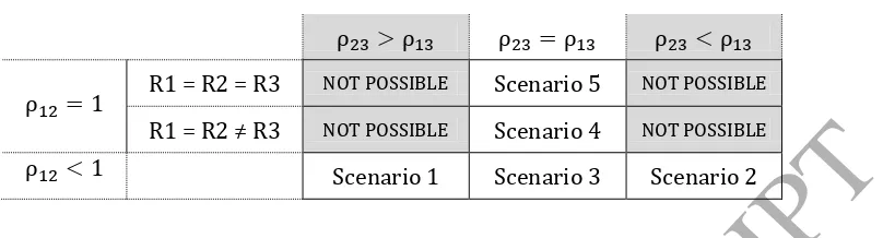
To measure the agreement between two rankings we used the Spearman s rank correlations between each pair of rankings, that is, for the correlation between R1 and R2, for the correlation between R2 and R3, and for the correlation between R1 and R3. In our experiment five scenarios involving R2 (as we were testing the usefulness of the computer ranking, a scenario without R2 would not bring any information) are plausible:
Scenario 1)
This implies that the computer-generated ranking was different from the one that was initially provided and that the computer-generated ranking was found to be closer to the finally selected one. In this case the software helped the DM in selecting his/her final choice.
Scenario 2)
This implies that the computer-generated ranking was different from the one that was initially provided but that the initial one was closer to the final set of rankings. In other words, the software was of little or no help to the DM, as it somehow suggested a ranking that was different from his/her final selection.
Scenario 3) and
This is possible when the initial and computer-generated rankings were different yet happened to be equidistant from the DM s final choice This is a situation in which it cannot be said whether the final preferences were closer to the computer-generated ones or the initial ones. However, as the software generated a different ranking, it partially helped the DM in revising his/her choices.
Scenario 4) and
This is a situation in which the software suggested the same as the a priori rankings but the final ranking was different from both. This is a strange situation, in which the ranking provided by the software does not influence the final decision but the process of using a software tool does.
Scenario 5)
A
CCE
P
T
E
D
M
A
N
U
S
CRIP
T
[image:18.595.87.491.141.250.2]DM. Regardless of whether the tool helped the DM or not, it clearly provided a way to justify his/her choices in a structured manner.
Table 7 Visualizing the five scenarios
R1 = R2 = R3 NOT POSSIBLE Scenario 5 NOT POSSIBLE R R R NOT POSSIBLE Scenario 4 NOT POSSIBLE
Scenario 1 Scenario 3 Scenario 2
The five scenarios are shown in Table 7. In our experiment, out of all these five scenarios, Scenario 1 was found to be the most frequent one. The details for each scenario are provided in Table 8. A two-tailed binomial test was carried out to gain statistical evidence on the usefulness of the three software tools. The scores for Scenarios 1, 3, and 4 were combined and categorized as successful labelled as (elped while Scenario was counted as unsuccessful labelled as Failed As discussed earlier Scenario does not provide clear support in favour of or against the software; therefore, it was excluded from this test. The results are provided in the last column of Table 8. The table shows that all three software tools were found to be useful at the significance level of 5%. The evidence obtained for RightChoice and Expert Choice were significant at the 1% level, while the evidence obtained for M-MACBETH was not found to be significant at the 1% level. The chi-squared test showed that the results for the three software tools were not significantly different ( , p = 0.837).
Table 8 The five scenarios and their frequencies of occurrence
Scenario 1 Helped
Scenario 2 Failed
Scenario 3 Helped
Scenario 4 Helped
Scenario 5 Not sure
Helped/ Failed
p
Expert Choice 24 13 6 1 6 31/13 0.006
M-MACBETH 20 13 4 1 7 25/13 0.036
RightChoice 28 12 6 2 2 36/12 0.001
Overall 73 38 16 4 14
Observation 3: The three software tools helped users in their decision making.
4.4.1
Payoff threshold exercise
A
CCE
P
T
E
D
M
A
N
U
S
CRIP
T
exchange. They exchanged the voucher straightaway by paying the penalty of £1 or by playing the game of choosing a number between 0.01 and 0.99 (see section Error! Reference source not found. for the BDM procedure).
Out of the 38 cases belonging to Scenario 2 (Table 8), in which the software did not appear to help the DM, 3 participants asked to exchange the voucher by paying the penalty of £1 straightaway. Regarding Scenario 1, 2 participants, whom the software did appear to help, asked for an exchange of vouchers; that is, they were offered their second-best choice of their final ranking but they wanted to exchange it for their first final ranked choice.
There were four cases in which participants were offered a voucher based on their initial rankings but wanted to exchange it for a certain amount (with penalties of £1, 80p, 50p, and 30p for the four cases). This implies that these participants preferred the final ranking, which was closer to the computer-generated one.
Observation 4: The disagreement with the computer-generated ranking is small.
4.4.2
Does inconsistency affect usefulness?
A
CCE
P
T
E
D
M
A
N
U
S
CRIP
T
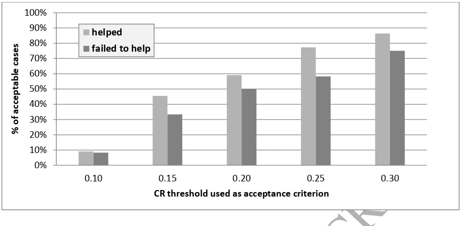
[image:20.595.58.519.64.287.2]Figure 1 Percentage of acceptable cases for using different thresholds of acceptance
Table 9 shows the frequency of participants who found the software to be helpful (Scenarios 1, 3, 4) or not (Scenario 2), grouped according to the two categories of whether their judgements were found to be acceptably consistent or not. For example, using the criterion of CR < 0.10, only 3 were marked as consistent while 31 were marked as inconsistent. On the contrary, when choosing CR < 0.3, 28 were considered to be consistent and only 6 inconsistent.
Table 9 Frequencies of consistent and inconsistent cases regarding the usefulness of Expert Choice
Threshold CR < 0.1 CR 0.1 CR < 0.15 CR 0.15 CR < 0.2 CR 0.2 CR < 0.25 CR 0.25 CR < 0.3 CR 0.3
Helped 2 20 10 12 13 9 17 5 19 3
Failed to help 1 11 4 8 6 6 7 5 9 3
= p = 0.311 0.423 0.103 0.252 0.022 0.118 0.584 0.555 0.129 0.281
After performing Yate s correction the chi-squared test for independence suggested that the helpfulness of the tools has no significant relationship with the level of inconsistency in the judgements. This is an interesting finding, as, although the use of CR has been widely debated (Bana e Costa & Vansnick, 2008; Tomashevskii, 2015), our results experimentally invalidate the threshold of CR < 0.1 and suggest a much higher threshold of acceptance.
Observation 5: AHP was helpful to the participants even with a higher level of inconsistency.
4.5
Capture of unattractive options
Out of 145 participants, 42 had visited all the shops. The other 103 participants had never been to at least 1 of the 5 coffee shops. Their judgements were based on the information provided just before the experiment as well as on some criteria that had already formulated their choice
0% 10% 20% 30% 40% 50% 60% 70% 80% 90% 100%
0.10 0.15 0.20 0.25 0.30
% o f a cc e p ta b le c a se s
CR threshold used as acceptance criterion
helped
A
CCE
P
T
E
D
M
A
N
U
S
CRIP
T
[image:21.595.86.488.127.360.2]maybe they were in another part of the campus. Table 10 provides the number of participants against the number of visited shops.
Table 10 Number of participants categorized by number of shops visited
Number of visited shops 0 1 2 3 4 5
Number of participants 1 1 7 41 53 42
Figure 2 Distribution of rankings given to the unknown shops
There were 165 such cases in which participants evaluated a shop that they had not visited (Figure 2). In 114 cases the participants ranked the unknown shop in fourth or fifth place, while the unknown shop was ranked top in only 8 cases and in second place in only 14 cases. The distribution of these rankings is shown in Figure 2, which shows that higher ranks are seldom assigned to the unknown shops. A one-way chi-squared test statistic ( ) confirmed that the distribution of rankings was not uniform and that lower ranks were assigned to the unknown shops.
Observation 6: Previous unattractive options are ranked low.
4.6
Participants feedback
At the end of the experiment, the participants were asked to provide their feedback about the tool that they had used during the experiment. Three questions were related to the perceived helpfulness, while one question was related to the perceived ease-of-use, and finally an open question provided the participants with the opportunity to give their opinion in their own words.
4.6.1
Perceived helpfulness
The participants were given the following three statements to test whether the tools were perceived to be helpful:
0 10 20 30 40 50 60 70
Ranked 1st Ranked 2nd Ranked 3rd Ranked 4th Ranked 5th
Fr
e
q
u
e
n
cy
o
f
o
cc
u
rr
e
n
A
CCE
P
T
E
D
M
A
N
U
S
CRIP
T
Q1.The computer software was helpful in ranking my choices. Q2.The software helped me in the decision-making process. Q3.I agree with the ranking suggested by the software.
The statements were scored on a Likert scale with levels ranging from strongly agree to strongly disagree with a neutral level in the middle. Positive and negative options were grouped, and a binomial test was performed. Table 11 summarizes the feedback received from the participants on these 3 questions. The results for Expert Choice and RightChoice were found to be statistically significant at the 0.05 and even the 0.01 level for all 3 questions. The participants were happy with the ranking provided by M-MACBETH, but there was not enough statistical evidence for the usefulness of M-MACBETH. In other words, although the participants agreed with the rankings generated by M-MACBETH (recall sub-section 4.4), there was not enough evidence that they also agreed on the helpfulness of this method.
Table 11 Participants feedback on the MCDM tools for the questions on usefulness
Q1
Negative Neutral Positive P Expert
Choice
5 4 41 0.000
M-MACBETH 12 7 26 0.069
RightChoice 7 2 41 0.000
Total for Q1 24 13 108
Q2
Expert Choice
9 3 38 0.000
M-MACBETH 14 6 25 0.090
RightChoice 9 3 38 0.000
Total for Q2 32 12 101
Q3
Expert Choice
8 7 35 0.002
M-MACBETH 7 7 31 0.005
RightChoice 7 7 36 0.001
Total for Q3 22 21 102
Observation 7: Expert Choice and RightChoice were perceived to be helpful, but this was not the case for M-MACBETH.
4.6.2
Perceived ease-of-use
A
CCE
P
T
E
D
M
A
N
U
S
CRIP
T
were easy to use while 7.6% remained neutral, and the remaining 25.3% disagreed with the statement.
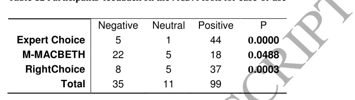
Table 12 presents the frequencies of positive, neutral, and negative feedback received for the 3
[image:23.595.141.489.210.308.2]tools and the significance level of a binomial test. All 3 software tools are under the 0.05 significance level. However, if we take a lower significance level of 0.01, M-MACBETH would not be recognized as being easy to use.
Table 12 Participants feedback on the MCDM tools for ease-of-use
Negative Neutral Positive P
Expert Choice 5 1 44 0.0000
M-MACBETH 22 5 18 0.0488
RightChoice 8 5 37 0.0003
Total 35 11 99
Observation 8: Expert Choice and RightChoice were perceived as being easy to use, but this was less the case for M-MACBETH.
4.6.3
Qualitative feedback
The participants were asked to comment on their experience with the tool that they had used. The feedback collected was then transcribed electronically to perform sentiment analysis using the Stanford Sentiment Tree Bank (nlp.stanford.edu). The results are shown in Table 13, in which the phrases are classified as carrying either positive or negative sentiments. For example, phrases like easy to use and it helped carry a positive sentiment while some other phrases such as a bit confusing and was too complicated convey a negative sentiment Some of the statements were declared as neutral, as it was hard to declare them as either positive or negative.
Table 13 Textual analysis of the qualitative feedback
Expert Choice M-MACBETH RightChoice
Positive terms
easy to use; yes helpful; it helped; it was
really helpful; software was helpful; user
friendly; was helpful; yes it was
21 11 17
Neutral terms
a bit; not sure; yes but
2 2 3
Negative terms
a bit confusing; could be streamlined; difficult
A
CCE
P
T
E
D
M
A
N
U
S
CRIP
T
to use; hard to; it would have been; overly
complicated; too complicated; was confusing;
was too complicated
p 0.00 0.28 0.024
As shown in Table 13, 49 positive phrases were detected against 21 negative ones. The positive perception of the 3 software tools is statistically significant with a binomial 2-tail test (p = 0.001). When considering each software tool individually, the evidence of positive feedback for Expert Choice and RightChoice was supported with p = 0.00 and 0.024, respectively, at the significance level of 0.05, as recommended by Craparo (2007). However, the statistical test for MACBETH failed with p = 0.28. The feedback for Expert Choice contained the highest number of positive comments, while M-MACBETH received the highest number of negative phrases in the participants feedback RightChoice was also found to have a positive-dominated response, that is, 17 positive and only 6 negative phrases.
Observation 9: The feedback on the MCDM tools contained more words bearing positive sentiments than negative sentiments.
5
Conclusion
A
CCE
P
T
E
D
M
A
N
U
S
CRIP
T
techniques. After investigating the question of usefulness and obtaining positive results, the challenge is to communicate these benefits and usefulness to the actual practitioners.
5.1
Limitations and future work
One of the major limitations of this work is that we applied our analysis to only one specific decision problem; therefore, it needs to be tested for different types of problems in different contexts so that the results can be generalized. In future works we plan to apply our experimental approach to other families of multi-criteria methods and to other decision problems.
As introduced earlier, different software tools come with different user interfaces due to the different inputs required and hence provide different user experiences. Therefore, it is not possible to separate the perception of helpfulness regarding the method itself and the perception of helpfulness of the software interface. Ideally, participants should be offered a uniform user interface across these methods. Future research should develop a uniform interface, although the inputs required would be different.
Future experiments could also include placebo software in which rankings are generated randomly without any analysis. This study would aim to test the hypothesis that participants trust computer-generated recommendations blindly and therefore would adopt any recommendation. However, additional care would be required due to the involvement of deception. Finally, the analysis could also be enriched further by conducting an additional satisfaction survey after participants have spent their voucher in the coffee shop.
Acknowledgement
We are thankful to the Portsmouth Business School for providing adequate funding and facilities to conduct this research under the Research Project Fund (RPF) scheme.
References
Bana e Costa, C., De Corte, J.-M., & Vansnick, J.-C. (2012). MACBETH. International Journal of Information Technology & Decision Making, 11, 359 387.
A
CCE
P
T
E
D
M
A
N
U
S
CRIP
T
Bana e Costa, C., & Vansnick, J. (2008). A critical analysis of the eigenvalue method used to derive priorities in AHP. European Journal of Operational Research, 187, 1422 1428.
Becker, G. M., Degroot, M. H., & Marschak, J. (1964). Measuring utility by a single-response sequential method. Behavioral Science, 9, 226 232.
Belot, M., & Schröder, M. (2015). The spillover effects of monitoring: A field experiment.
Management Science, online advance publication, doi.org/10.1287/mnsc.2014.2089.
Bernroider, E. W. N., & Schmollerl, P. (2013). A technological, organisational, and environmental analysis of decision making methodologies and satisfaction in the context of IT induced business transformations. European Journal of Operational Research, 224, 141 153.
Bond, S., Carlson, K., & Keeney, R. (2008). Generating objectives: Can decision makers articulate what they want? Management Sciences, 54, 56 70.
Brans, J., & Mareschal, B. (1990). The PROMETHEE methods for MCDM; The PROMALC, GAIA and BANKADVISER software. In C. Bana e Costa (Ed.), Readings in multiple criteria decision aid
(pp. 216 252). Berlin: Springer-Verlag.
Cao, D., Leung, L. C., & Law, J. S. (2008). Modifying inconsistent comparison matrix in analytic hierarchy process: A heuristic approach. Decision Support Systems, 44, 944 953.
Corgnet, B., Gómez-Miñambres, J., & Hernán-González, R. (2015). Goal setting and monetary incentives: When large stakes are not enough. Management Science, advance online publication, doi.org/10.1287/mnsc.2014.2068.
Craparo, R. (2007). Significance level. In N. Salkind (Ed.), Encyclopedia of measurement and statistics (Vol. 3, pp. 889 891). Thousand Oaks: SAGE Publications.
Davis, F. D. (1989). Perceived usefulness, perceived ease of use, and user acceptance of information technology. MIS Quarterly, 13, 319 340.
Edwards, W. (1977). How to use multiattribute utility measurement for social decisionmaking.
IEEE Transactions on Systems, Man and Cybernetics, 7, 326 340.
Figueira, J., Greco, S., & Ehrgott, M. (2005). Multiple criteria decision analysis: State of the art surveys. New York: Springer.
A
CCE
P
T
E
D
M
A
N
U
S
CRIP
T
Geoffrion, A., Dyer, J., & Feinberg, A. (1972). An interactive approach for multi-criterion optimization, with an application to the operation of an academic department. Management Science, 19, 357 368.
Giannoulis, C., & Ishizaka, A. (2010). A web-based decision support system with ELECTRE III for a personalised ranking of British universities. Decision Support Systems, 48, 488 497.
Greco S Mousseau V Słowiński R Ordinal regression revisited Multiple criteria ranking using a set of additive value functions. European Journal of Operational Research, 191, 416 436.
Green, P., & Srinivasan, V. (1978). Conjoint analysis in consumer research: Issues and outlook.
Journal of Consumer Research, 5, 103 123.
Hülle, J., Kaspar R., & Möller, K. (2011). Multiple criteria decision-making in management accounting and control State of the art and research perspectives based on a bibliometric study. Journal of Multi-Criteria Decision Analysis, 18, 253 265.
Hwang, C.-L., & Yoon, K. (1981). Multiple attribute decision making: Methods and applications. New York: Springer-Verlag.
Ishizaka, A., Balkenborg, D., & Kaplan, T. (2011). Does AHP help us make a choice? Journal of the Operational Research Society, 62, 1801 1812.
Ishizaka, A., & Nemery, P. (2013). Multi-criteria decision analysis. Chichester, UK: John Wiley & Sons Inc.
Jacquet-Lagrèze, E., & Siskos, J. (1982). Assessing a set of additive utility functions for multicriteria decision-making, the UTA method. European Journal of Operational Research, 10, 151 164.
Keeney, R., & Raiffa, H. (1976). Decision with multiple objectives: Preferences and value tradeoffs. New York: Wiley.
Korhonen, P. (1988). A visual reference direction approach to solving discrete multiple criteria problems. European Journal of Operational Research, 34, 152 159.
Korhonen, P., Wallenius, J., & Zionts, S. (1984). Solving the discrete multiple criteria problem using convex cones. Management Science, 30(11), 1336 1345.
A
CCE
P
T
E
D
M
A
N
U
S
CRIP
T
Ozernoy, V. (1987). A framework for choosing the most appropriate discrete alternative multiple criteria decision-making method in decision support systems and expert systems.
Lecture Notes in Economics and Mathematical Systems, 56 64.
Roy, B. (2005). Paradigms and challenges. In S. Greco, M. Ehrgott, & J. R. Figueira (Eds.), Multiple criteria decision analysis: State of the art surveys (pp. 3 24). New York: Springer-Verlag.
Saaty, T. (1977). A scaling method for priorities in hierarchical structures. Journal of Mathematical Psychology, 15, 234 281.
Saaty, T. (1980). The analytic hierarchy process. New York: McGraw-Hill.
Saaty, T. (2013). The modern science of multicriteria decision making and its practical applications: The AHP/ANP approach. Operations Research, 61, 1101 1118.
Tomashevskii, L. (2015). Eigenvector ranking method as a measuring tool: Formulas for errors.
European Journal of Operational Research, 240, 774 780.
Triantaphyllou, E. (2000). Multi-criteria decision making methods: A comparative study. US: Springer.
Venkatesh, V., & Bala, H. (2008). Technology acceptance model 3 and a research agenda on interventions. Decision Sciences, 39, 273 315.
Vincke, F. (1992). Multicriteria decision-aid. Wiley, Chichester.
Wallenius, J., Dyer, J., Fishburn, P., Steuer, R., Zionts, S., & Deb, K. (2008). Multiple criteria decision making, multiattribute utility theory: Recent accomplishments and what lies ahead.
Management Science, 54, 1336 1349.
Xu, Z., & Wei, C. (1999). A consistency improving method in the analytic hierarchy process.
European Journal of Operational Research, 116, 443 449.