Blind Thrusting, Surface Folding, and the Development
of Geological Structure in the
M
w
6.3 2015
Pishan (China) Earthquake
E. A. Ainscoe1 , J. R. Elliott1,2 , A. Copley3, T. J. Craig2 , T. Li4 ,
B. E. Parsons1, and R. T. Walker1
1COMET, Department of Earth Sciences, University of Oxford, Oxford, UK,2COMET, School of Earth and Environment,
University of Leeds, Leeds, UK,3COMET, Bullard Labs, Department of Earth Sciences, University of Cambridge, Cambridge,
UK,4School of Earth Science and Engineering, Sun Yat-Sen University, Guangzhou, China
Abstract
The relationship between individual earthquakes and the longer-term growth of topography and of geological structures is not fully understood, but is key to our ability to make use of topographic and geological data sets in the contexts of seismic hazard and wider-scale tectonics. Here we investigate those relationships at an active fold-and-thrust belt in the southwest Tarim Basin, Central Asia. We use seismic waveforms and interferometric synthetic aperture radar (InSAR) to determine the fault parameters and slip distribution of the 2015Mw6.3Pishan earthquake—a blind, reverse-faulting event dipping toward the Tibetan Plateau. Our earthquake mechanism and location correspond closely to a fault mapped independently by seismic reflection, indicating that the earthquake was on a preexisting ramp fault over a depth range of∼9–13 km. However, the geometry of folding in the overlying fluvial terraces cannot be fully explained by repeated coseismic slip in events such as the 2015 earthquake nor by the early postseismic motion shown in our interferograms; a key role in growth of the topography must be played by other mechanisms. The earthquake occurred at the Tarim-Tibet boundary, with the unusually low dip of 21∘. We use our source models from Pishan and a 2012 event to argue that the Tarim Basin crust deforms only by brittle failure on faults whose effective coefficient of friction is≤0.05±0.025. In contrast, most of the Tibetan crust undergoes ductile deformation, with a viscosity of order 1020–1022Pa s. This contrast in rheologies provides an explanation for the low dip of the earthquake fault plane.1. Introduction
The relationship between individual earthquake cycles and the long-term development of fold and thrust structures is not fully understood. Theoretical geometrical models have been proposed to describe how folds form and grow over time above thrust faults with various geometries (e.g., Erslev, 1991; Homza & Wallace, 1995; Suppe, 1983; Suppe & Medwedeff, 1990), and the development of thrust-related folds in nature over tens of thousands to millions of years has been studied by analysis of drainage, topography and structural geology (e.g., Burbank et al., 1999; Daëron et al., 2007). However, it is not clear how complex fault and fold structures develop through repeated earthquake cycles nor how these longer-term structures may or may not correlate with the surface deformation measured today (e.g., Nissen et al., 2007). The relative importance of interseismic, coseismic, and postseismic deformation to the development of geological structures and topog-raphy in regions of continental shortening is not known. Given that historical records of earthquakes are often much shorter than recurrence times for each fault, data sources with longer temporal coverage and global spatial coverage, such as digital elevation models and geomorphology, combined with dating, provide a valu-able opportunity to augment assessments of seismic hazard (Stein & King, 1984; Taylor & Yin, 2009; Zhou et al., 2015; Talebian et al., 2016). Making use of this opportunity depends on developing an ability to interpret the spatial and temporal relationship between long-term structures and individual earthquakes. To address this issue, here we investigate structural growth at a blind range front thrust where we can directly compare sur-face motion observations from interferometric synthetic aperture radar (InSAR), subsursur-face seismic reflection data and surface geomorphology.
In addition, the Pishan earthquake represents an opportunity to investigate the wider question of what con-trols the geometry of active fault planes. By examining the material properties and behavior of the lithosphere
RESEARCH ARTICLE
10.1002/2017JB014268
Key Points:
• Coseismic fault geometry and location closely match a preexisting blind fault
• Quaternary fold grows by distributed deformation in the overlying sediments and does not align with coseismic or early postseismic uplift • Rheology contrast between the Tarim
Basin and Tibet may explain the earthquake’s low dip angle
Supporting Information:
• Supporting Information S1
Correspondence to:
E. A. Ainscoe,
eleanor.ainscoe@earth.ox.ac.uk
Citation:
Ainscoe, E. A., Elliott, J. R., Copley, A., Craig, T. J., Li, T., Parsons, B. E., & Walker, R. T. (2017). Blind thrusting, surface folding, and the development of geological structure in the Mw6.3 2015 Pishan (China) earthquake.Journal of Geophysical Research: Solid Earth,122, 9359–9382. https://doi.org/10.1002/2017JB014268
Received 31 MAR 2017 Accepted 19 OCT 2017
Accepted article online 24 OCT 2017 Published online 27 NOV 2017
Figure 1.(a) Overview map of the Tarim Basin and its surroundings. ATF: Altyn Tagh Fault. KKF: Karakax Fault. BU: Bachu Uplift. Kg: Kashgar city. Black rectangle shows the area of Figure 1b. (b) Landsat 8 imagery (RGB 654) of the southwest Tarim Basin region. Faults after Avouac and Peltzer (1993) and Wei et al. (2013). (c) Landsat imagery around the epicenter of the 2015 Pishan earthquake (red star) and showing the incised area above the Hotan Fold and Thrust Belt (HFT). A-B-C shows the location of the seismic reflection profile (section 4).
beneath the Tarim Basin and Tibetan Plateau we are able to examine how the contrast between them affects the geometry of the resulting faulting.
On 3 July 2015 anMw6.3earthquake hit Pishan county in Xinjiang, China, at 01:07:47 UTC (09:07 local time). Local media reported three deaths and damage to several thousand buildings. The epicenter was located approximately 20 km southwest of the historic Silk Road town of Pishan (also known as Guma), an oasis town on the edge of the Taklamakan Desert. Thirty aftershocks with magnitudemb ≥ 4.0were reported by the United States Geological Survey (USGS) in the 7 months following the earthquake and form a distributed pattern roughly trending northwest-southeast, approximately 100 km in extent (Figure 1).
interferograms covering the first 7 months following the event. We correlate the relative locations and mag-nitudes of coseismic and postseismic displacements to the tectonic geomorphology of the area in order to constrain the mechanism by which the current topography has formed over the late Quaternary. We compare our results to a seismic reflection survey across the same location to investigate the full history of the underly-ing folds and thrusts in the Pliocene. Placunderly-ing our results in a wider regional context, we use our source models for the Pishan earthquake and a smaller 2012 event 350 km to the northeast in the central Tarim Basin to con-strain the rheology of components in the surrounding Tarim-Tibet collision zone and examine the effect they had on the geometry of the faulting at Pishan.
2. Tectonic Setting
Pishan is situated at the margin between the Tibetan Plateau and the southwestern corner of the Tarim Basin, 800 km north of the Himalayan front (Figure 1). The Tarim Basin acts as a rigid block within the India-Eurasia collision; although it is surrounded by mountain ranges undergoing active shortening—the Tien Shan to the north, the Pamir mountains to the west, and the Tibetan Plateau to the south—the Tarim Basin has low seismicity, flat topography, and GPS measurements show little internal deformation (England & Molnar, 2005; Molnar & Tapponnier, 1978). At the southwest corner of the Tarim Basin, where we focus our attention in this paper, gravity anomalies (Lyon-Caen & Molnar, 1984), receiver functions (Kao et al., 2001; Wittlinger et al., 2004), seismic refraction (Qiusheng et al., 2002), and geological mapping (Matte et al., 1996) show that the Tarim Basin is underthrusting the Western Kunlun Mountains, which form the edge of the Tibetan Plateau. GPS stations are relatively sparse, but 0–3 mm/yr of N-S convergence is possible within the uncertainties of the measurements (Ge et al., 2015) and the region has hostedMs7.0 and 6.8 earthquakes in 1882 and 1902, respectively, and anMw6.1 event in 1956 (Avouac & Peltzer, 1993; Lee et al., 1978; Li et al., 2012; United States Geological Survey, 2017) (Figure 1).
Across the northern range front of the Western Kunlun Mountains the elevation changes rapidly from 5,000 m to 2,100 m within a horizontal distance of just 50 km, and post-Mesozoic basin sediments have a thickness of around 10 km (Jiang & Li, 2014; Wei et al., 2013). The most basinward active shortening visible at the surface is in the low-lying, gently northward sloping piedmont. The structures here are known as the Hotan Fold and Thrust Belt and are expressed around Pishan as a belt of exposed and folded bedrock and terraces crossing from 77.0∘E, 37.75∘N to 78.75∘E, 37.2∘N (Figure 1). The total upper crustal shortening across the Hotan Fold and Thrust Belt has been of the order of several tens of kilometers (Jiang et al., 2013) and occurred in two stages, the first∼23–10 Ma and the present stage, into which the 2015 Pishan earthquake falls and which began∼5 Ma (Jiang & Li, 2014; Wei et al., 2013).
3. The 3 July Pishan Earthquake Fault Geometry and Coseismic Slip Distribution
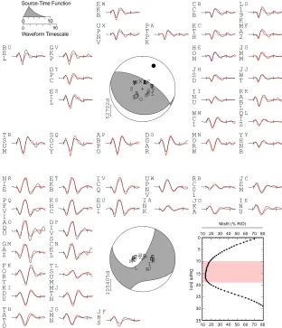
3.1. Body Waveform ModelingWe performed a joint inversion of teleseismicPandSHwaveforms to obtain the focal parameters and source time function of the Pishan mainshock. Seismograms (25 forP, 23 forSH) from stations at epicentral distances of 30–80∘were band-pass filtered to 15–100 s and converted to the response of a WWSSN long-period seis-mometer. These were then inverted using the MT5 program of Zwick et al. (1994) (based on the algorithm of McCaffrey & Abers, 1988; McCaffrey et al., 1991). The method is well established and described elsewhere (e.g., Craig et al., 2011; Molnar & Lyon-Caen, 1989; Sloan et al., 2011). Stations were weighted to account for the uneven distribution of their azimuths, andPseismograms were given double the weight ofSHseismograms to address the amplitude imbalance. The velocity structure at the source was specified as a simple half-space velocity model, withVp =6.00km/s,Vs =3.45km/s. While this is likely to be fast relative to the uppermost crustal layers, it represents a good average for the bulk crustal properties, and at the frequency range used, the waveforms are not sensitive to short-length scale variations in the shallow velocity structure.
Table 1
Pishan Mainshock Fault Parameters From Catalogs, Body Wave Modeling, and Uniform Slip Inversion of InSAR
Long. Lat. Strike Dip Rake Centroid depth Length Width Slip Mo
Model (deg) (deg) (deg) (deg) (deg) (km) (km) (km) (m) (1018Nm) M w
GCMT 78.14b 37.58b 109 22 85 15.6 - - - 5.3 6.4
Auxiliary plane 294 68 92
USGS NEIC 78.154c 37.459c 105 24 60 15.5 - - - 5.3 6.4
Auxiliary plane 317 69 102
He et al. (2016)a 78.1390b 37.7157b 113.8 27.2 93.7 10.98 22.18 8 0.6 4.12 6.33
±0.0004 ±0.0005 ±0.2 ±0.2 ±0.6 ±0.05 ±0.05
Wen et al. (2016)a 78.057d 37.571d 114.0 23.6 92.6 8.8 22.1 10.1 0.59 - 6.4 ±0.4 km ±0.3 km ±1.6 ±1.5 ±3.2 ±0.4 ±0.5 ±1.0 ±0.06
Body wave (this study) 78.14e 37.58e 102 23 73 16.5 - - - 2.5 6.2
Auxiliary plane 300 68 97
InSAR (this study)a 78.140f 37.777f 112 21 83 11.0 21.5 9.3 0.6 4.0 6.3 ±1.7 km ±2.7 km ±2.4 ±2.5 ±4.9 ±0.8 ±1.1 ±2.1 ±0.2 ±0.2
aUniform slip model.bCentroid.cEpicenter. Focal depth 20.0 km.dNot specified. eFixed at GCMT location.fUpdip projection of center.
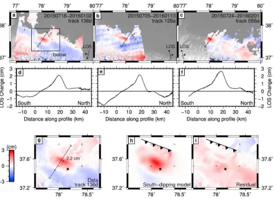
[image:4.612.217.529.312.675.2]Figure 3.Coseismic interferograms from three Sentinel-1 tracks. (top row) The full extent of each interferogram used in this study, overlaid on a hillshaded topographic map. The lobe with the greatest change shows decreased range, that is, displacement toward the satellite. The time span of each interferogram is printed on the right, format yyyymmdd. Black box shows the area enlarged in Figure 3 (bottom row). Black stars show epicenter (USGS), P marks Pishan town.
3.2. InSAR
3.2.1. Coseismic Sentinel-1 Interferograms
We used InSAR data showing ground displacements to add an independent estimate of the earthquake cen-troid parameters and made use of the interferograms’ dense near-field spatial coverage to constrain the fault location, slip extent, and slip distribution. The coseismic ground deformation was measured by construct-ing interferograms usconstruct-ing data from the European Space Agency’s (ESA) Sentinel-1A satellite, which carries a C-band synthetic aperture radar (SAR). We made interferograms from three tracks: two ascending and one descending (Figure 3 and Table 2), each had a time span of 24 days.
We processed the single look complex (SLC) images using the GAMMA software, following the method detailed in Appendix A. The final interferograms were geocoded and downsampled to 100 m. They show a simple two-lobed signal that varies smoothly over∼45 km, consistent with a blind event associated with buried faulting (Figure 3). The northern lobe indicates motion toward the satellite, with a peak line-of-sight (LOS) displacement of 11.8 cm for track 056a. The southern lobe represents motion away from the satellite,
Table 2
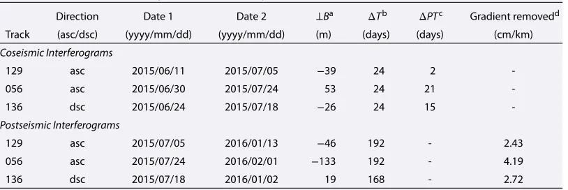
Details of the Sentinel-1A Interferograms Used in This Study
Direction Date 1 Date 2 ⊥Ba ΔTb ΔPTc Gradient removedd
Track (asc/dsc) (yyyy/mm/dd) (yyyy/mm/dd) (m) (days) (days) (cm/km)
Coseismic Interferograms
129 asc 2015/06/11 2015/07/05 −39 24 2
-056 asc 2015/06/30 2015/07/24 53 24 21
-136 dsc 2015/06/24 2015/07/18 −26 24 15
-Postseismic Interferograms
129 asc 2015/07/05 2016/01/13 −46 192 - 2.43 056 asc 2015/07/24 2016/02/01 −133 192 - 4.19 136 dsc 2015/07/18 2016/01/02 19 168 - 2.72
aPerpendicular baseline at scene center.bTime span.cPostseismic interval.dTopographically correlated phase gradient
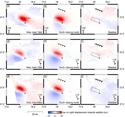
[image:5.612.173.580.579.715.2]Figure 4.Results of uniform-slip models for the coseismic interferograms. (a) Unwrapped interferogram for track 136, location of maximum line-of-sight displacement toward the satellite of 11.4 cm is marked by the black dot. (b, c) Model and residual line-of-sight displacement for a south dipping fault model. Blacked ticked lines: updip projection of the fault plane to the surface. Black boxes: location of the uniform slip patch at depth. Black stars: epicenter (USGS). The equivalent figures for tracks (d–f ) 129 and (g–i) 056.
with peak LOS motion of 5.9 cm for the same track. The three tracks cover the spatial extent of the entire defor-mation zone, although coherence is lost in some areas of the desert 50 km to the north of Pishan. While the two ascending interferograms covering the earthquake have the same look geometry, the different locations of the peak displacement of the earthquake relative to the SAR scene extents provides differing sensitivities to the ground deformation: the earthquake lies in the near-range portion of track 056a, with incidence angles
∼30∘, indicating a greater sensitivity to vertical motion than east-west; for track 129a the incidence angle is nearer 45∘in the far range, resulting in an equal sensitivity to vertical and east-west ground displacement. 3.2.2. Uniform-Slip Model
Table 3
Misfits Between our Models and Interferograms
Track RMS (cm) Overall RMS Period Dip direction Uniform/Distributed 129 056 136 (cm) Coseismic South Distributed 0.58 0.61 0.52 0.57
South Uniform 0.59 0.66 0.53 0.60
Postseismic South Distributed 0.38 0.30 0.37 0.36
3.2.3. Distribution of Coseismic Slip
To enable a more detailed comparison between coseismic slip and the long-term geological structure visible in seismic reflection profiles (section 4), we invert for the distribution of slip on the fault plane based upon the geometry found in section 3.2.2.
Taking the location, strike, dip, and rake from the uniform slip inversion, we extended the fault plane later-ally, to 20 km depth and to the surface. The fault was split into patches of size 2 km in length and∼2 km in downdip width, and we carried out a nonnegative least squares inversion to solve for slip on each patch and for the interferogram nuisance parameters (Funning et al., 2005; Wright et al., 2004). In order to find a physi-cally realistic solution, the method imposes a positivity constraint and Laplacian smoothing. The multiplying factor of the Laplacian (i.e., the strength of the smoothing) determines the balance between roughness and root-mean-square (RMS) misfit to the downsampled InSAR data. We chose a smoothing factor in the apex of the RMS misfit versus roughness curve, aiming to give the highest resolution possible without introducing spurious slip patches (Figure S1 in the supporting information). By inspection of the results from a variety of smoothing factors, we see that our main conclusions are not strongly influenced by the choice of smoothing factor from within a reasonable range.
Our preferred slip distribution is shown in Figure 5. It shows a single slip patch with a peak slip of 1.1 m, length of∼20 km, and downdip width of∼10 km. This model corresponds to the majority of the slip being at 9.5–13 km depth. We found no substantial slip above 8 km depth. Our interferograms have good coverage above the surface projection of the fault planes, and we can be confident in our conclusion that the earth-quake was blind. Our results are consistent with field observations that found no evidence of surface ruptures (Lu et al., 2016) and are also consistent with our interpretation of local geomorphology (section 5), with seismic reflection profiles (Li et al., 2016) and the slip distributions of Zhang et al. (2016) and Sun et al. (2016) but contradict earlier InSAR-derived slip distributions by Wen et al. (2016) and He et al. (2016). The latter slip distributions each show∼20 cm of slip in the shallow portion of the fault plane, including at the surface.
[image:7.612.204.544.515.696.2]Figure 6.Seismic reflection profile along the line A-B-C (Figure 1) (adapted from Li et al. (2016) and with our modified velocity model). (top) Uninterpreted. (bottom) With interpretation. The back thrust at 10 km horizontal distance is our interpretation, all other interpretation is taken from Li et al. (2016). Dashed black lines: fault planes found by our uniform slip models. H’ and H: fold axes. N2-Q: Pliocene-Quaternary 3.6 Ma to present (Zheng et al., 2000). N2: Pliocene. N1: Miocene. E: Paleogene. Pz-Mz: Paleozoic-Mesozoic. Pre-Pz: Precambrian. (left) Colored squares show the depth distribution of moment release per unit depth in our finite slip model.
Our interferograms show that there is no discontinuity at the surface projection of the fault, and we suggest that the shallow slip suggested by other studies (He et al., 2016; Wen et al., 2016) is an artifact as a conse-quence of their incomplete data coverage in the Taklamakan Desert (Figure 1) above the surface projection of the fault plane—the area most sensitive to shallow slip.
4. Comparison of Fault Positions Derived From InSAR and Seismic Reflection
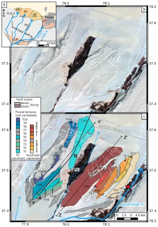
Figure 7.(a) Simplified sketch map of the geomorphology around the Pishan terraces. UF: fan upstream of the fold. DF: downstream fans. (b) Uninterpreted SPOT7 imagery of the Pishan terraces and surface scarps. A 1.5 m resolution panchromatic imagery has been used to pansharpen 6 m resolution multispectral (RGB) imagery. (c) Interpreted version of the same area. Colored polygons: terraces with profiles in Figure 8. Solid black lines: profiles Y-Y’ and Z-Z’, distance markers at 0 km. Red star: epicenter (USGS). Px: Pinxinaxiang town. Thick blue arrow: active river. Thin blue arrows: inactive drainage routes. Line A-B: part of the seismic reflection line shown in Figure 1. Grayed-out terraces were not used in Figure 8.
by Li et al. (2016). The back thrust is the most prominent sign of internal deformation within the wedge and offsets a prominent horizon at 10 km horizontal distance. It is not enough alone to account for the wedge thickening, but it could contribute to keeping the reflectors above it subhorizontal; if the back thrust slipped 1 m for every 2.2 m of slip on the frontal ramp, then the two faults would have equal throw. The back thrust is in the hanging wall of the ramp and presumably is transported by it. Due to the constant thickness of the Pliocene unit (N2 on Figure 6), Li et al. (2016) label it as pregrowth stratum and conclude that the initiation age of the deformation of the wedge is≤3.6 Ma.
Li et al. (2016) used a first-approximation velocity model: a uniform velocity of 3,000 m/s. While 3,000 m/s is appropriate for the Cenozoic section, it is likely to be an underestimate for the deeper units. The Paleozoic and Mesozoic units are predominantly sediments, such as limestones, dolomite, and gypseous mudstone, whereas the pre-Paleozoic units consist of metamorphic and volcanic rocks (Lu et al., 2016). Data from Kashgar, where the lithologies are thought to be similar to the Pishan area, indicate that the velocity of the pre-Cenozoic units is commonly in the range∼4,500–5,500 m/s, whereas the Cenozoic unit is usually∼2,800–3,200 m/s (Heermance et al., 2008). We have therefore updated the seismic reflection profile, changing the time-depth conversion to incorporate a velocity model of 3,000 m/s for the Cenozoic sediments and 5,000 m/s for ear-lier units. The result is shown in Figure 6, and the location of the profile is shown in Figure 7. The top four units (N2-Q to E) of the newly converted profile are unchanged from the original, but below that, the effect is that reflections have been deepened, with the greatest effect on the deepest parts of the profile. The Precambrian-Paleozoic unit boundary level with the zero kilometer horizontal distance marker on Figure 6 has increased in depth from 10.5 km to 12 km and the dip of the front ramp fault has increased from 10–14∘ (Li et al., 2016) to 16–20∘, bringing the dip into line with teleseismic and InSAR estimates for the 2015 earthquake (Table 1).
The southward dipping InSAR solution matches the independently constructed updated seismic reflection profile closely in depth, location, and dip. We note that, as always, both the InSAR fault location and geometry and the reflection profile have uncertainties associated with them and it would be unwise to rely on inter-preting the fine details of the comparison. However, the excellent match is strong evidence that the causative fault of the Pishan earthquake was the frontal wedge thrust that is visible in the reflection profile (Li et al., 2016). This consistency indicates that InSAR solutions of active faulting could provide useful constraints on the velocity migration of seismic reflection profiles, particularly in areas of thick sedimentary cover lacking borehole constraints on seismic velocities.
5. Folding in the Geomorphology
5.1. Fluvial Terrace DeformationThe Pishan earthquake occurred under the alluvial apron that skirts the southern edge of the Taklamakan Desert. Drainage runs to the north-northeast from the Western Kunlun Mountains. A belt of incision∼25 km wide crosses from northwest to southeast parallel to the strike of the fault (Figure 1, section 2). In some places it exposes pre-Quaternary sediments (Li et al., 2016; Matte et al., 1996), and in the Pishan area it preserves a sequence of folded fluvial terraces. The mainshock epicenter and the surface-projected fault plane lie in this terraced area (Figures 1 and 5b).
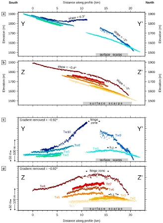
We mapped the terraces adjacent to the Kuoshtagh and Pinxinaxiang town rivers using 1.5 m resolution SPOT7 optical imagery, the 30 m SRTM1 DEM, GoogleEarth, and Bing Maps (Figure 7). We inferred relative age from mapping, surface preservation, and height and labeled the terraces in order of increasing age but were not able to correlate terraces between the two catchments (i.e., Te1 does not necessarily correlate with Tw1). Topographic profiles projected onto lines Y-Y’ and Z-Z’ are shown in Figure 8. In order to isolate the tectonic contribution to topography, it is necessary to remove the depositional slope. We have assumed and removed a linear depositional gradient of 0.92∘as described in the next paragraph. After the removal of this depositional gradient, we assume that any remaining elevation changes on individual terraces are due to postdepositional tectonic deformation (e.g., Molnar et al., 1994; Poisson & Avouac, 2004; Walker et al., 2015).
Quantification of the original depositional gradient is not straightforward. Upstream, a single river forms one broad fan as it leaves the mountains (UF on Figure 7a), but through the incised belt drainage has been split into four channels, each of which has formed its own small fan downstream of the terraces (DF on Figure 7a). This prevents us from following coeval depositional surfaces upstream and downstream of the deformed terraces with confidence. We have therefore taken the depositional gradient from only the upstream fan and have removed it from all our profiles in Figures 8c and 8d. We note that alternative options, such as using the gradients of the channels or of the downstream fans, lead to different assumed depositional gradients in the range∼0.70–0.95∘, but each of these gradients are potentially contaminated by later sediment deposition or by slopes perpendicular to the profile lines. Our conclusions would be unchanged by using a depositional gradient from anywhere within the∼0.70–0.95∘range.
Figure 8.SRTM1 profiles of the colored terraces in Figure 7. (a) Profiles from the western terraces showing true elevations and vertically exaggerated true slopes. (b) Profiles from the eastern terraces, true elevations, vertically exaggerated true slopes. (c and d) The profiles from Figures 8a and 8b after the removal of the gradient of the fan upstream.
has been ongoing over the period during which the terraces were formed. The main fold crest is at 11–14 km horizontal distance on our profiles, but the lowest terraces (Tw1 and Te1–3) have a slightly more northerly crest at around 16 km, suggesting that basinward hinge migration may have taken place.
The scarps are not spread across the fold crest, and there are none on the southern limb. By summing the scarp height measurements made by Li et al. (2016) (T3 on their Figure 2b) we estimate that one half to one third of the height change on Tw9 is provided by the scarps, which are each 1–20 m high.
5.2. Abandonment Age of the Terraces in the Hotan Fold and Thrust Belt
In section 5.1 we showed that uplift has been ongoing with a consistent pattern since at least the formation of the oldest terraces in Figure 7, and it is useful for the following discussion to place bounds on that duration. The ages of the terraces at Pishan have not been directly determined, but as the formation of terraces is likely to be climatically controlled, we can estimate a likely age range from terrace abandonment dates from else-where, provided that the two places have a similar climatic history over the relevant time period. Dating from aggradational terraces around the Tarim Basin and the Qilian Shan, 250–800 km distance from Pishan, has found ages from a few thousand years to>140 ka (e.g., Avouac & Peltzer, 1993; Li et al., 2013, 2015; Mériaux et al., 2004; Saint-Carlier et al., 2016) and slightly farther afield Stockmeyer et al. (2017) recently dated a suite of terraces on the northern front of the Tien Shan as 5–212 ka. Given that present-day GPS velocities could allow no more than 3 mm/yr in the strike-perpendicular direction (Ge et al., 2015) and that the oldest of the terraces (Tw10 and Tw9) are deformed vertically by at least 120 m (Figure 8), it is likely that the oldest Pishan terraces are toward the older end of these age ranges.
6. Postseismic Deformation
6.1. Postseismic Interferograms From Sentinel-1
We constructed three postseismic interferograms covering the time from 2 days to 7 months after the earth-quake (Table 2) using the same three tracks as used in section 3.2, including both ascending and descending viewing geometries. We processed the interferograms using the methods described in section 3.2.1 and found that coherence is similar to that of the coseismic interferograms.
Topographically correlated signals in the interferograms partially obscure the tectonic signal. This made it necessary to add the additional processing step of atmospheric correction for the postseismic interferograms. After unwrapping we made an empirical linear correction, which is a widely used and tested method for atmospheric correction (e.g., Bekaert, Walters, et al., 2015; Copley et al., 2015; Elliott et al., 2008). After unwrap-ping we worked only on a subset region of interest from the large Sentinel-1A TOPS mode interferograms. We used cropped areas (displayed in Figures 9a–9c) that are nonetheless larger than a scene from traditional earlier SAR instruments, to avoid any chance of incorporating areas with substantially different atmospheric conditions into our single empirical fit of elevation versus phase (a topic discussed by Barnhart and Lohman (2013) and Bekaert, Hooper, et al. (2015)). There are no topographic barriers or bodies of water in the region that would make it particularly susceptible to spatially variable atmospheric conditions, and a spatially invari-ant linear correction is sufficient for our purposes. The elevation-phase correlation coefficients for tracks 056, 136, and 129 were 0.9, 0.8, and 0.4, respectively (Figure S2). We then proceeded to the flattening step. There is some coregistration error in t129a which causes apparent motion away from the satellite at burst boundaries (regularly spaced lines parallel to LOS on Figure 9b) but our conclusions are the same if t129a is excluded.
Figure 9 shows the postseismic displacement signal. Like the coseismic signal it consists of two lobes with the same sign of displacement as for the earthquake deformation but about one fifth of the magnitude. The northern, more prominent lobe indicates motion toward the satellite, with a peak LOS displacement of 2.7cm in track 056a. A small-displacement lobe of motion away from the satellite is present farther south but is less well resolved above the noise. The signal is asymmetrical for all three tracks: profiles through the unwrapped interferograms show it has a steep northern (updip) side and a broader southern limb that is punctuated by a change in gradient (at∼12 km in Figures 9d–9f ), south of which the displacement gradient is decreased. The axis of peak postseismic displacement is shifted approximately 1 km NNE (in the updip direction) from the coseismic peak axis. The peak motion away from the satellite is shifted by∼7 km in the downdip direction from the coseismic peak and the transition from uplift to subsidence is also shifted southward in the postseismic interferograms.
6.2. Causative Mechanisms of the Postseismic Displacements
Figure 9.(a–c) Unwrapped postseismic interferograms as detailed in Table 2. Timespan is shown in the top right of each panel, format yyyy/mm/dd. (d–f ) Profile along the line marked on Figures 9a–9c. (g–i) Data, distributed slip models, and residuals for the postseismic deformation signal for track 136d. Black, ticked lines show surface projection of the fault planes shown in Figure 10, with ticks pointing downdip. Black star shows epicenter (USGS).
consistent with poroelastic rebound being the dominant postseismic deformation mechanism (Jónsson et al., 2003), although we cannot discount it playing a minor role. In situations such as this, where an unfaulted pile of sediments overlies a blind thrust fault (section 4), Lyzenga et al. (2000) identified anelastic relaxation of the sediments as another potential mechanism for postseismic relaxation. This would not explain the change in gradient in the southern limb in the profiles (section 6.1 and Figure 9) but could be acting in combination with another mechanism. Afterslip is the final candidate for the cause of the postseismic displacements. We cannot rule out a combination of mechanisms and, given the asymmetrical and kinked profile discussed in section 6.1, a combination may be likely.
6.3. An Afterslip Model for the Postseismic Interferograms
Using the fault plane extent, rake, slip patch size, and smoothing factor taken from our models of coseismic slip distribution (section 3.2.3), we applied the same method to model the distribution of afterslip, assuming for now that afterslip is the sole tectonic cause of the postseismic displacements in Figure 9. The resulting slip distribution has the shape of a ring that sits around the base and sides of the coseismic slip patch and partially overlaps with it at the top (Figure 10). The ring shape arises from the short wavelength peak in the displacements superimposed on a longer wavelength, which was discussed in section 6.1 and Figure 9. Slip at two distinct depths is required to match the kink (section 6.1) and is seen across a range of different model smoothing factors (Figure S3). This distribution is resolvable above the noise level: Figure 10b shows the stan-dard deviation from 100 interferograms that were perturbed (as in section 3.2.2) and then modeled using our prefered smoothing value. It is also not an artifact of the inversion: in tests where the LOS ground displace-ments produced by synthetic filled or ring-shaped slip patches were downsampled to the same resolution as used in the slip inversion and then modeled, the ring and filled shapes were recovered (Figures S4 and S5).
Figure 10.(a) Slip distribution for an afterslip model on a planar, south dipping fault showing contours of coseismic slip in units of meters. (b) Standard deviation of the slip distribution at our preferred smoothing value.
interpretation is limited by the similarity of surface displacement patterns produced by different models. Lyzenga et al. (2000) showed that the surface displacement due to anelastic deformation of overlying sedi-ments can be well fit by a model of slip on a discontinuity close to the top half of the coseismic slip plane. Although the plane is predicted to be slightly above and steeper than the coseismic plane, these differences are too small and our ability to isolate the shallow part of the signal is insufficient for us to confidently attribute the signal to one cause or the other. Similarly, we were not able to distinguish between a planar fault geom-etry and a fault that flattens to a dip of 1∘below 12 or 12.7 km depth at the base of the coseismic slip patch. They fit the data equally well, and although the nonplanar slip models are more disjointed than the planar model, they are more consistent with the thrust system interpreted from the seismic reflection profile dis-cussed in section 4, which shows the fault shallowing into a flat at a depth of around 12 km (depending on the seismic velocity assumptions). The 12 geometries tested all showed afterslip at at least two distinct depths, as in Figure 10.
7. Pishan Earthquake in the Context of the Tarim-Tibet Margin
Low-angle thrust earthquakes of the type seen at Pishan are relatively rare on the continents, with most short-ening happshort-ening on faults dipping at 30–60∘(Sibson & Xie, 1998). In order to investigate the possible causes of this unusual dip angle, we need to investigate the material properties of the lithospheres of the Tarim Basin and Tibetan Plateau.
AnMw5.7 earthquake struck the central Tarim Basin on 8 March 2012 (Figure 1, inset). We have modeled this earthquake using the same seismological method as described for the Pishan earthquake (section 3.1), and the results of our waveform modeling are shown in Figure 11. This thrust-faulting earthquake occurred on an E–W to SE–NW oriented plane, slightly to the north of the Bachu uplift (Figure 1, inset), a thrust-bounded basement uplift in the central Tarim Basin (e.g., Allen et al., 1999; Tong et al., 2012). The depth of the event is well constrained at 51±5 km due to the clear separation in time between the direct wave and the depth phases (Figure 11; calculated using the Tarim Basin velocity model of Huang et al. (2017)), possibly suggesting that the lower crust of the region is anhydrous (e.g., Jackson et al., 2008). The earthquake depth is within error of the depth of the Moho (Zhang et al., 2011), and it is not possible to determine whether it was in the lower crust or upper mantle. Published depths for other earthquakes in this region have shown that brittle deformation spans the full thickness of the crust down to at least 44 km (Huang et al., 2017).
Figure 11.As in Figure 2 but for the 8 March 2012Mw5.7 Tarim Basin earthquake.
the method of Copley and Woodcock (2016), which includes the effects of crustal and lithospheric thickness contrasts, and thermal and chemical effects on the density. Using this method, we estimate that the Tarim Basin and northern Tibetan Plateau exert upon each other a force of 4±2×10¹²N per meter along strike (with the error estimate encompassing our uncer-tainties in the thermal structure of the mountains and lowlands). We can resolve this total force onto the faults that have broken in earthquakes in the Tarim Basin and, by doing so, estimate an upper limit on the vertically averaged shear stress on the faults of 40±20 MPa. If the faults were able to support more shear stress than this value, there would be insufficient force available to make them break in the earthquakes we have observed. This estimate is an upper limit, because it assumes that all stresses are supported in the brittle, rather than ductile, part of the lithosphere. Our estimated shear stresses correspond to an upper limit on the effective coefficient of friction of 0.05±0.025. Although much lower than laboratory-derived estimates of fault friction (e.g., Byerlee, 1978), our estimates are within the range calcu-lated for other deforming zones (e.g., Copley et al., 2011; Herman et al., 2010; Lamb, 2006) and require high pore fluid pressures, intrinsically weak material on fault planes, or both.
We now compare the Tarim Basin with the Tibetan Plateau. Within the plateau, earthquakes are confined to the upper 15 km of the crust, along with isolated deep events close to the Moho related to the underthrust-ing of Tarim from the north and India from the south (Craig et al., 2012). Unlike in the Tarim Basin, the majority of the crust deforms by ductile flow. We can balance the forces exerted across the margin (Figure 12) to estimate the viscosity of the Tibetan lithosphere. A crucial input into this procedure is the stress drop in the Pishan earthquake. The full procedure is described in Appendix C. There is a trade-off between the values of𝜂u (the aver-age viscosity of the upper part of the ductile layer) and𝜂l (the average viscosity of the lower part of the ductile layer) on Figure 12. If they are taken to be equal, then𝜂u =𝜂l =9±5×10²¹Pa s. If they are assumed to be different by 1 or 2 orders of magnitude, then either𝜂u=1.2±0.6×10²² Pa s and𝜂l = 1.2±0.6×10²¹Pa s or𝜂u = 1.2±0.7×10²²Pa s and
𝜂l=1.2±0.7×10²⁰Pa s.
The analysis in this section has highlighted a stark contrast between the rhe-ology of the Tarim Basin and the Tibetan Plateau. Tarim deforms by brittle failure throughout its thick seismogenic layer, whereas the majority of the Tibetan crust deforms by ductile creep with a viscosity of only 1 or 2 orders of magnitude higher than the convecting mantle. This contrast may represent the cause of the unusual low dip of the Pishan earthquake fault plane. Areas with a large seismogenic thick-ness also have a large elastic thickthick-ness (Jackson et al., 2008) and will bend over long wavelengths. The upper surface of the Tarim Basin will therefore only dip gently as it underthrusts southern Tibet. The weak and ductile Tibetan lithosphere can flow over and around the underthrusting Tarim Basin crust, allowing the convergence between the two to continue. This strength contrast therefore leads to the presence of low-angle thrust-ing on the northern margin of Tibet. Similar strength contrasts are likely to be responsible for the low-angle thrusts on the southern margins of the Tien Shan and Tibetan Plateau (Allen et al., 1999; Elliott et al., 2016; Wang et al., 2011).
8. Discussion
8.1. Timing of Topographic Growth
Figure 12.Schematic sketch of the deformation in northern Tibet and the Tarim Basin.Vi: rate of convergence between India and the Tarim Basin.Vt: rate of convergence between the western Tarim Basin and northern Tibet.
𝜂u: average viscosity of the upper portion of the ductile Tibetan lithosphere.
𝜂l: average viscosity of the deeper portion of the ductile Tibetan lithosphere. Hu,Hl,Wd,Wf, andDrefer to the distances as shown.
including: coseismic slip (Le Béon et al., 2014; Stein & Ekström, 1992), post-seismic afterslip on a single fault (Copley, 2014; Elliott et al., 2015, 2016; Stein and Ekström, 1992; Zhou et al., 2016), afterslip on multiple faults (Copley & Reynolds, 2014; Mackenzie et al., 2016) and slip on faults or sections of fault that play an apparently minor part in the region’s seismic activity (Mackenzie et al., 2016; Melnick, 2016; Whipple et al., 2016).
We have shown using InSAR and seismology (sections 4 and 3.1) that the Pishan earthquake took place on one of the main faults within the Hotan Fold and Thrust Belt and is the most basinward of a set of stacked thrusts. The lack of any major fault trace at the surface, the unbroken Cenozoic reflectors in the reflection profiles and our findings that slip in the Pishan earthquake stopped at depth, and there was no shallow (<9 km) afterslip, show that the Cenozoic sediments accommodate permanent strain in a distributed manner by folding. Our results allow us to discuss the deeper driving processes and show that deformation in the time between significant earthquakes is likely to contribute significantly to building topography. Despite its location on a prominent fault, the coseismic ground displacements from the earth-quake do not align with the anticline in Quaternary fluvial terraces (Figure 13). The peak coseismic uplift is offset approximately 5 km into the foreland from the topographic fold axis of the higher terraces and approx-imately 2 km from the axis of the lower, younger terraces. Although the northern part of the anticline was uplifted, the southern part subsided during the earthquake. The peak ground uplift in the first 7 months of postseismic motion is a farther kilometer offset from the topographic fold axis compared to the coseismic uplift (Figure 13).
Our results show that distributed postseismic relaxation of the Cenozoic sediments after the coseismic stress change also cannot explain the anticline growth. Lyzenga et al. (2000) showed that the displacement signal
[image:16.612.205.545.406.664.2]Figure 14.Profiles through coseismic uplift pattern and terraces as in Figure 13. Red dashed lines show the results of a suite of forward models, assuming rake 90, magnitude arbitrary. Long dashes: detachment, dip 0.5∘, downdip length 46 km. Medium dashes: ramp to south of 2015 earthquake’s fault, dip 21∘, depth range same as coseismic. Short dashes: ramp to south, dip 21∘, depth 7.6–9.2 km. Dot-and-dash: back thrust, dip 50∘, depth 8.5–10.6 km.
caused by sediment relaxation after an earthquake would appear similar to afterslip close to the upper half of the coseismic fault plane, as we have in our afterslip-only postseismic models (Figure 10 and section 6). This would produce an uplift peak several kilometers to the north of the fold crest. We can therefore conclude that the anticline and minor scarps described in section 5 did not form coseismically by repetitions of the July 2015 earthquake.
The geometry shown in Figure 13 suggests the nature of the deformation in the time between 2015-like earth-quakes. It shows a flat detachment leading to a ramp, which has little or no offset at its tip. In this configuration northward horizontal flux of material decreases from south to north, leading to material being forced upward into an anticline (e.g., Burbank & Anderson, 2012; Suppe & Medwedeff, 1990; Wickham, 1995). We have seen the effects of slip on the ramp in the 2015 earthquake. The remaining mechanisms are therefore slip on differ-ent parts of the ramp and flat (particularly interseismic transport on the detachmdiffer-ent) and internal deformation of the wedge. Although only a few key faults have been interpreted in Figure 6, both the wedge geometry and the reflections show that it has undergone internal thickening in the past and may still be doing so.
for it to have been a major contributor to the≥120 m anticline. Brief inspection of interferograms from early 2016 to early 2017 shows that the rate of postseismic displacement for that period was less than half of the rate for the earlier postseismic period shown in Figure 9 and that the peak signal continued to be north of the fold crest.
Figure 14 shows ground displacements from elastic forward models of earthquakes on the detachment, on the more loosely interpreted∼21∘-dipping thrust fault 10 km behind the 2015 earthquake, and on the small back thrust. It is important to note that these models do not include the interseismic strain which loads the faults, and therefore, Figure 14 does not show the total ground deformation resulting from transport on these faults over the>100 ka timescale recorded by the fluvial terraces. The uplift patterns differ from the terrace folding, and we are not able to account for the anticline by coseismic slip alone on any of these other mapped faults. This is not surprising because as we have stated, over the timescale of multiple earthquake cycles, interseismic and additional aseismic deformation must be invoked in order to avoid space problems. The models do illustrate that deformation (either localized or continuous and spatially distributed) to the south of the coseismic fault plane would produce uplift in a location to match the long-term uplift shown by the fluvial terraces.
Our study, along with the results of Copley (2014), Copley and Reynolds (2014), and Mackenzie et al. (2016), shows that it is not always valid to assume that fold growth above blind reverse faults is coseismic or that it is appropriate to model it as an elastic dislocation. Even in cases where folds and coseismic uplift have been seen to match topography, such as at the Coalinga anticline, Stein and Ekström (1992) reported that a modest fraction of the folding was postseismic, so at best modeling all fold growth as coseismic is likely to overestimate the coseismic moment release rate. One approach to extracting quantitative information from fold growth is to fit elastic dislocation models to terrace anticlines in an attempt to locate faults and estimate their slip rates (e.g., Benedetti et al., 2000). Our observational work, along with an earlier sandbox model by Bernard et al. (2007), suggests that this may not always be appropriate.
Many studies adopt a different approach to the analysis of folds above blind reverse faults by assuming a kinematic model and using that as the basis to derive slip rates (e.g., Amos et al., 2007; Daëron et al., 2007; Le Béon et al., 2014; Rockwell et al., 1988; Shaw et al., 2002). In subsequently estimating earthquake recurrence rates, the assumption is made that all the slip occurs in earthquakes, which as we have seen may not always be valid. The models are purely geometrical and do not need to specify physical mechanisms for the deformation, but the geometries implicitly require that not all of the fold growth occurs through coseismic slip in an elastic medium. This approach relies on a good choice of kinematic model which, as Hubbard et al. (2014) discuss, is not straightforward even at a location with a wealth of supplementary borehole and seismic reflection data. There is a need, therefore, to develop further physical models relating driving stresses to fold growth above blind faults.
8.2. Change in Fold Shape From Pliocene to Late Quaternary
9. Conclusions
In summary, our seismic and geodetic results show that the Pishan earthquake occurred on the frontmost of a well-established stacked series (Li et al., 2016) of thrusts which does not reach the surface and had been independently mapped on seismic reflection data. The ability of InSAR to constrain the depth extent of faulting has proven to be useful affirmation of a velocity model in the depth migration of the seismic reflection survey and may be applicable elsewhere for the accurate imaging of thick sedimentary piles and structures with few or no prior velocity constraints. The first six months of postseismic deformation saw dis-placements of one fifth the magnitude of the coseismic static disdis-placements, with the locations broadly similar but the spatial patterns differing slightly. We attribute the postseismic signal to afterslip below the coseismic slip patch and either afterslip at the top of the coseismic patch or distributed deformation in the unbroken overlying sediments.
The axis of the anticline in Quaternary terraces above the fault is offset by∼5 km back from the coseismic peak and∼6 km from the postseismic peak, confirming that the coseismic and early postseismic deformations are not sufficient to describe the growth of geological structures. Down to a depth of 6–8 km the topographic growth is accommodated by distributed deformation. We suggest that this deformation is influenced from below by aseismic deformation within or bounding the wedge or by the sum of further earthquakes around the 2015 slip patch. The difference in fold shape between the full cumulative record given by seismic reflection and Quaternary geomorphology shows that the style of shortening has changed recently in the lifetime of this range front.
By performing force balance calculations based upon earthquake depths and stress drops in and on the margins of the Tarim Basin, we have been able to estimate the strengths of the active faults and provide order-of-magnitude bounds on the viscosity of the ductile part of the Tibetan Plateau. The rheology contrast across the northern boundary of the Tibetan Plateau is likely to be responsible for the low dip angle of the Pishan fault plane.
Appendix A: InSAR Processing Methods
In interferometric wide swath mode, as used in this study, Sentinel-1 uses the Terrain Observation with Pro-gressive Scans (TOPS) acquisition method (De Zan & Monti Guarnieri, 2006). This produces a swath with a total width of 250 km, acquired in three subswaths. Each subswath is acquired as a series of individual bursts of∼19 km length in which the beam is steered in the azimuth direction from backward to forward. Each full interferogram therefore contains multiple burst and subswath boundaries. Across each burst boundary there is a significant change in viewing geometry and Doppler centroid, so highly accurate coregistration is required to avoid phase jumps at the burst boundaries.
Here we used the GAMMA software to coregister single look complex (SLC) images to within<0.0005 SLC pixel in azimuth (less than 1 cm). An initial coregistration lookup table was made taking into account precise orbit state vectors and elevation using the 30 m SRTM1 DEM from the USGS. We then determined a uniform offset in range and azimuth to apply to the entire slave SLC. This was initially done using intensity cross cor-relation of a number of patches, iterated until the azimuth offset was<0.01 SLC pixel. We then refined the offset using a spectral diversity method (Scheiber & Moreira, 2000) and iterated until the azimuth offset was
<0.0005 SLC pixel.
Appendix B: Uniform-Slip Dislocation Model Method
To reduce computation times, and to give greater weight to the observations closer to the fault, we used a median filter to downsample our 100 m resolution interferograms to a 2 km grid in the near field and a 10 km grid in the far field. The interferograms do not contain any discontinuities as are seen in surface-rupturing earthquakes and, given the smooth deformation signal, a 2 km spacing gives high enough resolution to represent the full displacement signal given the spatial wavelength of correlated atmospheric noise. After downsampling we have 2,654 data points in total across the three tracks.
Our model comprises uniformly distributed slip on a rectangular dislocation in an elastic half-space. Elastic constants of the half-space were set by selecting Lamé parameters:𝜆=𝜇=3.23×10¹⁰Pa, which are con-sistent with the velocities and density used in section 3.1. We used a nonlinear downhill Powell’s algorithm with multiple Monte Carlo restarts (Wright et al., 1999) to find the best fitting model to our downsampled interferograms. Orbital errors and choice of unwrapping point were accounted for by solving for the nuisance parameters of linear gradients in phase across the interferograms (flattening) and a uniform phase shift.
We estimated uncertainties in our solution by making 250 perturbed interferograms which had noise added to them based on a characterization of the noise in a far field, minimally deformed, portion of each interferogram away from the earthquake (Funning et al., 2005; Wright et al., 2003). The fault parameters found by inverting these perturbed data sets are fitted with normal distributions (Figure S6) and give some indication of the influence of noise, mostly expected to be from the atmosphere (Scott & Lohman, 2016), on our results. This provides a more complete assessment of the uncertainties than those of He et al. (2016) and Wen et al. (2016). The standard deviation for each parameter is listed in Table 1.
Appendix C: Force Balance Methodology
The Pishan earthquake allows us to explore how the forces are transmitted between the Tarim Basin and the Tibetan Plateau. The forces between the two could be transmitted through a combination of faulting in the brittle crust (dark orange layer on Figure 12) and stresses exerted on the Tarim Basin lithosphere by defor-mation in the ductile middle and lower crust of Tibet (pale orange and yellow layers on Figure 12). The force transmitted across the range front thrust system, which broke in the Pishan earthquake, can be approximated asFb=Wf𝜏, whereWfis the downdip width of the faulting, and𝜏is the stress drop in the earthquake (we are here assuming that the stress drops are complete; if that is not the case, then the brittle layer could support a significantly higher proportion of the force). Copley and McKenzie (2007) argued that the surface motions in southern and eastern Tibet were consistent with a decrease in viscosity with depth, as would be expected for an increase in temperature with depth. We therefore calculate the stresses in the ductile part of the Tibetan crust assuming a two-layer viscosity structure (pale orange and yellow layers on Figure 12). This configura-tion makes the calculaconfigura-tions simpler than using a viscosity structure that changes continuously with depth, but does not change our conclusions, our estimated viscosities for the upper (𝜂u) and lower (𝜂l) layer merely representing spatial averages. The force transmitted across the upper surface of the underthrusting Tarim lithosphere can be calculated asFdu = Wd𝜂uVt∕Hu, which is the consequence of the flow of Tibetan mate-rial over the Tarim Basin lithosphere, whereWdis the downdip width of Tarim lithosphere in contact with the ductile Tibetan lithosphere,Vtis the rate of convergence between northern Tibet and the Tarim Basin, andHu is the vertical thickness of the ductile Tibetan lithosphere overlying the underthrust Tarim Basin lithosphere (Figure 12). The force on the “nose” of Tarim Basin can be estimated asFdl =Hl𝜂lVi∕D, whereHlis the thick-ness of the underthrust Tarim Basin lithosphere,Dis the distance between the rigid Indian and Tarim Basin lithospheres at depth, andViis the relative velocity between India and the Tarim Basin (Figure 12).Fdl rep-resents the accommodation of the relative motion between the Tarim Basin and India at depth beneath the Tibetan Plateau. Given our estimate of the compressive stress above and that the forces must be balanced, Ftotal=4±2×10¹²Nm−1=Fb+Fdu+Fdl, we can therefore use our estimates of the geometry of the defor-mation, the stress drop in the Pishan earthquake, and GPS estimates ofVtandVito estimate the viscosities of the Tibetan upper and lower crust. Our calculation is completely instantaneous and represents the force bal-ance that existed just before the Pishan earthquake occurred (i.e., we do not include the transient postseismic stress changes due to the event).
(Wittlinger et al., 2004).Huis taken as 30 km andHlas 40 km (Wittlinger et al., 2004). We have takenDto be 200 km; however, the true value could be lower (Craig et al., 2012).Fdlscales inversely withD, so errors in our estimate ofDwill result in errors inFdl. ReducingDwill have the effect of makingFdlmore important com-pared withFdu. However, our aim is to provide order-of-magnitude estimates of the viscosities (which is all that is possible given our limited knowledge of the geometry and overall force balance), so given that errors inDscale inversely withFdl, our results will not change dramatically for our largest likely errors inD. There is a trade-off between the values of𝜂uand𝜂l. If they are taken to be equal, then𝜂u=𝜂l =9±5×10²¹Pa s. If they are assumed to be different by 1 or 2 orders of magnitude, then either𝜂u = 1.2±0.6×10²²Pa s and
𝜂l=1.2±0.6×10²¹Pa s or𝜂u=1.2±0.7×10²²Pa s and𝜂l=1.2±0.7×10²⁰Pa s. The final uncertainties on the viscosity quoted here incorporate uncertainties on the parameters as listed above.
References
Allen, M. B., Vincent, S. J., & Wheeler, P. J. (1999). Late Cenozoic tectonics of the Kepingtage thrust zone: Interactions of the Tien Shan and Tarim Basin, northwest China.Tectonics,18(4), 639–654. https://doi.org/10.1029/1999TC900019
Amos, C. B., Burbank, D. W., Nobes, D. C., & Read, S. A. L. (2007). Geomorphic constraints on listric thrust faulting: Implications for active deformation in the Mackenzie Basin, South Island, New Zealand.Journal of Geophysical Research,112, B03S11. https://doi.org/10.1029/2006JB004291
Artyushkov, E. V. (1973). Stresses in the lithosphere caused by crustal thickness inhomogeneities.Journal of Geophysical Research,78(32), 7675–7708. https://doi.org/10.1029/JB078i032p07675
Avouac, J.-P. (2015). From geodetic imaging of seismic and aseismic fault slip to dynamic modeling of the seismic cycle.Annual Review of Earth and Planetary Sciences,43(1), 233–271. https://doi.org/10.1146/annurev-earth-060614-105302
Avouac, J.-P., & Peltzer, G. (1993). Active tectonics in southern Xinjiang, China: Analysis of terrace riser and normal fault scarp degradation along the Hotan-Qira Fault System.Journal of Geophysical Research,98(B12), 21,773–21,807. https://doi.org/10.1029/93JB02172 Barnhart, W. D., & Lohman, R. B. (2013). Characterizing and estimating noise in InSAR and InSAR time series with MODIS.Geochemistry,
Geophysics, Geosystems,14, 4121–4132. https://doi.org/10.1002/ggge.20258
Bekaert, D. P. S., Walters, R. J., Wright, T. J., Hooper, A. J., & Parker, D. J. (2015). Statistical comparison of InSAR tropospheric correction techniques.Remote Sensing of Environment,170, 40–47. https://doi.org/10.1016/j.rse.2015.08.035
Bekaert, D. P. S., Hooper, A., & Wright, T. J. (2015). A spatially variable power law tropospheric correction technique for InSAR data.
Journal of Geophysical Research: Solid Earth,120, 1345–1356. https://doi.org/10.1002/2014JB011558
Benedetti, L., Tapponnier, P., King, G., Meyer, B., & Manighetti, I. (2000). Growth folding and active thrusting in the Montello region, Veneto, northern Italy.Journal of Geophysical Research,105, 739–766.
Bernard, S., Avouac, J.-P., Dominguez, S., & Simoes, M. (2007). Kinematics of fault-related folding derived from a sandbox experiment.
Journal of Geophysical Research,112, B03S12. https://doi.org/10.1029/2005JB004149
Burbank, D. W., McLean, J. K., Bullen, M., Abdrakhmatov, K. Y., & Miller, M. M. (1999). Partitioning of intermontane basins by thrust-related folding, Tien Shan, Kyrgyzstan.Basin Research,11(1), 75–92. https://doi.org/10.1046/j.1365-2117.1999.00086.x
Burbank, D. W., & Anderson, R. S. (2012).Tectonic geomorphology(2nd edn.). Chichester, UK: John Wiley. https://doi.org/10.1002/9781444345063
Bürgmann, R., Pollard, D. D., & Martel, S. J. (1994). Slip distributions on faults: effects of stress gradients, inelastic deformation, heterogeneous host-rock stiffness, and fault interaction.Journal of Structural Geology,16(12), 1675–1690.
https://doi.org/10.1016/0191-8141(94)90134-1
Byerlee, J. (1978). Friction of rocks.Pure and Applied Geophysics,116(4–5), 615–626. https://doi.org/10.1007/BF00876528
Copley, A. (2014). Postseismic afterslip 30 years after the 1978 Tabas-e-Golshan (Iran) earthquake: Observations and implications for the geological evolution of thrust belts.Geophysical Journal International,197(2), 665–679. https://doi.org/10.1093/gji/ggu023
Copley, A., & McKenzie, D. (2007). Models of crustal flow in the India-Asia collision zone.Geophysical Journal International,169(2), 683–698. https://doi.org/10.1111/j.1365-246X.2007.03343.x
Copley, A., & Reynolds, K. (2014). Imaging topographic growth by long-lived postseismic afterslip at Sefidabeh, east Iran.Tectonics,33, 330–345. https://doi.org/10.1002/2013TC003462
Copley, A., & Woodcock, N. (2016). Estimates of fault strength from the Variscan foreland of the northern UK.Earth and Planetary Science Letters,451, 108–113. https://doi.org/10.1016/j.epsl.2016.07.024
Copley, A., Avouac, J.-P., Hollingsworth, J., & Leprince, S. (2011). The 2001Mw7.6 Bhuj earthquake, low fault friction, and the crustal support of plate driving forces in India.Journal of Geophysical Research,116, B08405. https://doi.org/10.1029/2010JB008137
Copley, A., Karasozen, E., Oveisi, B., Elliott, J. R., Samsonov, S., & Nissen, E. (2015). Seismogenic faulting of the sedimentary sequence and laterally variable material properties in the Zagros Mountains (Iran) revealed by the August 2014 Murmuri (E. Dehloran) earthquake sequence.Geophysical Journal International,203(2), 1436–1459. https://doi.org/10.1093/gji/ggv365
Craig, T. J., Jackson, J. A., Priestley, K., & McKenzie, D. (2011). Earthquake distribution patterns in Africa: Their relationship to variations in lithospheric and geological structure, and their rheological implications.Geophysical Journal International,185(1), 403–434. https://doi.org/10.1111/j.1365-246X.2011.04950.x
Craig, T. J., Copley, A., & Jackson, J. (2012). Thermal and tectonic consequences of India underthrusting Tibet.Earth and Planetary Science Letters,353–354, 231–239. https://doi.org/10.1016/j.epsl.2012.07.010
Daëron, M., Avouac, J.-P., & Charreau, J. (2007). Modeling the shortening history of a fault tip fold using structural and geomorphic records of deformation.Journal of Geophysical Research,112, B03S13. https://doi.org/10.1029/2006JB004460
Dalmayrac, B., & Molnar, P. (1981). Parallel thrust and normal faulting in Peru and constraints on the state of stress.Earth and Planetary Science Letters,55(3), 473–481. https://doi.org/10.1016/0012-821X(81)90174-6
De Zan, F., & Monti Guarnieri, A. (2006). TOPSAR: Terrain Observation by Progressive Scans.IEEE Transactions on Geoscience and Remote Sensing,44(9), 2352–2360. https://doi.org/10.1109/TGRS.2006.873853
Elliott, J. R., Biggs, J., Parsons, B., & Wright, T. J. (2008). InSAR slip rate determination on the Altyn Tagh Fault, northern Tibet, in the presence of topographically correlated atmospheric delays.Geophysical Research Letters,35, L12309. https://doi.org/10.1029/2008GL033659
Acknowledgments