A DSP based general self-tuning observer controller

Rochester Institute of Technology

RIT Scholar Works

Theses

Thesis/Dissertation Collections

10-1-1993

A DSP based general self-tuning observer

controller

John F. Seward

Follow this and additional works at:

http://scholarworks.rit.edu/theses

This Thesis is brought to you for free and open access by the Thesis/Dissertation Collections at RIT Scholar Works. It has been accepted for inclusion

in Theses by an authorized administrator of RIT Scholar Works. For more information, please contact

[email protected].

Recommended Citation

A DSP BASED GENERAL SELF-TUNING OBSERVER

CONTROLLER

by

John F. Seward, Jr.

A Thesis Submitted

In

Partial Fulfillment

of the

Requirements for the Degree of

MASTER OF SCIENCE

In

Electrical Engineering

Approved by:

(4) Signatures Illegible

DEPARTMENT OF ELECTRICAL ENGINEERING

COLLEGE OF ENGINEERING

Abstract

This

treatise

presents an

implementation

of a

General

Self-

Tuning

Observer

Controller

(GSTOC)

for

adaptive

velocity

control

using

a

TMS320C25 Digital

Signal Processor

(DSP).

The GSTOC

is

a structure

based

on modern control

state-space

theories,

such as

Kalman filters

usedas

steady

state or

time-varying

optimal state

estimators,

full

state

feedback

using

pole placement or

TABLE OF CONTENTS

Chapter

page

1.

INTRODUCTION

7

2.

ADAPTIVE CONTROL AND THE SELF-TUNING

REGULATOR

.10

3.

GSTOC DESIGN

17

3.1

Parameter Identification

17

3.2

Kalman Filter

(Optimum

Observer)

24

3.3

Control Law

34

4.

PLANT

DESCRIPTION

41

4.1

Plant

41

4.2

Mathematical Model

43

5.

DSP IMPLEMENTATION

46

5.1

Parameter Identification

46

5.2

Kalman

Filtering

46

5.3

Control Law

47

5.4

Scaling

47

5.5

Division

48

6.

HARDWARE DESCRIPTION

50

7.

DSP CODE

51

8.

RESULTS

54

9.

CONCLUSIONS

62

10.

REFERENCES

64

11.

SOFTWARE LISTINGS

66

ESTSTATE.LST

78

POLEP.LST

82

LIST OF

TABLES

LIST OF FIGURES

1

.

Model

reference adaptive control system

11

2.

Self-tuning

regulator

12

3.

Implicit

self-tuning

regulator

13

4.

Explicit

self-tuning

regulator

14

5.

General

self-tuning

observer controller

15

6.

LJE DC Motor

module

42

7.

System Configuration

50

8.

Open

loop

response

56

9.

Closed

loop

response

57

10.

Closed

loop

response

lOmSec

sampling rate,

closed

loop

pole at

0.7

. .

58

11.

Closed

loop

response

lOmSec

sampling

rate,

closed

loop

pole at

0.5

. .

59

1.

INTRODUCTION

In

modern control

theory,

adaptive control

is

an

important

area.

Adaptive

control

has

been

around

for

at

least

four

decades.

In

the

1950s,

adaptive

controlsystems were used

to

optimize

the

performanceof

internal

combustion

engines andasautopilots

for high

performance aircraft.

State

spaceand

stability theories

and major

developments

in

system

identification

and parameter

estimation,

which contributed

to

adaptive

control,

evolved

in

the

1960s.

The 1970s

brought

around a much

better

understanding

of

the

underlying

principlesof

the

design

andoperation of adaptivecontrolsystems.

Different

estimationschemes were combined with various

design

methods

to

implement

adaptive control.

The

minicomputer also

had

become

a prominent

tool

for

adaptivecontrolapplications.

Soon

after

the

basic

theory

of

self-tuning,

researched

by

Astrom

and

Wittenmark

(1973),

minicomputer

applications were

implemented

into industry.

Some

of

these

applications

included:

ore-crushing (Borisson

and

Syding,

1976),

ship-steering (Kallstrom

et

al,

1977),

paper-making (Cegrell

and

Hedqvist,

1975),

cement-blending

(Keviczky

et

al,

1978),

and

many

others.

The

Digital

Signal

Processor

(DSP)

was

introduced

during

the

1980s. The DSP

has

broaden the

opportunities

to

incorporate

a

digital

controlsolutionoveran

analog

one

in

a

rapidly growing

market,

suchas

in

robotics,

disk

and servo

controlandautomotive engine control.

With

50

nSec

instruction

cycle

times

andspecial

instructions

such

as,

DMOV (data

move)

to

implement

the

delay

LT (load

multiplicand),

DMO

V,

MPY

(multiply)

and

APAC (add

result

to

accumulator)

that

execute

in

one

instruction

cycle,

high

performance,

sophisticated

digital

control

algorithms,

such as

the

ones

from

modern control

theory

can

be

implemented

on a

DSP

very

easily.

A DSP

can

implement

the

state

controller, the

parameter estimator and

the

state

estimator,

ofan

adaptive controller

in

real

time.

This

paper presents an

implementation

of an adaptive controller

using

modern

control

theories,

such as state estimation and state

feedback. The

adaptive controller will

be

a

DSP based

regulator

to

control

the velocity

ofa

DC

servo

motor.

The

servo motor will

be

subjected

to

load disturbances.

The

Texas

Instruments

TMS320C25

was chosen

to implement the

adaptive controller

because

of

its

fast

instruction

cycle

time,

extended-precisionarithmetic and

adaptive

filter

support.

The

TMS320C25 is

capable of

executing ten

million

instructions

per second

(10 MIPS). This

throughput is

attained

by

meansof

single-cycle multiply/accumulate

instructions

witha

data

option

(MAC/MACD),

eight

auxiliary

registerswitha

dedicated

arithmetic

unit,

instructions

set support

for

adaptive

filtering

and extended-precision

arithmetic,

bit

reversal

addressing,

and

fast

I/O

for data intensive

signal

processing.

The

following

chapterwill

discuss

adaptivecontrol and a

few

of

the

main

types

ofadaptive regulatorsand

their

differences. Chapter 3

will

develop

the

equations

for

parameter

estimation,

using the

Recursive

Least Squares

filter)

and state

feedback

using

Ackerman's formula

that

will

be

used

in

developing

the

General

Self-Tuning

Observer Controller

are also

developed

in

Chapter

3.

The

plant

description

of

the

LJE

motor

trainer

is

given and

the

state space mathematical model of

the

plant

is

developed

in

Chapter

4.

DSP

implementation

of

the

equations

from Chapter

3

are presented

in

Chapter

5,

along

with

scaling

and

division. A

description

of

the

AIB

interface

board

is

given

in

Chapter 6.

Chapter

7

gives a

brief description

of

the

Software

Development System

used

to

develop

the

GSTOC. Organization

of

the

algorithms written

for

the

GSTOC

and a

summary

of

the

execution

load

on

the

DSP

is

given

is

also given

Chapter 7. The

results of

the

GSTOC

is

presented

in

2.

ADAPTIVE CONTROL

AND

THE

SELF-TUNING

REGULATOR

Over

the

years, there

have been

many

attempts

to

define

adaptive control.

There

seems

to

be

ageneral consensus

among

researchers and

practicing

control engineers

that

adaptive control could

be defined

as

the

control of

uncertain

systems,

with a controller structure

that

includes

a subsystem

for

the

on-line estimation of unknown parameters values or system structure and

a subsystem

for

the

generation of suitable control

inputs

based

on

the

estimated values or system structure.

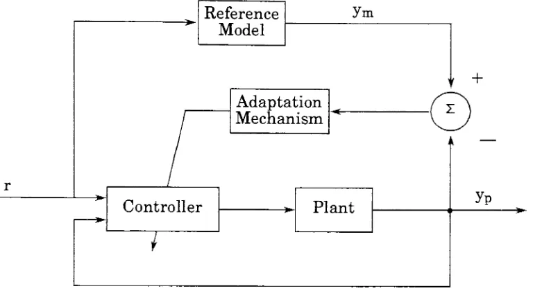
Two

principal approaches

to

adaptive control are

Model

Reference Adaptive

Control

(MRAC)

shown

in

Fig. #1

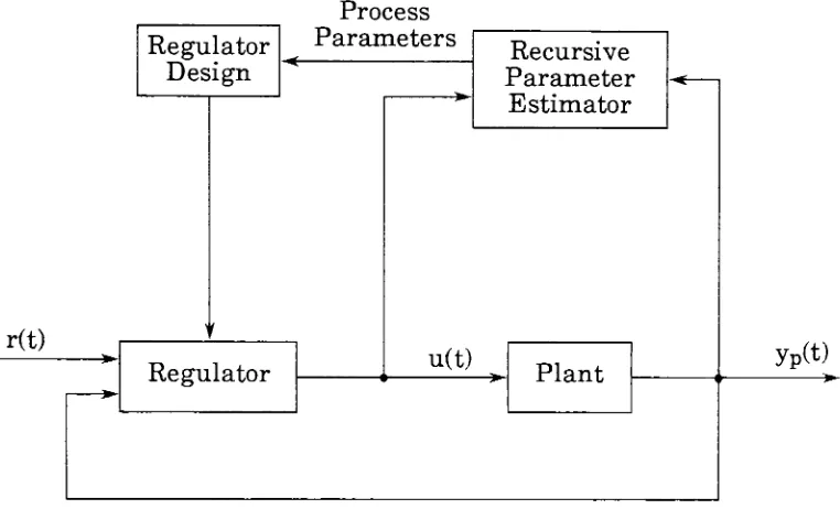
and

Self-Tuning

Regulator

(STR)

shown

in

Fig.

#2

[1].

The basic

principle of

MRAC

is

that the

performance of

the

system

is

specified

by

a model and

the

parameters of

the

regulatorare adjusted

based

on

the

error

between

the

reference model and

the

system.

MRAC

systems are

relatively easy to

implement

systemswitha

fairly

high

speed of

adaptation,

as

there

is

no need

for identification

the

plants parameters.

As

shown

in

Fig.

#1,

the

MRAC

system consistsof an

inner

loop,

whichprovides

ordinary

feedback

and an outer

loop,

whichadjusts

the

parametersof

the

inner

loop.

In

1973,

a major

breakthrough in

the

field

of adaptive control was

introduced

by

Astrom

and

Wittenmark,

the

idea

of a controller

that

could

tune

itself

and

actually

coined

the

phrase

'self

_{-tuning regulator'.}

The

original

self-tuning

regulator

(STR)

was

based

on stochastic minimum-variance principles and

least

squareestimation.

In

self-tuning,

the

basic

procedure

is

to

select a

design

Reference

Model

ym

Adaptation

Mechanism

Controller

Plant

t

+

0

A

yp

Figure

#1:

Model

reference adaptive control system

(MRAC).

recursively

estimatedvalues of

these

parameters.

The idea

of

using these

estimateseven

if

they

are notequal

to the true

values

(i.e.,

the

uncertainties are not_considered)

is

called

the

certainty

equivalenceprinciple.

STRs

are an

important

classofadaptive controllers.

They

are

easy to

implement

and are

applicable

to

complex

processes,

with a wide

variety

ofcharacteristics

involving

unknown

parameters,

the

presenceof

time-delay,

time varying

process

dynamics

andstochastic

disturbances.

The

closed

loop

systems [image:12.553.94.478.125.335.2]

r(t)

Regulator

Design

Process

Parameters

Regulator

Recursive

Parameter

Estimator

u(t)

Plant

[image:13.553.93.474.92.323.2]

yP(t)

Figure #2:

Self-tuning

regulator.

Two

approaches

to self-tuning

are

the

implicit

or

direct

STR

algorithm and

the

explicit or

indirect

STR

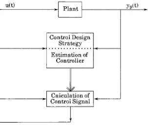
algorithm.

In

the

implicit STR

algorithm,

shown

in

Fig.

#3,

the

regulatorparameters are updated

directly.

Implicit

STRs

are

developed

on

the

basis

ofpredictivecontrol

theory

and require

knowledge

of

the

system

time

delay.

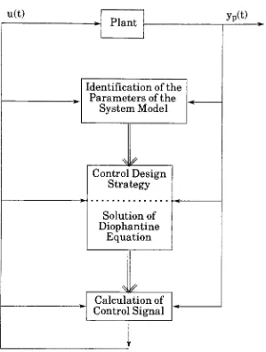
In

the

explicit

STR

algorithm,

shown

in Fig.

#4,

the

regulator parameter

identification

is followed

by

a separatecontrol

law

calculation.

The

system

time

delay

can

be

estimatedas part of

the

process

dynamics. Explicit STRs

u(t)

Plant

yP(t)

Control Design

Strategy

Estimation

of

Controller

^

Calculation

of

Control Signal

i '

Figure

#3:

Implicit

self-tuning

regulator. [image:14.553.161.464.102.358.2]

u(t)

Plant

yP(t)

Identification

of

the

Parameters

of

the

System Model

%.f

Control Design

Strategy

Solution

of

Diophantine

Equation

*

f

Calculation

of

Control Signal

[image:15.553.140.439.83.479.2]

''

Figure #4:

Explicit

self-tuning

regulator.

The

general

self-tuning

observer controller

(GSTOC),

shown

in

Fig.

#5,

is

a

form

ofexplicitself-

tuning

_{regulator which}

is

based

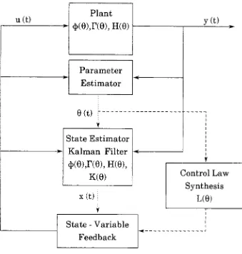
_{on modern control}

u(t)

Plant

4>(9),r(0),H(e)

Parameter

Estimator

9(t)

State Estimator

Kalman Filter

4>(9),r(0),

H(6),

K(0)

x(t)

State

-

Variable

Feedback

y(t)

Control Law

Synthesis

L(0)

Figure

#5:

General

self-tuning

observer controller.

polesare placed

based

on

the

modelparameters obtained

from

the

identification

scheme.

The basic

GSTOC

algorithm

is:

Identify

the

model parametersand

formulate

a state space model of

the

plant

{$(0),

T(0),

H(0)}.

[image:16.553.135.474.77.433.2]

Design

a control

law,

obtaining

L(0).

The GSTOC is

a

very

general algorithm as

it

does

not

specify

which methods

to

use

to

identify

the

plant model or choose

the

closed

loop

estimatororcontrol gains.

If

the

GSTOC

is

written

correctly

a subroutine call

to

the

different

parts

of

the algorithm,

different

estimation

techniques

such as

Recursive Least

Squares,

Recursive Maximum Likelihood

or

Stochastic

Approximation

Method

could

be

substituted

to

get

the

best

identification

method

for

the

job.

Same

reasoning

goes

for

the

estimator or control portions of

the

algorithm.

The

three

portions of

the

GSTOC

algorithmshown

in

Fig.

#5,

parameter

estimation,

state estimation and state variable

feedback,

are

developed in

the

3.

GSTOC

DESIGN

3.1

Parameter

Identification

Identification

is

the

experimental

determination

of

the

dynamic

behavior

of

processes and

their

signals.

[3]

For

adaptive control systems on-line

in

real

time

identification is

of

primary

interest

and an

important

part of

the

STR.

The

on-line methods give estimates

recursively

as measurements are obtained

and

is

the only

alternative

if

the

identification

is going

to

be

used

in

an

adaptive controller or

if

the

process

is

time-varying.[4] There

are

many

methods

for

analyzing

data

from

the

experiments.

Some

such methods are

Recursive

Least

Squares

(RLS),

Extended Recursive Least

Squares

(ERLS),

Recursive

Maximum Likelihood

(RML)

and

Stochastic

Approximation

Method

(STA).

The

recursive parameter

identification

technique

used

in the

GSTOC

developed in

this

paper will

be

Recursive Least

Squares. Given

the

linear

model

Z(k)

=

H(k)0(k)

+

V(k)

(3.1.1)

z(k)

z(k-l)

z(k-N-l)

and

z(k)

=

hT(k)0

+

_v(k).

The

_{estimation model}

for

Z(k)

is

Z(k)

=

H(k)0(k)

(3.1.2)

where

0 is

the

best

estimate of

0. The

principleof

least

squares states

that the

unknownparameters of

0

should

be

selected

in

such a

way that the

loss

function,

J(0(k))

=

Z(k)TZ(k)

(3.1.3)

is

minimal.

By

writing

(3.1.3)

as

J(0(k))

=

[Z(k)

-

Z(k)]'[Z(k)

-

Z(k)]

(3.1.4)

[Z(k)

-

H(k)9(k)]T[Z(k)

-H(k)0(k)]

(3.1.5)

=

ZT(k)Z(k)

-

2ZT(k)H(k)0(k)

+

0T(k)HT(k)H(k)0(k)

(3.1.6)

and

by

recalling that

d/dm(bTm)

=

b

and

d/dm(mTAm)

=

2Am

_{where m and}

b

dJ(9(k))/de(k)=

+

2HT(k)H(k)9(k)

(3.1.7)

by

setting

dJ(9(k))/d9(k)

=

0,

the

_{estimate of}

9 is

_given

by

9(k)=

[HT(k)H(k)l1HT(k)Z(k)

(3.1.8)

which

is

the

batch formula for

least

squares estimation.

To

develop

the

recursive

least

squares

equations,

in

(3.1.1)

&

(3.1.8)

it

was

assumed

that

Z(k)

contained

N

elements with

N

>

dim 9

= _n.

If

_another

sample

became

available at

t(k +

1),

it

would

be

very costly to

compute

9

using

(3.1.8). The

number of

flops

to

compute

9

is

on

the

orderofn3.

The

recursive

approach

is

to

compute

9 for

n =

ni

and

then

use

that

estimateof

9

to

obtain

9

for

n =

n2

where

n2

> ni.

One

additional measurement z(k

+

1)

at

t(k

+

1)

is

z(k

+

l)

=

hT(k

+

l)9(k)

+

_v(k

+

l)

(3.1.9)

Combining

the

additional measurementwith

(3.1.1)

and

from

(3.1.8)

9(k

+

l)

=

[H^k+DHCk + lttWk

+

lJZtk+l)

(3.1.10)

0(k

+

1)

=

[HT(k

+ l)H(k + DlHWk + l)z(k

+

1)

+

HT(k

+

l)Z(k

+

1)]

(3.1.11)

then

and

Z(k+1)

=

z(k

+

l)

Z(k)

H(k

+

1)

=

hT(k

+

l)

H(k)

V(k

+

1)

=

v(k

+

l)

* v-1*- -*/

V(k)

9(k)

=

P(k)HT(k)Z(k)

(3.1.12)

HT(k)Z(k)

=

P-!(k)9(k)

(3.1.13)

P-1(k

+

l)=P1(k)

+

h(k-r-l)hT(k

+

l)

(3.1.14)

9(k+l)

=

P(k

+

l)[h(k

+

l)z(k

+

l)+P1(k)9(k)]

(3.1.15)

:

P(k

+

l){h(k

+

l)z(k

+

1)

+

[Px(k

+

l)-h(k

+

l)hT(k

+

l)]9(k)}

(3.1.16)

=

9(k)

+

P(k

+

l)h[z(k

+

l)-hT(k+l)9(k)]

=

9(k)

+

K(k

+

l)[z(k

+

l)-hT(k

+

l)9(k)]

(3.1.18)

where

K(k

+

1)

=

P(k

+

l)h(k

+

l)

(3.1.19)

Equations

(3.1.14),(3.1.18)

and

(3.1.19)

are called

the

information

form

of

the

recursive

least

squares estimator.

9(0)

and

P_1(0)

can

be

initialized

to

0

and

I/a

(0<a<

<1)

respectively.

By

expressing

(3.1.18)

as

9(k

+

1)

=

[I-K(k

+

l)hT(k

+

l)]9(k)

+

K(k

+ l)z(k

+

1)

(3.

1

.20)

it

can

be

seen

that

the

recursive

least

squaresestimator

is

a

time-varying

digital filter

that

is

excited

by

random

inputs. There is

acomputationcost

in

inverting

the

n xnmatrix

P

of

(3.1.14).

By

applying the

matrix

inversion

lemma

which

is

B1 = A1

+

CTJ^C

(where

all matrix

inversions

are assumed

to

exist,

A

and

B

are nx

n,

C

is

mxn

and

D is

m xm)

then

to

(3.1.14)

results

in

P(k

+

1)

=

P(k)-P(k)h(k+l)[hT(k-r-l)P(k)h(k

+

l)+I]1hT(k

+

l)P(k)

(3.1.21)

and

consequently,

by

substituting

(3.1.12)

into

(3.1.19)

for P(k

+

1)

and

simplifying

K(k

+

1)

=P(k)h(k+l)[hT(k

+

l)P(k)h(k

+

l)

+I]"1

(3.1.22)

and

simplifying

(3.1.21)

P(k

+

l)

=

P(k)

K(k

+

l)hT(k

+

l)P(k)

(3.1.23)

P(k+1)

=

[I-K(k

+

l)hT(k

+

l)]P(k)

(3.1.24)

Equations (3.

1.18),

(3.

1.22)

and

(3.1.24)

are

the

covariance

form

of

the

recursive

least

squares estimator.

9(0)

and

P(0)

can

be initialized

to

the

same values as

in

the informational

form.

It

can

be

seen

that

if

z(k)

is

scaler, then

the

covariance

form

of

RLS

requires no matrix

inversion,

and

only

one

division.

In

the

development

of

the

RLS

formulas

all

the

measurements were weighted

by

the

same amount.

In

the

caseof

time-varying

parameters,

a

forgetting

or

than

pastones.

By

introducing

a

weighting

matrix

W

which

is

diagonal

into

(3.1.3)

J(9(k))

=

Z(k)TWZ(k)

(3.1.25)

Then

(3.1.8),

(3.1.14)

and

(3.1.19)

could

be

written as

9(k)

=

[HT(k)WH(k)]1HT(k)WZ(k)

(3.1.26)

P1(k

+

l)

=

P1(k)

+

h(k

+

l)w(k

+

l)hT(k

+

l)

(3.1.27)

K(k

+

1)

=

P(k

+

l)h(k

+

l)w(k

+

l)

(3.1.28)

and

(3.1.22)

as

K(k

+

1)

=

P(k)h(k

+

l)[hT(k

+

l)P(k)h(k

+

l)

+w(k +

l)f1

(3.1.29)

the

weighted recursive

least

squareestimator

(covariance

form)

equationsare

9(k

+

l)

=

9(k)

+

K(k

+

l)[z(k

+

l)-h(k

+

l)9(k)]

(3.1.30)

K(k

+

1)

=

P(k)hT(k + l)[h(k

+

l)P(k)hT(k

+

l)

+

w(k-r-l)]-1

(3.1.31)

P(k)

=

[I

-

K(k)h(k)]P(k-l)/w(k

+

3.2

Discrete

Kalman

Filter

(Optimum

Observer)

A

dynamic

system whose statevariablesare

the

estimates of

the

state variable

ofanothersystem

is

called anobserver of

the

latter

system.

The

state

estimator

that

is

optimum with respect

to the

process noise and observation

noise

is

called a

Kalman

filter.

The Kalman

filter

_was

first introduced

by

R. E.

Kalman

in 1960

for discrete

systems.

In

the

development

of

the

GSTOC

a

recursive

discrete Kalman filter

with

time varying

gainswill

be implemented.

The

plant will now

include

processandmeasurementnoise.

x(k

+

l)

=

<Sx(k)

-r-Tu(k)

+

w(k)

(3.2.1)

z(k) =

Hx(k)

+

v(k)

(3.2.2)

where

w(k)

andv(k) are

the

process andmeasurementnoise and are assumed

to

be

uncorrelatedand

have

gaussian

distributions.

Where

E{w(i)wT(j)}

=

Q(i)8

(3.2.3)

E{v(i)vT(j)}

=

R(i)8..

(3.2.4)

E{w(i)vT(j)}

=

S

=

₀

(for

_all

i

_and

j)

(3.2.5)

and

the

covariance matrix

Q(i)

is

positive semidefinite and

R(i)

is

positive

definite

so

that the

inverse

R_1(i)

exists.

Disturbance

w(k)

may

be

disturbance forces

acting

on

the

system,

errors

in

modeling,

system errors

due

to

actuators or errors

in

the

translation

of

the

known

input

u(k)

into

physicalsignals.

The

disturbance

v(k)

is

often used

to

model errors

in

the

measurements made

by

the sensing

instruments,

unavoidable

disturbances

that

act

directly

on

the

sensors and errors

in

the

state

x(0)

is

unknown

but

the

mean

E{x(0)}

=

mx(0)

_{and covariance}

Px(0)

_are

known

and

x(0)

is

uncorrelated with_w(i)and v(i).

To derive

the

recursive

equations

for

the

discrete Kalman

filter,

the

propagation of

the

means and

covariancesof

the

system

(3.2.1)

and

the

effects of

the

measurements

(3.2.2)

need

to

be investigated.

Taking

the

expected value of

(3.2.1)

E{x(k

+

1)}

=

E{Ox(k)

+

Tu(k)

+

^Fw(k)}

(3.2.6)

and

using

the

linearity

of

the

expectation operator results

in

E{x(k+

1)}

=

E{$x(k)}

+

E{Tu(k)}

+

E

pFw(k)}

(3.2.7)

and

E{x(k

+

1)}

=

$E{x(k)}

+

TE{u(k)}

+WE

{w(k)}

(3.2.8)

because

of

<I>,

W,

T

are

deterministic.

Also

because

_u(k)

is

a

known input

and

E{w(k)}

=

₀

from

being

gaussian,

equation

(3.2.8)

can

be

reduced

to

E{x(k

+

l)}

=

<DE{x(k)}+ru(k)

(3.2.9)

The

state covariance

Px(k),

which

is defined

as

E{(x(k)

-mx(k))(x(k)

-mx(k))T}

propagates as:

Px(k

+

1)

=

E{[x(k

+

l)-mx(k

+ l)][x(k+l)-mx(k

+

l)]T}

(3.2.10)

= <DPx(k)0T

+

^Q(k)T

+

OE{[x(k)

-mx(k)]wT(k)WT}

+

WE{w(k)[x(k)

- mx(k)]T}<DT

(3.2.12)

Because

mx(k)

is

notrandom andw(k)

is

zero

mean,

E{mx(k)wT(k)}

=

mx(k)

_and

E{wT(k)}

=

0 along

with

E{w(k)mxT(k)}

=

0.

Since

the

_{state vector}

x(k)

depends

at

the most,

on random

input

w(k-l)

then

E{x(k)wT(k)}

=

E{x(k)}E{wT(k)}

=

₀

and

E{w(k)xT(k)}

=

0 then

(3.2.12)

_reduces

down

to

Px(k

+

1)

= $Px(k)$T

+

iJ/Q(OTT

(3.2.13)

The first

term

of

(3.2.13)

is

due

to the uncertainty

in

the

plant and

the

second

term

is

due

to

the

process noise w(n).

To determine

the

means and covariance of

the

output

take

the

expected value

of(3.2.2)

mz(k) =

E{z(k)}

=

HE{x(k)}

=

Hmx(k)

(3.2.14)

with

Ev(k)

=

₀

from

being

gaussian.

The

cross covariance

between

the

state and

the

output

is

Pxz(k)

=

E{[x(k)

- _mx(k)][z(k)

-mztk)]7}

(3.2.15)

=

E{[x(k)

- _{mx(k)][H(x(k)}

-mx(k)

+

v(k)]T}

(3.2.16)

=Px(k)HT

(3.2.17)

Pz(k)

=

E{[z(k)

-mz(k)][z(k)

-mz(k)]T}

(3.2.18)

=

E{[H(x(k)

-mx(k)

+

v(k)][H(x(k)

-mx(k) +

v(k)]1)

(3.2.19)

= HPx(k)HT

+

R

(3.2.20)

Defining

the

a priori estimationerrorcovariance at

time

k

as

x(k|k-l) = _x(k)

-x(k|k-l)

(3.2.21)

and

the

associated a priori error covariance as

P(k|k-1).

The

estimateat

time

k

including

the

output measurement

z(k),

be denoted

by

x(k|k).

The

aposteriori

estimationerror

is

then

x(k|k) = _x(k)

-x(k|k)

(3.2.22)

and

the

associated aposteriori error covariance as

P(k|k).

The

Kalman

filter has

two

steps ateach

time

k. The

time

update which

is

x(k-l|k-l)

updated

to

x(k|k-l)and

the

measurementupdate

in

which

the

measurementz(k)updatesx(k).

The

time

updatesof

(3.2.9) & (3.2.13)

are

x(k|k-l) =

<Dx(k-l|k-l) +

Tu(k-l)

(3.2.23)

P(k|k-1)

= <DP(k-l|k-l)^T

+

*FQ(k-OTT

(3.2.24)

The

measurementupdateof

the

Kalman filter

will

involve

computing the

x(k|k)

=

Fz(k)

+

g

(3.2.25)

The

matrix

F

and

the

vector

g

need

to

be determined

for

the

optimal

linear

estimate of

x(k)

givenz(k).

By

minimizing

the

mean-squarederror of

J

=

E{x(k|k)xT(k|k)}

(3.2.26)

=

E{tr[(x(k)

-x(k|k))T(x(k)

-x(k|k))]}

(3.2.27)

=

E{tr[(x(k)

-x(k|k))(x(k)

-x(k|k))T]}

(3.2.28)

=

E{tr[(x(k)

-Fz(k)

-g)(x(k)

-

Fz(k)

-g)T]}

(3.2.29)

=

E{tr[(x(k)-x(k|k-l)-(Fz(k)

+g-x(k|k-D)

(x(k)

-x(k|k-l)

-(Fz(k)

+

g

-x(k|k-l))T]}

(3.2.30)

by

substituting

mz(k) =

Hx(k|k-1)

_and

Pzx(k)

=

E{(z(k)

-mz(k))(z(k)

-mz(k))T}

into

(3.2.30)

J

=

tr[P(k|k-l)

+

F(Pz(k)

+

mz(k)mzT(k))FT

+

(g

-

x(k|k-l))(g-x(k|k-l))T

+

2Fmz(k)(g-x(k|k-l))T

-2FPzx(k)]

(3.2.31)

by

using

d/dF tr(FXTT)

=

2FX

and

d/dF

tr(DFX)

=DTXT

(for any

matrix

F,D

and

X).

J

=

2F(Pz(k)

+

_{mz(k)mzT(k))-2Pzx(k)}

+

2(g-x(k|k-l)mzT(k))

+

(g-x(k|k-l))(g-x(k|k-l))T

Thus

to

minimize

J it

is

required

that

5J/8g

=

2(g

-x(k|k-l)) +

2Fmz(k)

=

₀

(3.2.33)

and

8J/8F

=

2F(Pz(k)

+ mz(k)mzT(k))

-2Pxz(k)

+

2(g

-x(k|k-l)mzT(k))

=

0

(3.2.34)

solving

for

g

from

(3.2.33)

g

=

x(k|k-l)-FmzT(k)

(3.2.35)

substituting

g

from

(3.2.35)

into

(3.3.34)

results

in

FPz(k)

Pxz(k)

=

₀

(3.2.36)

and

solving

for F

F

=

Pxz(k)Pz-1(k)

(3.2.37)

substituting

(3.2.35)

&

(3.2.37)

into

(3.2.25)

gives

the

optimal

linear

mean-squared estimate

for

_x(k)

x(k)

=

x(k|k-l) +

Pxz(k)Pz-1(k)(z(k)

-mz(k))

(3.2.38)

replacing

Pxz(k),

Pz_1(k)

and

mz(k)

with

previously

computed values

from

(3.2.17),

(3.2.20)

and

(3.2.14)

and

the

appropriate substitutions

for

P(k|k-1)

and

x(k|k-l)

into

(3.2.38)

result

in

x(k|k) = _x(k|k-l)

+

P(k|k-l)HT(HP(k|k-l)HT

+

R)1(z(k)

Equation

(3.2.39)

is

the

optimal

linear

estimate a posteriori estimate ofx(k)

given

the

a priori estimate

x(k|k-l)

and

the

new measurement z(k).

In

computing the

a posteriori error covariance

P(k|k)

it is known

that the

linear

mean-squared estimate

is

unbiased

E{x(k)}

=_mx(k)or

E{x(k|k)}

=

₀

_and

using

(3.2.38)

E{x(k|k)}

=

E{x(k)

-x(k|k)}

(3.2.40)

-

E{(x(k)

-x(k|k-l))

-Pxz(k)Pz"1(k)(z(k)

-mz(k))}

(3.2.41)

=

E{x(k)

-x(k|k-l)}

(3.2.42)

=

E{x(k|k-1)}

(3.2.43)

Therefore,

x(k|k)provides anunbiasedestimateofx(k)as

long

asx(k|k-l)

is

unbiasedand

from

(3.2.1)

and

(3.2.9)

E{x(k|k-1)}

=

E{x(k)

-x(k|k-l)}

(3.2.44)

=

E{x(k)

-Ox(k|k)

-Tu(k-l)

(3.2.45)

=

$E{x(k-l)

-x(k|k)}

(3.2.46)

=

0>E{x(k|k)}

(3.2.47)

shows

that

x(k|k-l)providesanunbiased estimate

if

x(k-l|k-l)

does. If

the

x(0) =

mx(0)

(3.2.48)

which

is

known,

then the

initial

estimate

is

unbiased.

Using

(3.2.38)

to

find

P(k|k)

P(k|k)

=

E{x(k|k)xT(k|k)}

=

E{(x(k)

-x(k|k))(x(k)

xfklk))1}

(3.2.49)

=

E{[(x(k)

-x(k|k-l))-

Pxz(k)Pz1(k)(z(k)

-mz(k))]

[(x(k)

-x(k|k-l))

-Pxz(k)Pz1(k)(z(k)

-mz(k))]T}

(3.2.50)

=

P(k|k-1)

-Pxz(k)Pz1(k)Pzx(k)

-Pxz(k)Pz'1(k)Pzx(k)

+

Pxz(k)Pz1(k)Pz(k)Pz"1(k)Pzx(k)

(3.2.51)

or

P(k|k)=

P(k|k-1)

-

PxzCWPz-HkJP^k)

(3.2.52)

Using

(3.2.17)

& (3.2.20) into

(3.2.52)

with

the

appropriatesubstitution

by

P(k|k-1)

P(k|k)

=

P(k|k-1)

+

R^HPtelk-l)

(3.2.53)

Equation

(3.2.53) is

known

as

the

matrix

Riccati

equation

for

P(k|k)

or

by

using the

matrix

inversion

lemma

P(k|k)= [P(k|k-l)-1

+

(HTR-1H)-1l-1

(3.2.54)

K(k)

= P(k|k-l)HT[HP(k|k-l)HT

+

RJ-^PCklkJlTR-1

(3.2.55)

then

(3.2.39)

could

be

written as

x(k|k)

=

x(k|k-l) +

P(k|k)HTR"1[z(k)

-

Hx(k|k-1)]

(3.2.56)

x(k|k) =

x(k|k-l) +

K(k)[z(k)

-Hx(k|k-1)]

(3.2.57)

K(k)

is

the

Kalman

gain matrix and

it

show

the

influence

of

the

new

measurement

z(k)

in

modifying the

aprioriestimate x(k|k-l).

The

quantity

[z(k)

Hx(k|k-1)]

is

called

the

residual and

is

an apriorioutputestimation

error,

since

Hx(k|k-1)

providesanestimate of

the

output.

Substituting

K(k)

into

(3.2.53)

gives

P(k|k)=

[I-K(k)H]P(k|k-l)

(3.2.58)

The

recursive equations

for

the Kalman filter

are:

x(k|k-l) =

<x(k-l|k-l)

+

Tu(k-l)

(3.2.23)

x(k|k) = _x(k|k-l)

+

K(k)[z(k)

-

Hx(k|k-1)]

(3.2.57)

K(k)

= P(k|k-l)HT[HP(k|k-l)HT

+

R]"1

(3.2.55)

P(k-l|k-l)

=

[I

3.3

Control Law

In

control system

design

it is

desirable

to specify the

closed-loop

dynamic

performanceof

the

system under control or

optimally

control

the

state

variables and or

the

control variable.

The design

of

the

controller results

in

the

assignment of

the

poles of

the closed-loop transfer

function,

the

method

is

known

as pole-placement.

Pole-placement

using

state variable

feedback

is

whereall

the

internal

states are available

for feedback

either

in their

measured

quantity

or

their

estimated quantities.

Pole-placement

design

can

speed

up the

response of a sluggish system.

The

procedure

in

finding

the

gain

matrix

L

ofthe

GSTOC

willuse

Ackerman's

formula. Ackerman's

formula

is

based

on a

transformation

from

ageneral system matrix

$

to that

of a control

canonical

form. Given

the

discrete

single-input single-output state space

model

x(k

+

l)

=

<J>x(k)

+

Tu(k)

(3.3.1)

and

choosing the

control

input

u(k)

to

be

a

linear

combination of

the

states

u(k) = _-Lx(k)

(3.3.2)

where

L

=

[h 12 13

-..

InJ

(3-3.3)

x(k

+

l)

=

(4>-rL)x(k)

(3.3.4)

Given

the

characteristicequation

P(z)

= zn

+

Pn-iz""1

+

pn-2Zn"2

+

....

+P1Z+ pn

(3.3.5)

If

the

system of

(3.3.1)

is in

the

control canonical

form

shown

in

(3.3.6)

x(k

+

l)

=

0

10

0

0

1

0

0

-an -ai -Q2 -an-i

x(k)

+

0

0

u(k)

(3.3.6)

with

the

characteristic equation

a(z) = |zl-

A|

= zn -l-an.iz11-1

+

an.2zn-2

+

+

aiz

+a0

(3.3.7)

TL

=

0

0

h

h

l3

....

In

0

0

0

....

0

0

0

0

....

0

h

I2

13

....

In

(3.3.8)

Then

the

closed

loop

system matrix

is

0

0

1

0

0

1

0

0

-(an

+

li)

-(ai+l2) -(02

+ 13)

....

-(an-i

+

ln)

(3.3.9)

and

the

characteristic equation of

|zl-d>

+

TL|

as

zn +

(Qn-i

+

ljz11-1

+

(an-2

+

ln-l>n-2

+

...

+

(ai

+

l2)z+

(an

+

U)

(3.3.10)

then

by

equating

coefficients

in

(3.3.5)

&

(3.3.10)

results

in

the

gains

li+1

=

In

general

the

system under

interest is

not

in

control canonical

form. Given

that the

system

is

reachable,

a

transformation

matrix

T

needs

to

found

to

convert

the

system

to the

form

of

(3.3.6).

By

defining

an

arbitrary

transformation

of

the

state vector

x(k)

to

w(k)

by

Tx(k)

=

w(k)

(3.3.12)

the

new set of state equations are

x(k

+

1)

=

<>x(k)

+

Tu(k)

(3.3.13)

w(k+

1)

=

T$x(k)

+

Tu(k)

(3.3.14)

w(k

+

l)

=

TtfPMk)

+

TTu(k)

(3.3.15)

For

the

correct choiceof

T,

T<J>T_1can

be

put

into

control canonical

form. Define

Tr^T"1

as

4>c

and

TT

as

Tc.

By defining

a matrix called

the controllability

matrix

wc

=

cr

$r

...

$n2r

4>nlr]

(3.3.16)

and

wcc

=

[rc

<j>crc

...

(>cn-2rc

<$>cnlrc]

(3.3.17)

Wcc

=

[TT

(Tr^T-^TT

...

(TtfT^Tr

(T$T1)n-1Tr]

(3.3.18)

T

= WCCWC1

(3.3.20)

P($)

=

$?+

pi^11"1

+

p2$n-2

+

+pnI

(3.3.21)

where<J)

is

the

system matrixof

the transformed

system

(3.3.6). Then

by

using

the

Caley-Hamilton

theorem

P($)

= in

+

(pi-ai)^-1

+

(p2-a2)rin-2

+

+(Pn-an)I

(3.3.22)

The

last

row of<k

is

zero except

in

position n-k which

is

then

t

=

[0

0

0

0

1]P($)

(3.3.23)

but

^=(T$T-X)

then

L

=

Z.T

=

[

00

0

0

UPOtyT-^T

(3.3.24)

=

[0

0

0

0

1]TP($)

(3.3.25)

butT

=

WccWc-1and[0

0

0

0

1]WCC

=

[

0

0

0

0

1],

then

L

=

LWCC

Wc"1 =

[

0

0

0

0

UW^P^)

(3.3.26)

which

is

Ackerman's formula.

Given

the

desired

matrixpolynomialac(

A)

=

An

+

an-iAnl

+

...

4-anl.

Then

l

=

to o o

...

i] [

r

<j>r...<r2r

^ri-1

The

next question

that

needs

to

be

answered

is

where should

the

closed

-loop

poles

be

placed.

Some

guideline

that

govern

the

choice of

the closed-loop

poles

are:[5]

Select

a

bandwidth high

enough

to

achieve

the

desired

speed of response.

In

practical

systems, there

are

limits

on

the

control

input. If

the

controlsignal

generated

by

the

linear feedback law

u(k) = _-Lx(k)

is

larger

than

possible

or

permissible, there may

be

potential

damaging

effects

to the

plantor

drive

the

plant

into

a non-linear region and

(3.3.1)

will not

accurately

model

the

plant.

Keep

the

bandwidth low

enough

to

avoid

exciting

unmodeled

high-frequency

effects andundesired response

to

noise.

Place

the

poles at

approximately

uniform

distances

from

the

origin

for

efficient useof

the

controleffort.

The broad

guidelines above allow

plenty

of

latitude for

the

specialneedsof

individual

applications.

As

aresult

from

optimization

theory,

closed

loop

poles

in the

"Butterworth"

configuration

is

often suitable placement.

The

"Butterworth"

configuration

places

the

poles

radially

at anuniform

distance from

the

origin

in left half

plane.

The

roots of

the Butterworth

polynomialsare given

by:

(s/o0)2m ₌ (-Dm+1

(3-3-28

)

The

farther

away

from

the

open

loop

poles,

the

closed

loop

poles are

placed,

the

gains

to

effect a change

in

the

system poles.

Bandwidth

is

determined

primarily

by

its

dominant

poles,

i.e.,

the

poles with real parts closest

to the

4.

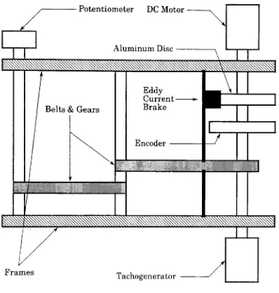
PLANT DESCRIPTION

4.1

Plant

A LJE DC

motor

module,

a general

diagram

shown

in Fig.

#6,

will

be

used as

the

plant

in

order

to

develop

the

GSTOC. The DC

motor

is

a

Phillips

model

MB-12. The

motor

is

capable of

being

driven

at speeds of

up to

2,500

rpm

in

either

direction.

An

analog

voltage

in

the

range of+/-

5

volts

determines

the

speed and

direction

of rotation.

A

second

DC

motor

driven

directly by

the

first

provides an

analog

feedback

voltage

in

the

range of +/-

5

voltsproportional

to

the

speed and

direction

of rotation.

An

eddy

current

brake,

which uses a

permanent magnet

to

create a magnetic

field

in

which analuminum

disc

rotates,

is

used

to

introduce torque

disturbances

on

the

motor.

The

brake has

three

settings:

1.

OFF,

2.

Mid

position, 3.

Fully

On. The

motor module also

has

a continuous rotation

potentiometer,

which

is driven

by

an output shaftgeared

down

by

a ratio of

9:1

from

the

motor.

The

potentiometergives an

analog

feedback

voltage

in

the

rangeof +/-

2.5

voltsproportional

to the

position of

the

Potentiometer

DC Motor

Belts & Gears

Eddy

Current

-Brake

Encoder

misn

J

HUHMliMiaWi yuSiittmSStMiii^k

Frames

[image:43.553.79.477.86.504.2]

Tachogenerator

4.2

MATHEMATICAL

MODEL

The

mathematicalmodel of a

the

LJE DC

servo motor used

in

this

application

will

be developed

in

this

section.

The

generalelectrical characteristics of a

DC

motor

is:

L

di(t)/dt

+

R

i(t)

=

V

-emf

(4.2.1)

where

L

is

the

inductance

of

the

motor armature

(henries)

R

is

the

resistance of

the

motor armature

(ohms)

V

is

the

applied voltage

(volts)

i(t)

is

the

current

through the

armature

(amps)

di(t)/dt

is

the

instantaneous

current

(amps/sec)

emf

is

the

back

emf=

Ke

d9(t)/dt

where

Ke

is

a constant

(Volts/rad/sec)

d9(t)/dt is

rotational

velocity

(rad/sec)

The

general mechanicalcharacteristics of a

DC

motor

is:

Jm

d29(t)/dt2

+

Bd9(t)/dt

+

K9(t)

=

TL

- JLd29(t)/dt2

(4.2.2)

where

Jm

is

the

motor

inertia

(Kg

m2)

9(t)

is

rotational position

(rad)

d9(t)/dt is

rotational

velocity

(rad/sec)

d29(t)/dt2

K

is

a stiffness constant

(N

m/rad)

B

is

a

damping

constant

(N

m/rad/sec)

JL

is

the

load inertia

(Kg-m2)

TL

is

the

load

torque

=

Kp

i(t)

where

KT

is

the torque

constant

(N-m/A)

i(t)

is

the

current

through the

armature

Combining

and

simplifying

4.2.1

&

4.2.2

and

assuming that the

electrical

time

constant

is

much shorter

than the

mechanical

time

constantyields

d29(t)/dt2 ₌

Kj/JR

*

V

-

(B/J

+

KT

Ke/JR)

*

d9(t)/dt

(4.2.3)

Letting

x(t) = d29(t)/dt2

x(t) =

d9(t)/dt

the

scaler modelof

the

DC

motorcan

be

defined

as

x(t) =

KT/JR

*_u(t) -

(B/J

+

Kp

Ke/JR)

* x(t)

(4.2.4)

Substituting

the

LJE DC

motorparameter values

R

=

2

ohms

Kt

=

0.007 N-m/A

Ke

=

0.008 V/rad/sec

B

=

30.3 E

10'6

N-m/rad/sec

Jm

=

17.5

E

10"6Kg-m2

the resulting

equation of

the

unloaded

DC

motor

is:

x(t) =

3.4

u(t)

-

3.331

x(t)

(4.2.5)

Using

the

Matlab function

c2d and a

sampling time

of

lOmSec

the

discrete

scaler model of

the

DC

motor

is:

x(k

+

1)

=

0.96723867

x(k)

+

0.03344

u(k)

(4.2.6)

wherex(k)

is

rotational

velocity

state and_u(k)

is

the

control voltage.

Equation

(4.2.6)

is

of

the

form (3.3.1).

The loaded

scaler model of

the

DC

motor was

found

experimentally

and

the

resulting

equation

is:

x(t) =

5.59

_u(t) -

5.4795

x(t)

(4.2.7)

and

the

discrete

equation

is:

5.

DSP

IMPLEMENTATION

5.1

Parameter Identification

In

the

parameter

identification

part of

the

GSTOC,

which uses

the

RLS

informational

form

with a

forgetting

factor,

the

unknown parameters of

9 in

(3.1.1)

that

were

estimated,

are

$

and

T

of

(3.3.1). The

values of

H

of

(3.1.1)

are

known functions based

on

the

pair of observations

z(k)

and

u(k)

obtained

in

the

experiment.

The

recursive equations

(3.1.30),

(3.1.31)

and

(3.1.32)

were used

in

the

GSTOC

algorithm.

Bierman's

U-D

covariance

factorization

method

[7]

wasused

in

the

RLS

estimation

for

the

matrix

P(k)

in (3.1.32).

The

factorization

offers computational

savings,

numerical

stability

and reductions

in

computer storage requirements.

The

factorization

states

that

matrix

P(k)

can

be

factored

as

P

=

U D

UT

with

U

as an unit upper

triangular

matrixand

D

is

a

diagonal

matrix.

Computing

with

triangular

matrices

involves

fewer

arithmetic

operations,

which

is

preferred

in

a real

time

applications.

A

three

variable

forgetting

factor

was also used

in the

algorithm.

The

three

values were:

none,

if

the

estimation errorwas

less

than

acertain

value,

no update was

done,

a value of

0.999

for

slowly changing

parametersand a value

of

0.95 for

fast

changing

parameters.

The

initial

values

for 9 in

(3.3.1)

were

the

loaded

experimentally

obtainedvalues of

$

and

V

of

(4.2.8).

5.2

Kalman Filter

The

Kalman

filter

will

be

implemented

withstraight

line

coding

of

the

computations.

The

value

for

R in

(3.2.55)

was

determined from data

obtained

from

the

experiments.

The

value

for

Q

in

(3.2.24)

was chosen

to

give

the

best

results.

The initial

values

for

P(k-l|k-l)

in

(3.2.58),

P(k|k-1)

in

(3.2.4)

and

K(k)

in

(3.2.55)

wereobtained

using

the

DLQE

Matlab function

on

the

parameters

from

(4.2.8)

and

the

chosenvaluesof

R

and

Q.

5.3

Control Law

The

computing

of

the

gain matrix was

implemented

with straight

line

coding

of

Ackerman's formula (3.3.27).

The initial

value of

the

pole

for

the

desired

characteristicequation was chosen as not

to

produce a

large

valued gain

matrix.

5.4

Scaling

When

using

fixed-point

arithmetic

it

is

usually necessary to

perform

scaling

on

the

controller

to

be

implemented.[6]

Two

objectivesof

scaling

are

to

fit

the

data

which

is

computed

during

the

course of stateequationcalculations

into

the

limited

number range of

the

DSP,

so

that

overflows are avoided without

provoking

excessive signal quantation effects and

the

other

is

to

alter

the

coefficients

in

such a

way that

they

fit

into

the

coefficientnumberrange.

Input /

output

scaling transforms the internal

fractional

representations ofa

number

to

the

external physicalvariables.

The

input

to the

motor

(output

of

the

D/A)

is

+/-

5

_volts.

A

-I-1 to

-1

in

the DSP

would represent a

+

5

volt

to

-5

volts

input

to the

motor.

The

scaling

of

the

numbers used

the

GSTOC

algorithm

had

to

be

watch

carefully

so as not

to

overflow

the

computed

5.5

Division

Since

the

TMS320C25 doesn't have

a

divide

instruction,

a

way

of

doing

an

inverse

operation

had

to

be implemented.

One

way to

accomplish

this

is

to

use

approximation

techniques

using

the

solution ofnon-linearequations.

This

methodrequires

that

a solution

for

the

equation

g(x)

=

₀

(5.5.1)

be

found. One

means

for

find

a solution

for

(5.5.1)

is

by

Newton-Raphson

iteration.

Consider

the

Taylor

series expansion

for

g(x):

g(x

+

h)

=

g(x) +

hg\x)

+

_r(x,h)

(5.5.2)

wherer(x,h)

is

the

remainder andcan

be

consideredsmall andg'(x)

is

the

first

derivative

of g(x).

Leaving

off

the

remainderand

in terms

of

incremental

valuesofx

the

approximation:

g(x[i

+

l])

= _g(x[i])

+

{x[i

+

l]

_{x[i]}g'(x[i])}

(5.5.3)

Solving

for

x[i

+

1]

and with

g(x)

=

₀

_yields

the

_{approximation}

x[i

+

1]

= _x[i]

-g(x[i])/g'(x[i])

(5.5.4)

thus

x[i

+

1]

willconverge

to

asolution ofg(x) =

0.

To

find

an

inverse

ofanumberc

(1/c)

onecanwrite:

g(x[i]) =

l/x[i]

-c =

0,

(5.5.5)

substituting

in

(5.5.4)

and

simplifying

gives:

x[i

+

l]

=

x[i]{2-cx[i]}

(5.5.6)

The

initial

guess

for

x[0]

canalso

be

approximated.

The

inverse

ofcas:

1/c

= l/m*2-e

(5.5.7)

A

good seed

for

the

iteration

of

the

inverse

of c would

be

2e.

One

must

take

precautions

using this

method

in

that

for

certainvaluesof

c,

6.

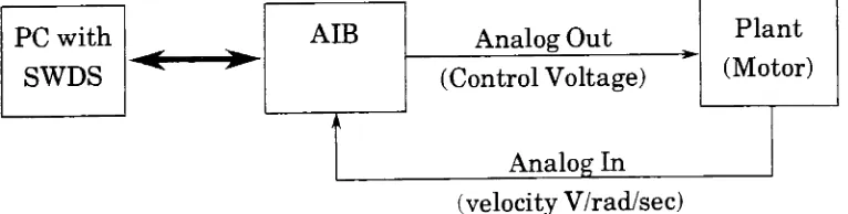
HARDWARE DESCRIPTION

A

TMS320

Analog

Interface Board

(AIB)

provided an

interface

from

the

TMS320C25

to the

plant.

The AIB

is

an

analog-to-digital,

digital-to-analog

conversion

board

used as a

preliminary

target

system with

the

SWDS

or

in

a

standalone configuration.

The

AIB

has

the

following

setof

features:

A

16

-

bit

Analog

to

Digital

Convertor

with a-10V

to

+

10V analog

input

range with a maximum conversion

time

of

17uSec.

A 16

-

bit Digital

to

Analog

convertor witha-10V

to

+

10V

analog

output

range with a

3uSec

settling time.

Sampling

rateclock withaprogrammablerange of

5MHz to 76Hz

witha

usable range of

58.8KHz to 76Hz

(limited

by

the

conversionrangeof

the

A/D).

On-board

memory 4K

x

16

to 64K

x

16 for

standaloneoperation. [image:51.553.95.478.454.551.2]

Anti-aliasing

and

smoothing

filters.

Fig. #7

showsa

block diagram

of

the

system configuration used

in the

GSTOC,

PC

with

SWDS

AIB

Analog

Out

Plant

(Control

Voltage)

Analog

In

(Motor)

,*

(velocity

V/rad/sec)

7.

DSP CODE

The

development

and

testing

of

the

GSTOC

algorithm was

done

on

the

Texas

Instruments Software Development System (SWDS). The SWDS

is

a

PC-resident software

development/debugging

tool

with

the

following

features:

Full

speed

40

MHz TMS320C25 DSP

48

Kbytes (24 K

16-bit

words) of no wait state

RAM

RAM

configurable

between

program and

data

space

memory

8

breakpoints

on

instruction

acquisition

Window-oriented

debugger

screen

Data

logging

allowing

I/O

operations

to

disk

files

The

complete

GSTOC

code

is

listed in Appendix A. The

code

for

the

GSTOC

algorithm

is

organized as

follows:

INITIALIZE

load

constants

from

program

memory to

data

memory

clearvariables

initialize

AIB

board

wait

for

interrupt

ISRO

get

input

z(k)

compute

ERR

= _z(k) - _ye(k|k-l)

Parameter Estimation

computepredictionerr

PERR

=

HT(k)

*

THETA(k)

update

diagonal,

off-diagonalelementsof

P

and

the

gain values

U(i,i),U(ij)

andB

B*PERR

State Estimation

update

the

covariancematrix

calculate

the

Kalman

gainvalues

update

the

state estimate

update

the

errorcovariancematrix

Pole-placement

Gain

calculate

the

gain matrix

GSTOC

calculate

x(k|k)

calculate

the

control signal

v(k)

saturate

the

control signal

u(k)

update

the

estimate_x(k|k-l)

return

to

wait

for interrupt

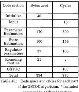
By

using the timer

on

the

TMS320C25,

the

number of cycles

for

eachpart of

the

GSTOC

algorithm was

determined,

and

the

results are shown

in

Table #1.

From Table

#1 the

total

execution

time

for

the

interrupt

service routine

is

77uSec,

therefore the

maximum

sampling

frequency

is 12.9 KHz. This

Code

section

Bytes

used

Cycles

Initialize

40

Input

15

Parameter

Estimation

170

390

State

Estimation

100

156

Regulator

parameters

37

106

Rounding

routine

21

*

GSTOC

103

[image:54.553.148.406.74.373.2]

Total

394

770

Table #1:

Code

space and cycles

for

eachpart

of

the

GSTOC

algorithm. *

included

8.

RESULTS

The data for

the

following

graphswere obtained

by

sampling

the

output

using

the

analog to

digital

converteron

the

AIB. The

value at each

sampling

instant

was stored

into

data

memory

of

the

SWDS. Then

using the

SWDS,

the

data

was

dumped

to

a

floppy

disk. The data

was

then

converted

from

the

hex

format

to

a usable

form

that

could

be

graphed.

The

velocity

data

graphs show a

response

to

a

step

reference

velocity

input

and

then

after

400

samples,

a

step

torque

disturbance

was applied

to the

system.

The

following

graphs

illustrate

the

effects of closed

loop

adaptive control.

Fig.

#8

shows

the open-loop

response

to

a

decrease in

the

load

torque.

In

the

open-loop

configuration

any

changes

in

the

load

torque,

causesuncompensated

changes

in

the

motor speed.

In Fig. #8

the

decrease in

torque

at

the

load

increased

the

speedof

the

motor

from

anominal

118

rad/sec

to

168

rad/sec,

whichwas

to

be

expected.

The

speed of

the

motor

increased

by

42%.

Also,

any

parameter variationssuch as

tolerances

between

motors andwear over

time

willcausechanges

in

the

speedof

the

motor.

Fig. #9

shows

the

effect

to

a

decrease in load

torque

for

a

unity

feedback

loop

controller.

The

unity

feedback

will reduce

the

sensitivity,

of

the

motor,

to

changes

in

the

load

torque.

In Fig.

#9,

the increase

in

motorspeed

to the

change

in

load

torque

from

the

nominal

to 144

rad/sec,

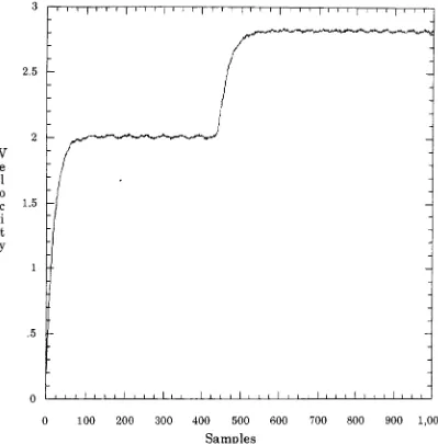
a

22% increase. Fig. #10 is

the

adaptive

controller witha

10

mSec

sampling

rate and

the

closed

loop

pole

is

set at

0.7.

The

closed

loop

poleat

0.7

was chosenas not

to

generate

high

gain values

in

the

poleplacement

feedback

controller.

As

shown

in

Fig.

#10,

there

is

very

little

overshoot

due

to the

closeapproximation of

the

closed

loop

pole

to the

error

in the velocity

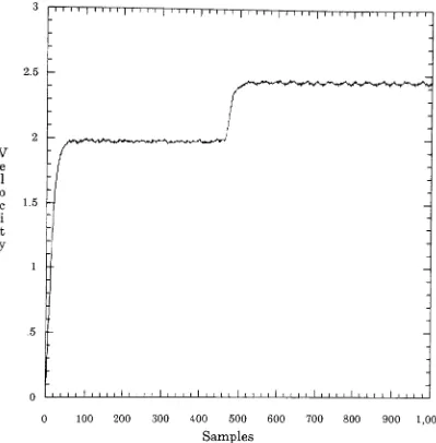
_{and slowconvergence.}

Fig.

#11 is

with

the

closed

loop

pole set at

0.5. In

this

figure

there

is

a

just

noticeable

increase in

the

overshoot

from Fig.

#10,

due

to

moving

the

closed

loop

pole

farther

away

from

the

open

loop

system

pole,

which causes

the

feedback

gains

to

increase

thus

driving

the

plant

harder. The increase

gain was

thought to

decrease

the

error

in the

output velocity.

In Figs. #10 &

#11,

the

10

mSec

sampling

rate cause errors

in

the

parameter estimation algorithm

producing

slow convergence and

large

steady

state errors

in

the

output velocity.

Fig.

#12

is

the

adaptivecontroller

with a

1

mSec

sampling

rate and

the

closed

loop

pole set at

0.7. In Fig.

#12 the

overshoot

due

to the

faster

sampling

rate

is

due

to the

positionof

the

open

loop

pole

being

closer

to the

unit circle

causing

a

37.5%

overshoot.

This high

overshoot shouldn't

be

a problem.

This figure

shows no

steady

state error

in

the

output velocity.

The

adaptation

is

complete

in approximately

115

samples,

which at

1

mSec

is 115

mSec.

Fig. #13

is the

response

to the

decrease

in torque

with

the

closed

loop

poleset at

0.9.

The

overshoot

is just

noticeably

lower,

but

still

high

at

35%.

Fig.

#13

shows

the

samezero

steady

state error

in

the

n I I I I I T

"1

i i i

|

i ' i

]

i i i prn i

|

i i i

p

i i i _| i i i

p

r

_1 I I 11 I I I I I L_Lj i i

I

i i i

Lj

i i

L

J I I LJ I L I 1 I I 1

0

100

200

300

400

500

600

700

800

900

1,000

Samples

[image:57.553.75.474.121.526.2]

2.5

V

e

1

o

c

i

t

y

1.5

' ' ' '

' ' ' ' '

I

' '

'I

' ' '

I

' ' ' i

|

i i i >

|

i i i i

|

i i i i

|

i i i i

|

i i i i

.5

i i i i i i ' ' i I i i i ' I i i i i I i i i i I i i i i I i i i i I i i i i l i i i i I

0 100

200

300

400

500

600

700

800

900

1,000

Samples

[image:58.553.75.474.118.524.2]

2.5

-2

-V

e

1

o

c

i

t

y

1.5

.5

-1 '

| ' '

|

i i i

|

i i i

|

i i i

|

t i i [

n i

|

i i i

p

r

_i_j i l_i i_ I i i i I i i i I ' i i I i ' i

I

i i i

I

i i i

I

i_ i i i i i

0

100

200

300

400

500

600

700

800

900

1,000 [image:59.553.74.474.105.521.2]

Samples

Figure #10:

Closed

Loop

Response

with

10

mSec

sampling

andclosed

loop

0

I

i i i

I

i i i

I

i i i

Lj

i i

I

i i i

I

i i i

L_i

i i I ' i i I i i i 1 i

0

100

200

300

400

500

600

700

800

900

1,000

Samples

Figure

#11: