Retrospective sampling in MCMC with an application to COM-Poisson regression

This is a repository copy of

Retrospective sampling in MCMC with an application to

COM-Poisson regression

.

White Rose Research Online URL for this paper:

http://eprints.whiterose.ac.uk/100012/

Version: Accepted Version

Article:

Chanialidis, Charalampos, Evers, Ludger, Neocleous, Tereza et al. (1 more author) (2014)

Retrospective sampling in MCMC with an application to COM-Poisson regression. Stat.

273 - 290. ISSN 2049-1573

https://doi.org/10.1002/sta4.61

Reuse

Items deposited in White Rose Research Online are protected by copyright, with all rights reserved unless indicated otherwise. They may be downloaded and/or printed for private study, or other acts as permitted by national copyright laws. The publisher or other rights holders may allow further reproduction and re-use of the full text version. This is indicated by the licence information on the White Rose Research Online record for the item.

Takedown

If you consider content in White Rose Research Online to be in breach of UK law, please notify us by

Retrospective sampling in MCMC with an

application to COM-Poisson regression

Charalampos Chanialidis*, Ludger Evers*, Tereza Neocleous *, and Agostino Nobile†

*_{School of Mathematics and Statistics, University of Glasgow}

†_{Department of Mathematics, University of York}

This refers to the pre-print version for the paper accepted in STAT. The post-print version can be foundhere.

Abstract

The normalisation constant in the distribution of a discrete ran-dom variable may not be available in closed form; in such cases the calculation of the likelihood can be computationally expensive. Ap-proximations of the likelihood or approximate Bayesian computation (ABC) methods can be used; but the resulting MCMC algorithm may not sample from the target of interest. In certain situations one can effi-ciently compute lower and upper bounds on the likelihood. As a result, the target density and the acceptance probability of the Metropolis-Hastings algorithm can be bounded. We propose an efficient and exact MCMC algorithm based on the idea of retrospective sampling. This procedure can be applied to a number of discrete distributions, one of which is the COM-Poisson distribution. In practice the bounds on the acceptance probability do not need to be particularly tight in order to accept or reject a move. We demonstrate this method using data on the emergency hospital admissions in Scotland in 2010, where the main interest lies in the estimation of the variability of admissions, since it is considered as a proxy for health inequalities.

1

Introduction

Bayesian and likelihood inference require the repeated evaluation of the like-lihood function, the probability (density) function π(y|θ) of the observed data y, regarded as a function of the model parameter θ. In some sam-pling models the function π(y|θ) is completely specified, in others it is only available up to a constant of proportionalityZ(θ), which must be taken into account when making inference about θ. We propose an MCMC algorithm which only makes use of cheaply computed, arbitrarily precise, upper and lower bounds on Z(θ). We consider in detail the case of the COM-Poisson distribution.

Approximating the normalisation constant with respect to the observed data can make MCMC methods inaccurate. Instead, we propose an MCMC scheme based on the idea of retrospective sampling: first draw the uni-form random variable U which is used to decide on the outcome of the Metropolis-Hastings acceptance/rejection move and then perform any calcu-lations needed on the acceptance ratio. Depending on the value of U, the acceptance ratio (which involvesZ both in the numerator and denominator) may not be needed to be known exactly.

The article is organised as follows. Sections2and 3present an overview of the COM-Poisson distribution and the basic idea behind the proposed retrospective sampling scheme. In Section4we describe a general approach to the construction of the bounds on Z(θ) for the case of discrete random variables. In Section5 we apply the method to data on hospital emergency admissions in Scotland, where identifying geographical areas with high vari-ance is the main interest since variation in admissions is a proxy for health inequalities. Concluding remarks can be found in Section6.

2

COM-Poisson distribution

The COM-Poisson distribution (Conway & Maxwell,1962) is a two-parameter generalisation of the Poisson distribution that allows for different levels of dispersion. The probability mass function of the COM-Poisson(λ,ν) distri-bution is

P(Y =y|λ, ν) = λ

y

(y!)ν

1

Z(λ, ν) y = 0,1,2, . . . (1)

forλ >0 andν≥0, whereZ(λ, ν) =

∞

X

j=0

λj

(j!)ν. The additional parameter ν

(ν <1) data. The Poisson distribution is a special case (ν= 1).

The normalisation constantZ(λ, ν) does not have a closed form (forν 6= 1) and has to be approximated, but can be upper bounded. An asymptotic approximation exists, which is reasonably accurate forλ >10ν _{(Minka et al.,} 2003).

Shmueli et al. (2005) describe methods for estimating the parameters of the COM-Poisson and show its flexibility in fitting count data compared to other distributions. They show that

E_[Y]≈λν1 + 1

2ν −

1

2,V[Y]≈

λ1ν

ν . (2)

This parametrisation of the COM-Poisson does not have a clear centering parameter, so we will use the reparametrisation µ = λν1 as proposed by Guikema & Coffelt(2008). The probability mass function is then

P(Y =y|µ, ν) =

µy

y!

ν

1

Z(µ, ν) y= 0,1,2, . . . (3)

withZ(µ, ν) =

∞

X

j=0

µj

j!

ν

. The mean and variance can be approximated by

E_[Y]≈µ+ 1

2ν −

1

2,V[Y]≈

µ

ν. (4)

Thus, in the new parametrisation µclosely approximates the mean, un-less both µ and ν are small. The mode of the distribution is ⌊µ⌋, as this formulation is just a tempered Poisson distribution.

The fact that Z(µ, ν), and thus the probability mass function P(Y =

y|µ, ν), is very expensive to compute, has been a key limiting factor for the use of the COM-Poisson distribution. In particular, in a Bayesian approach using the Metropolis-Hastings algorithm, each move requires an evaluation of Z(µ, ν) in order to compute the acceptance ratio. In Section 3 we will present an MCMC algorithm that does not need Z(µ, ν) to be computed exactly. In Section4we will then derive arbitrarily precise lower and upper bounds forZ(µ, ν).

3

Retrospective sampling

where π(θ) denotes the prior distibution of θ. In the Metropolis-Hastings algorithm a Markov chain is constructed in which, when the current state isθ, a candidate state θ∗ is drawn from a proposal distributionq(θ∗|θ) and then accepted with probabilitymin{1, p} with

p= π(y|θ

∗_)π(θ∗₎

π(y|θ)π(θ)

q(θ|θ∗)

q(θ∗_|θ). (5)

If θ∗ _{is rejected, the chain remains at the current state θ. In order to}

ac-cept the candidate θ∗ with probability min{1, p}, the acceptance ratio p is compared to a randomU ∼Unif(0,1)andθ∗ is accepted ifU < p. The key idea of the proposed algorithm is thatpneeds to be known exactly only if U

andpare very close. This requires exchanging the order of simulation. This idea, known as retrospective sampling, was first proposed by Papaspiliopou-los & Roberts (2008) as a way of sampling from a Dirichlet process. It has been used, amongst other things, for simulation of diffusion sample paths by

Beskos et al. (2006) and Sermaidis et al. (2013).

Suppose we have a sequence of increasingly and arbitrarily precise lower and upper bounds for π(y|θ), denoted by πˇ(y|θ) and πˆ(y|θ), respectively. Plugging these bounds into (5) yields lower and upper bounds for the accep-tance probability

ˇ

pn=

ˇ

πn(y|θ∗)π(θ∗)

ˆ

πn(y|θ)π(θ)

q(θ|θ∗₎

q(θ∗_|θ) pˆn=

ˆ

πn(y|θ∗)π(θ∗)

ˇ

πn(y|θ)π(θ)

q(θ|θ∗₎

q(θ∗_|θ) (6)

By construction pˇn ≤ p ≤ pˆn as well as pˇn → p and pˆn → p as n → ∞.

The proposed algorithm for deciding on the acceptance of θ∗ then proceeds as follows.

1. DrawU ∼Unif(0,1)and set the number of refinementsn= 0. 2. Computepˇn and pˆn and compare them toU.

• IfU ≤pˇn,accept the candidate value.

• IfU >pˆn,reject the candidate value.

• If pˇn < U < pˆn, refine the bounds, i.e increase n and return to

step 2.

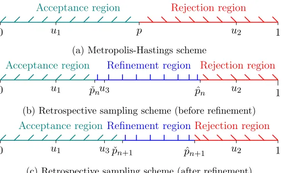
Figure 1 illustrates this idea. Panel 1a shows the Metropolis-Hastings strategy where p is the acceptance ratio and u1, u2 are two realizations of

the Unif(0,1) distribution. In the first case we accept the candidate value

acceptance and rejection regions can also be seen in the figure. Panel 1b

shows the retrospective sampling strategy along with the refinement region. When a realization of the Unif(0,1) falls into the refinement region (e.g.

u3), then in order to make a decision we have to refine the bounds. Panel1c

shows the new bounds, where the refined lower bound is aboveu3 and as a

result we accept the candidate valueθ∗.

Because the bounds pˇn and pˆn are arbitrarily tight, the algorithm will

eventually accept or reject a candidate valueθ∗.

4

Piecewise geometric bounds

This section explains how the bounds required in the previous algorithm can be constructed for discrete distributions with probability mass function given by

π(y|θ) =Z(θ)−1pθ(y), (7)

where the normalisation constantZ(θ) =P

ypθ(y)is not available in closed

form. The COM-Poisson distribution is an example of such a distribution. For ease of presentation we will assume that only computing the right tail is computationally challenging. At the end of the section we will explain how the method can be applied to bounding the left tail as well.

A simple way of reducing the computational burden is to compute the normalisation constantZ(θ) up to akth term and use this as a lower bound for Z(θ). An upper bound can be obtained by also considering an upper bound for the remaining terms. For the approach to be computationally efficient, kshould be chosen to be not too large, which in turn implies that the upper bound for the remaining terms will be rather loose.

On the other hand, if the ratio of consecutive probabilities is bounded by constants over a certain range ofy

ˇ

ay0,y1 ≤

pθ(y+ 1)

pθ(y)

≤aˆy0,y1, y∈ {y0, y0+ 1, . . . , y1−1}, (8)

then tighter bounds can be obtained, at little excess computationally cost. We will now construct bounds based on the constantsˇay0,y1,ˆay0,y1. These

tighter bounds are based on including piecewise bounds on a sequence of increasingly large blocks of probabilities in the tails. This corresponds to using the following lower bound and upper bound forZ(θ):

ˇ

whereE(θ) =Pk1

j=0pθ(j) is obtained by computing the sum of the first k1

terms exactly. Bˇ(θ)andBˆ(θ)are piecewise bounds on blocks of probabilities, computed as set out below. Rˆ(θ)is an upper bound on the remaining terms.

If (8) holds, then for allj ∈ {0, . . . , r}withr =y1−1−y0

(ˇay0,y1)

j _≤ pθ(y0+j)

pθ(y0)

= pθ(y0+ 1)

pθ(y0)

· · · pθ(y0+j)

pθ(y0+j−1)

≤(ˆay0,y1)

j_{. (9)}

We can rewrite the sum of the block of r+ 1probabilities as

r X

j=0

pθ(y0+j) =pθ(y0)

r X

j=0

pθ(y0+j)

pθ(y0)

. (10)

Taking advantage of (9) and (10) we obtain the bounds:

ˇ_by

0,y1(θ) =pθ(y0) r X

j=0

(ˇay0,y1) j _=p

θ(y0)

1−(ˇay0,y1) r+1

1−aˇy0,y1

≤

r X

j=0

pθ(y0+j)

ˆ_by

0,y1(θ) =pθ(y0) r X

j=0

(ˆay0,y1) j _=p

θ(y0)

1−(ˆay0,y1) r+1

1−aˆy0,y1

≥

r X

j=0

pθ(y0+j).

(11)

These bounds are computed in blocks of probabilities. Denote by s = (k1, . . . , kln) the sequence of end-points of the piecewise bounds, we then

define

ˇ

B(θ) =

ln−1 X

i=1

ˇ_bk

i,ki+1−1(θ), Bˆ(θ) = ln−1

X

i=1

ˆ_bk

i,ki+1−1(θ), (12)

which satisfiesBˇ(θ)≤

k_ln−1

P j=k1

pθ(j)≤Bˆ(θ). Finally, using the tail bound

ˆ

R(θ) = ˆbk_ln,∞(θ)≥ ∞

X

j=k_ln

pθ(j), (13)

we obtain the desired result that

ˇ

Z(θ) =E(θ) + ˇB(θ)≤

∞

X

j=0

pθ(j)≤E(θ) + ˆB(θ) + ˆR(θ) = ˆZ(θ) (14)

The previous bounds and the number of termsk1should haven, the number

the rest of the section we will assume that n is fixed. The bounds are in-creasingly tight as long ask1→ ∞. In practice the values ofk1 and kln are

chosen depending on θand the magnitude the previous contribution to the sum made. In our experience, choosingkssuch thatks+1−ks=dsford≈2

works well in practice.

So far we have set out how to compute bounds for the right tail of the distribution. If the mode of the distribution is large, then it is advisable to use the same strategy as above for the left tail too. The approach is essentially the same, with the main difference being that the bounds are computed right to left and that the summation will stop at0.

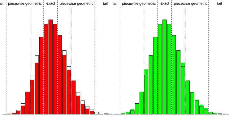
A graphical explanation of the procedure can be seen in Figure2 where the first two blocks are comprised of3 and5 probabilities respectively.

4.1 Bounds on the COM-Poisson normalisation constant

In the COM-Poisson case, the bounds in (8) and (11) are

ˇ

ay0,y1 =

µ y1

ν

, ˆay0,y1 =

µ y0+ 1

ν

, (15)

for y0, y1 >⌊µ⌋ and

ˇ_by

0,y1(θ) =p(y0)

µ y1

ν 1−

µr yr 1

ν

1−_yµ

1

ν, ˆby0,y1(θ) =p(y0)

µ y0+ 1

ν 1−

µr

(y0+1)r ν

1−_yµ

0+1 ν ,

(16) wherer=y1−1−y0 andp(y0) =

µy0

y0! ν

is the unnormalised density of the COM-Poisson. Bounds for the left tail of the distribution are computed in a similar way.

4.2 Weighted Poisson distributions

Del Castillo & Pérez-Casany (1998) developed a family of distributions, known as weighted Poisson distributions, that can handle both under- and overdispersion. A random variableY is defined to have a weighted Poisson distribution if its probability mass function can be written as

P(Y =y) =e−λλ

y_w y

W y! y= 0,1,2, . . . (17)

whereW =e−λ

∞

X

j=0

λjwj

j! . The weight function is defined as wy = (y+a)

r

These distributions are used for modelling data with partial recording: when the event Y = y occurs, a Poisson variable is recorded with probability proportional towy.

The bounds, found in (8), for this distribution forr >0are

ˇ

ay0,y1 = λ y1

wy1 wy1−1

, ˆay0,y1 = λ y0+ 1

wy0+1 wy0

. (18)

Similar bounds can be constructed forr <0.

5

Application on emergency hospital admissions in

Scotland

As an illustration of the method, we consider data on the hospital emer-gency admissions for each intermediate geography (1235 in total) in Scot-land for the year 2010. Scotland is divided into 6505 small areas, called datazones, each containing around350households. An intermediate geogra-phy is comprised of neighbouring datazones. The Scottish Index of Multiple Deprivation (SIMD) is the Scottish government’s official tool for identifying datazones suffering from deprivation. This index provides a relative ranking for each datazone, from 1 (most deprived) to 6505 (least deprived). The Scottish government’s cut-off for a datazone to be considered deprived is to belong in the 15% most deprived datazones in Scotland. Using the SIMD ranks for areas larger than datazones (such as intermediate geographies) one can consider the percentage of datazones within that intermediate geogra-phy that are in the 15% most deprived e.g. if an intermediate geography is comprised of 20 datazones and 10 of them are in the 15% most deprived then its local share is 50%. This can also be applied in larger areas such as local authorities.

to the small number of intermediate geographies they are comprised of and not because they are considered to be affluent areas.

This approach, of using a cut-off point for the datazones, has its draw-backs since datazones that just miss the 15% cut-off point are treated the same as the ones that are far away from it. A better approach, and the one followed in this paper, would be to weight every datazone and average over all the datazones that belong to the same intermediate geography. Datazones with a small SIMD rank (most deprived) will have a higher weight and each datazone’s SIMD rank contributes for the deprivation of the intermediate geography they belong to.

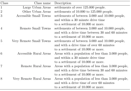
The Scottish Government classifies urban and rural areas across Scotland based on two criteria: population and accessibility to areas of contiguous high population density postcodes (that make up what is known as a settlement). The joint classification can be seen in table3. Using this classification as an ordinal covariate is not appropriate due to how it is coded. For example the

6th class (accessible rural area) is closer to an urban area than the previous two. Instead, we will use as covariates the percentages of those classes within each intermediate geography, e.g. if an intermediate geography is comprised of6datazones where3of them are coded as large urban areas and the other

3 as accessible small towns, the percentages of the first and the third class will be 50% and 0% for all the other classes. For ease of interpretation we center all covariates.

5.1 Regression model and results

Sellers & Shmueli(2010) propose a COM-Poisson regression model based on the(λ, ν)formulation whereasGuikema & Coffelt(2008) prefer to work with the (µ, ν) reformulation. Modifying the latter model we take into account the population and age structure of each intermediate geography and include expected counts (Ei) of hospital emergency admissions for each intermediate

is specified as follows

P(Yi=yi|µi, νi) =

µyi i

yi! νi

1

Z(µi, νi)

,

Z(µi, νi) =

∞

X

j=0

µj_i j!

!νi ,

log µi

Ei

=x⊺

iβ+φi ⇒E[Yi]≈Eiexp{x⊺iβ+φi},

logνi=−x⊺_ic ⇒V[Yi]≈Eiexp{x⊺_iβ+φi+x⊺_ic}. (19)

Y is the dependent random variable being modelled (emergency hospi-tal admissions), Ei is the expected emergency hospital admissions for the

i intermediate geography, φi are the random effects for the parameter µ,

while β and c are the regression coefficients for the centering link function and the shape link function. Finally, the covariates xi are comprised of:

the deprivation weight of the intermediate geography i, the percentages of each urban/rural class within the intermediate geographyi (using large ur-ban areas as the baseline model), and 32 dummy variables that relate the intermediate geographyito its local authority.

The CAR prior being used for the random effectsφiin this model is given

by

φk|φ−k∼N(

ρPn

i=1wkiφi

ρPn

i=1wki+ 1−ρ

, τ

2

ρPn

i=1wki+ 1−ρ

) (20)

and was proposed by Leroux et al. (2000) for modelling varying strengths of spatial autocorrelation. It can be seen as a generalisation ofBesag et al.

(1991) CAR prior where the first model can only represent strong spatial autocorrelation and produces smooth random effects. The random effects for non-neighbouring areas are conditionally independent given the values of the random effects of all the other areas. The parameter ρ can be seen as a spatial autocorrelation parameter, with ρ = 0 corresponding to indepen-dence, whileρ= 1corresponds to strong spatial autocorrelation. In the first case there is an absence of spatial correlation in the data and the overdisper-sion is not caused by a spatial heterogeneity while in the second case all the overdispersion is due to the spatial autocorrelation. When 0 < ρ < 1, the random effects are correlated and the data present a combination of spatial structured and unstructured components. Lee (2011) compares four of the most common CAR models and concludes that the model byLeroux et al.

Larger values ofβ andc can be translated to higher mean and higher vari-ance for the response variable. We implement a Bayesian approach for the previous model, and propose an efficient and exact MCMC algorithm based on the piecewise geometric bounds and the retrospective sampling algorithm. We use noninformative multivariate normal priors for the regression coeffi-cients with a mean of zero and a variance of 106_{. A uniform prior on the}

unit interval is specified for ρ, and a uniform prior on the interval (0,1000)

is adopted forτ2. In addition, the proposal distribution q is chosen to be a multivariate normal centered at the current value. Thus, the second ratio in (5) cancels out due to the symmetry of the multivariate normal distribution. This algorithm is known as a random walk Metropolis-Hastings.

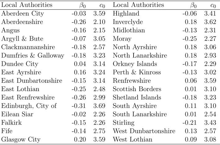
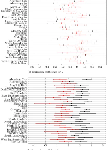
Table 4 shows the non-model-based regression coefficients for each lo-cal authority (32 local authorities in total). These coefficients refer to the intercepts of the 32 regression models (one for each local authority) where the offset (e.g. logEi) is the only covariate. It must be noted that some of

the local authorities were comprised of a small number of data points, for example Orkney Islands, Shetland Islands, and Eilean Siar include less than

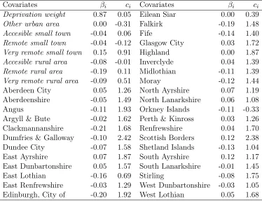
10 intermediate geographies. Table 5 shows the regression coefficients for the model in (19). The COM-Poisson coefficients for ν of most covariates are positive which is a sign of overdispersion. Table 5 shows that there is a wide range of values for the coefficients c. They can take negative values (Orkney Islands) and up to greater than 2 (Dumfries & Galloway, Scot-tish Borders). The regression coefficients b1, c1 for the deprivation weights

have positive posterior median estimates, 0.87 and 0.05 respectively, with

(0.84,0.90)and(−0.36,0.52)as their95%credible intervals. This translates to higher emergency hospital admissions for intermediate geographies with high deprivation. This is not true for the variance, since the credible interval includes negative values. The data have a strong spatial autocorrelation as can be seen, in Table 6, from the credible intervals of the autocorrelation parameterρ.

large µ coefficients (corresponding to poor health) do not necessarily have large ν coefficients (corresponding to large health inequalities). This can be seen in local authorities such as North Ayrshire, North Lanarkshire and South Ayrshire.

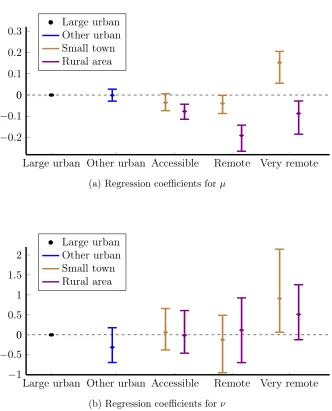
The coefficients for the percentages of each class can be seen in Figure

4 where large urban areas are considered to be the baseline model. The remaining classes are plotted with regards to their distance from an urban area. The black circle represents the large urban area class whereas the blue, brown and violet lines represent the urban area, small town and rural area classes respectively. It can be seen that very remote small towns have higher (on average) emergency hospital admissions (see Panel4a) and higher variance (see Panel4b) compared to large urban areas.

Finally, Figure 5 shows the standardised incidence ratio of the average emergency hospital admissions using the non-model-based coefficients (on the left) and the coefficients of the full model (on the right).

R (R Core Team,2014) was used for all the computations in this paper. Traceplots, density plots, autocorrelation plots (for every regression coeffi-cient) and results for the Gelman and Rubin diagnostic, (Gelman & Rubin,

1992), were employed to assess convergence of the MCMC sampler to the posterior distribution, using the coda package (Plummer et al.,2006).

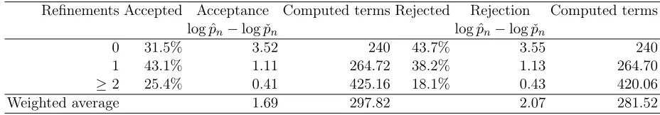
5.2 Range of bounds for the acceptance probability

The computational speed of the proposed technique depends on which strat-egy is chosen to refine the bounds. We chose to increase the number of terms that are computed exactly for the estimation of the normalisation constant and use the piecewise geometric bounds for the remaining terms. We start by computing exactly 240terms for everyZ(µi, νi) and every time the bounds

weighted average for the log difference of the bounds when the MCMC re-jects the candidate value for the first parameter is 2.51 which means that a rejection decision can often be reached with very loose upper and lower bounds.

6

Conclusion

In this paper we have focused on the problem of computing the normalising constant in the probability mass function of a discrete random variable, when it is not available in closed form and its computation is demanding. We have shown that if the ratios of consecutive probabilities can be bounded over ranges of the random variable, lower and upper bounds on the normalising constant can be derived, leading to an exact and fast MCMC algorithm in a Bayesian inferential setting. Furthermore, the results show that in order for the MCMC algorithm to make a decision between accepting or rejecting a candidate move, the approximation of the bounds of the acceptance prob-ability does not need to be precise. We applied this method to emergency hospital admissions data in Scotland, using the COM-Poisson distribution. We concentrated on the COM-Poisson distribution, a very flexible general-isation of the Poisson distribution, since it allows modelling the mean and the variance explicitly. As a result, we were able to identify areas with a high level of health inequalities.

7

Acknowledgements

We would like to thank Peter Craigmile, Chris Holmes, Dirk Husmeier, and Duncan Lee for their helpful comments.

References

Besag, J, York, J & Mollié, A (1991), ‘Bayesian image restoration, with two applications in spatial statistics,’ Annals of the Institute of Statistical Mathematics,43(1), pp. 1–20, doi:10.1007/BF00116466.

Bivand, R (2014), spdep: Spatial dependence: weighting schemes, statistics and models, r package version 0.5-71.

Bivand, R & Lewin-Koh, N (2013),maptools: Tools for reading and handling spatial objects, r package version 0.8-27.

Conway, RW & Maxwell, WL (1962), ‘A queuing model with state dependent service rate,’Journal of Industrial Engineering,12, pp. 132–136.

Del Castillo, J & Pérez-Casany, M (1998), ‘Weighted poisson distribu-tions for overdispersion and underdispersion situadistribu-tions,’ Annals of the Institute of Statistical Mathematics, 50(3), pp. 567–585, doi:10.1023/A: 1003585714207.

Eddelbuettel, D & François, R (2011), ‘Rcpp: Seamless R and C++ integra-tion,’Journal of Statistical Software,40(8), pp. 1–18.

Gelman, A & Rubin, DB (1992), ‘Inference from iterative simulation using multiple sequences.’ Statistical Science,7(4), pp. 457–472.

Guikema, SD & Coffelt, JP (2008), ‘A flexible count data regression model for risk analysis.’ Risk analysis: an official publication of the Society for Risk Analysis,28, pp. 213–223, doi:10.1111/j.1539-6924.2008.01014.x.

Lee, D (2011), ‘A comparison of conditional autoregressive models used in Bayesian disease mapping.’ Spatial and Spatio-temporal Epidemiology,

2(2), pp. 79–89.

Lee, D (2013), ‘CARBayes: An R package for Bayesian spatial modeling with conditional autoregressive priors,’ Journal of Statistical Software, 55(13), pp. 1–24.

Leroux, B, Lei, X & Breslow, N (2000), ‘Estimation of disease rates in small areas: A new mixed model for spatial dependence,’ in Halloran, M & Berry, D (eds.),Statistical Models in Epidemiology, the Environment, and Clini-cal Trials, Springer New York, vol. 116 ofThe IMA Volumes in Mathemat-ics and its Applications, pp. 179–191, doi:10.1007/978-1-4612-1284-3_4.

Minka, TP, Shmueli, G, Kadane, JB, Borle, S & Boatwright, P (2003), ‘Com-puting with the COM-Poisson distribution,’ Tech. rep., CMU Statistics Department.

Papaspiliopoulos, O & Roberts, GO (2008), ‘Retrospective Markov chain Monte Carlo methods for Dirichlet process hierarchical models,’

Plummer, M, Best, N, Cowles, K & Vines, K (2006), ‘Coda: Convergence diagnostics and output analysis for mcmc,’R News,6(1), pp. 7–11.

R Core Team (2014),R: A Language and Environment for Statistical Com-puting, R Foundation for Statistical Computing, Vienna, Austria, ISBN 3-900051-07-0.

Scottish Government (2009), ‘Scottish index of multiple deprivation,’ doi: http://dx.doi.org/10.5255/UKDA-SN-6871-1.

Sellers, KF & Shmueli, G (2010), ‘A flexible regression model for count data,’

Annals of Applied Statistics,4(2), pp. 943–961, doi:10.1214/09-aoas306.

Sermaidis, G, Papaspiliopoulos, O, Roberts, GO, Beskos, A & Fearn-head, P (2013), ‘Markov chain Monte Carlo for exact inference for dif-fusions,’ Scandinavian Journal of Statistics, 40(2), pp. 294–321, doi: 10.1111/j.1467-9469.2012.00812.x.

0 u1 p u2 1

Acceptance region Rejection region

(a) Metropolis-Hastings scheme

0 u1 pˇnu3 pˆn u2 1 Acceptance region Refinement region Rejection region

(b) Retrospective sampling scheme (before refinement)

0 u1 u3pˇn+1 pˆn+1 u2 1

Acceptance region Refinement regionRejection region

(c) Retrospective sampling scheme (after refinement)

exact

tail piecewise geometric piecewise geometric tail tail piecewise geometric exact piecewise geometric tail

Table 1: The local share considers the percentage of a local authority’s datazones that are amongst the15% most deprived in Scotland.

Local Authorities Local Share Local Authorities Local Share Aberdeen City 10.49 Highland 5.48 Aberdeenshire 1.33 Inverclyde 38.18

Angus 4.23 Midlothian 3.57

Argyll & Bute 8.20 Moray 0.86 Clackmannanshire 18.75 North Ayrshire 24.02 Dumfries & Galloway 5.70 North Lanarkshire 21.29 Dundee City 30.17 Orkney Islands 0.00 East Ayrshire 17.53 Perth & Kinross 3.43 East Dunbartonshire 3.15 Renfrewshire 20.09 East Lothian 2.50 Scottish Borders 3.85 East Renfrewshire 4.17 Shetland Islands 0.00 Edinburgh, City of 10.93 South Ayrshire 12.24 Eilean Siar 0.00 South Lanarkshire 14.57

Falkirk 8.63 Stirling 6.36

Table 2: The local share considers the percentage of a local authority’s datazones that are amongst the15% least deprived in Scotland.

Local Authorities Local Share Local Authorities Local Share Aberdeen City 35.58 Highland 4.79 Aberdeenshire 21.93 Inverclyde 2.73

Angus 9.86 Midlothian 14.29

Argyll & Bute 4.10 Moray 8.62 Clackmannanshire 9.38 North Ayrshire 2.79 Dumfries & Galloway 4.15 North Lanarkshire 6.22 Dundee City 11.17 Orkney Islands 0.00 East Ayrshire 6.49 Perth & Kinross 12.57 East Dunbartonshire 47.24 Renfrewshire 17.76 East Lothian 18.33 Scottish Borders 4.62 East Renfrewshire 57.50 Shetland Islands 0.00 Edinburgh, City of 39.53 South Ayrshire 16.33 Eilean Siar 0.00 South Lanarkshire 12.31

Falkirk 13.20 Stirling 18.18

Table 3: Scottish Government joint Urban/Rural Classification.

Class Class name Description

1 Large Urban Areas settlements of over125.000people. 2 Other Urban Areas settlements of10.000to125.000people.

3 Accessible Small Towns settlements of between 3.000and 10.000people, and within a30 minute drive time

to a settlement of10.000or more.

4 Remote Small Towns settlements of between 3.000and 10.000people, and with a drive time between30 and 60 minutes to a settlement of10.000or more.

5 Very Remote Small Towns settlements of between3.000and 10.000people, and with a drive time of over60 minutes

to a settlement of10.000or more.

6 Accessible Rural Areas Areas with a population of less than3.000people, and within a30 minute drive time

to a settlement of10.000or more.

7 Remote Rural Areas Areas with a population of less than3.000people, and with a drive time between30 and 60 minutes to a settlement of10.000or more.

8 Very Remote Rural Areas Areas with a population of less than3.000people, and with a drive time of over60 minutes

Table 4: Posterior medians of the non-model-based regression coefficients for each local authority.

Local Authorities β0 c0 Local Authorities β0 c0

Table 5: Posterior medians for the regression coefficients of the full model.

Covariates βi ci Covariates βi ci Deprivation weight 0.87 0.05 Eilean Siar 0.00 0.39

Other urban area 0.00 -0.31 Falkirk -0.19 1.48

Accesible small town -0.04 0.06 Fife -0.14 1.40

Remote small town -0.04 -0.12 Glasgow City 0.03 1.72

Very remote small town 0.15 0.91 Highland 0.00 1.87

Accesible rural area -0.08 -0.01 Inverclyde 0.04 1.39

Remote rural area -0.19 0.11 Midlothian -0.11 1.39

Very remote rural area -0.09 0.51 Moray -0.12 1.44 Aberdeen City 0.05 1.26 North Ayrshire 0.07 1.19 Aberdeenshire -0.05 1.49 North Lanarkshire 0.06 1.08 Angus -0.11 1.93 Orkney Islands -0.11 -0.33 Argyll & Bute -0.02 1.62 Perth & Kinross 0.03 1.26 Clackmannanshire -0.21 1.68 Renfrewshire 0.04 1.70 Dumfries & Galloway -0.10 2.42 Scottish Borders 0.12 2.38 Dundee City -0.07 1.58 Shetland Islands -0.13 1.04 East Ayrshire 0.07 1.87 South Ayrshire 0.12 1.17 East Dunbartonshire 0.05 1.57 South Lanarkshire -0.01 1.45 East Lothian -0.16 0.69 Stirling -0.08 1.75 East Renfrewshire -0.03 1.29 West Dunbartonshire -0.03 1.05 Edinburgh, City of -0.20 1.92 West Lothian 0.05 1.68

Table 6: Posterior medians for the variance and spatial autocorrelation of the random effects.

Median 2.5% 97.5%

τ2 0.004 0.002 0.008

Table 7: Percentages for refinements when updating the parameter µ.

Refinements Accepted Rejected Still need refinement

0 9.6% 43.2% 47.2%

1 11.5% 20.1% 15.6%

≥2 7.3% 8.3% 0%

Total 28.4% 71.6%

Table 8: Percentages for refinements when updating the parameterν.

Refinements Accepted Rejected Still need refinement

0 11.9% 27.2% 60.9%

1 16.3% 23.8% 20.8%

≥2 9.6% 11.2% 0%

Total 37.8% 62.2%

Table 9: Mean values for the difference of the log bounds and the computed terms when updating the parameterµ.

Refinements Accepted Acceptance Computed terms Rejected Rejection Computed terms log ˆpn−log ˇpn log ˆpn−log ˇpn

0 33.9% 3.51 240 60.3% 3.55 240

1 40.5% 1.11 264.71 28.1% 1.13 264.66

≥2 25.6% 0.40 426.15 11.6% 0.43 420.55

Weighted average 1.74 297.84 2.51 267.75

Table 10: Mean values for the difference of the log bounds and the computed terms when updating the parameterν.

Refinements Accepted Acceptance Computed terms Rejected Rejection Computed terms log ˆpn−log ˇpn log ˆpn−log ˇpn

0 31.5% 3.52 240 43.7% 3.55 240

1 43.1% 1.11 264.72 38.2% 1.13 264.70

≥2 25.4% 0.41 425.16 18.1% 0.43 420.06

−0.6 −0.5 −0.4 −0.3 −0.2 −0.1 0 0.1 0.2 0.3

Aberdeen City Aberdeenshire Angus Argyll & Bute Clackmannanshire Dumfries & Galloway Dundee City East Ayrshire East Dunbartonshire East Lothian East Renfrewshire Edinburgh City of Eilean Siar Falkirk Fife Glasgow City Highland Inverclyde Midlothian Moray North Ayrshire North Lanarkshire Orkney Islands Perth & Kinross Renfrewshire Scottish Borders Shetland Islands South Ayrshire South Lanarkshire Stirling West Dunbartonshire West Lothian 0

(a) Regression coefficients forµ

−1 0 1 2 3 4 5

Aberdeen City Aberdeenshire Angus Argyll & Bute Clackmannanshire Dumfries & Galloway Dundee City East Ayrshire East Dunbartonshire East Lothian East Renfrewshire Edinburgh City of Eilean Siar Falkirk Fife Glasgow City Highland Inverclyde Midlothian Moray North Ayrshire North Lanarkshire Orkney Islands Perth & Kinross Renfrewshire Scottish Borders Shetland Islands South Ayrshire South Lanarkshire Stirling West Dunbartonshire West Lothian 0

(b) Regression coefficients forν

Figure 3: Credible intervals for the regression coefficients of the local au-thorities. The non-model-based regression coefficients of table 4 are shown

Large urban Other urban Accessible Remote Very remote

−0.2

−0.1 0 0.1 0.2 0.3

0

Large urban Other urban Small town Rural area

(a) Regression coefficients forµ

Large urban Other urban Accessible Remote Very remote

−1

−0.5 0 0.5 1 1.5 2

0

Large urban Other urban Small town Rural area

(b) Regression coefficients forν

Non−model−adjusted

0.0 0.5 1.0 1.5 2.0 2.5

Glasgow Edinburgh

Model−adjusted

0.0 0.5 1.0 1.5 2.0 2.5

Glasgow Edinburgh