An iterative orthogonal forward regression algorithm

This is a repository copy of

An iterative orthogonal forward regression algorithm

.

White Rose Research Online URL for this paper:

http://eprints.whiterose.ac.uk/107315/

Version: Accepted Version

Article:

Guo, Y., Guo, L. Z., Billings, S. A. et al. (1 more author) (2015) An iterative orthogonal

forward regression algorithm. International Journal of Systems Science, 46 (5). pp.

776-789. ISSN 0020-7721

https://doi.org/10.1080/00207721.2014.981237

[email protected] https://eprints.whiterose.ac.uk/

Reuse

Unless indicated otherwise, fulltext items are protected by copyright with all rights reserved. The copyright exception in section 29 of the Copyright, Designs and Patents Act 1988 allows the making of a single copy solely for the purpose of non-commercial research or private study within the limits of fair dealing. The publisher or other rights-holder may allow further reproduction and re-use of this version - refer to the White Rose Research Online record for this item. Where records identify the publisher as the copyright holder, users can verify any specific terms of use on the publisher’s website.

Takedown

If you consider content in White Rose Research Online to be in breach of UK law, please notify us by

1

An Iterative Orthogonal Forward Regression Algorithm

Revised on 02/10/2014

Revised on 23/07/2014

Yuzhu Guo, L.Z. Guo, S. A. Billings, and Hua-Liang Wei

Department of Automatic Control and Systems Engineering,

The University of Sheffield, Mappin Street, Sheffield, S1 3JD, UK

Abstract -- A novel iterative learning algorithm is proposed to improve the classic orthogonal forward

regression (OFR) algorithm in an attempt to produce an optimal solution under a purely OFR

framework without using any other auxiliary algorithms. The new algorithm searches for the optimal

solution on a global solution space while maintaining the advantage of simplicity and computational

efficiency. Both a theoretical analysis and simulations demonstrate the validity of the new algorithm.

Index Terms: Iterative orthogonal forward regression, model structure detection, nonlinear system

identification, orthogonal least squares

1. Introduction

The NARMAX (Nonlinear AutoRegressive Moving Average with eXogenous input) model and the

associated Orthogonal Forward Regression (OFR) algorithm have been widely applied in nonlinear

system identification including in the modelling of many engineering, chemical, biological, medical,

geographical, and economic systems (Billings 2013). Variations of these algorithms have been

developed for lumped and distributed parameter systems, time-invariant and rapidly time-varying

systems, in the time, frequency and spatio-temporal domains. The OFR algorithm, which is also

known as the OLS (Orthogonal Least Squares) or the FOLSR (Forward Orthogonal Least Squares

Regression) algorithm, determines the model structure of nonlinear systems based on the ERR (Error

Reduction Ratio) criterion without any a priori knowledge except for the specification of an initial

model set.

However, under some extreme circumstances (for example non-persistently exciting inputs) the

2

Mao and Billings 1997; Piroddi and Spinelli 2003; Sherstinsky and Picard 1996). Solutions are

available which solve this problem (Billings 2013; Billings and Wei 2007; Li et al. 2006; Mao and

Billings 1997; Wei and Billings 2008) but most of these methods involve combining the OFR

algorithm with other routines. Contrary to the earlier approaches, this paper presents a new proposal

to enhance the classic OFR without making any major conceptual changes. To clarify the difference

with a standard OFR algorithm the new algorithm will be referred to as the iterative Orthogonal

Forward Regression (iOFR) algorithm. The core ideas of the new algorithm are presented and it is

shown that the new iOFR method can produce an optimal model under a revised but purely OFR-ERR

framework. Another advantage of the new iOFR algorithm is that the new two-step iOFR does not

require the initial model obtained at the first step to be an accurate model, which is different from

most coarse-to-fine algorithms. This means the iOFR algorithm can start from an incomplete model

and can still produce a complete optimal model.

The remainder of the paper is organised as follows. Section 2 briefly reviews the classic OFR

algorithm. Section 3 introduces the new iterative OFR algorithm. A simple example is initially

introduced to motivate the introduction of an iterative process to search for the optimal solution on a

global solution space rather than a local space. Three illustrative examples are discussed in section 4.

The first example shows that the iOFR can successfully eliminate any redundant terms and obtain a

parsimonious model. The second example shows how the new iOFR algorithm can find the correct

terms which may have been missed in earlier algorithms. The third example is used to illustrate the

identification of the NARMAX model with noise terms using the new iOFR algorithm. Conclusions

3

2. NARMAX model and orthogonal forward regression

2.1 NARMAX model

A NARMAX model is essentially an expansion of the output with past inputs, outputs and noise terms.

A wide class of nonlinear systems can be represented by a NARMAX model (Billings 2013;

Leontaritis and Billings 1985) which can be defined as

 



 









 





 

 







 

1 , 2 , , , , 1 ,

, , 1 , 2 , ,

y

u e

y k y k y k n u k d u k d

y k F e k

u k d n e k e k e k n

       

 

 

 _{    } 

 

(1)

where y(k), u(k) and e(k) are the system output, input, and noise sequences respectively; ny, nu, and ne

are the maximum lags for the system output, input, and noise; F( ) is some nonlinear function; d is a

time delay which is often set as d=1. Although both Volterra series and NARMAX models represent

input-output relations, the Volterra series give an explicit representation while the NARMAX model

gives an implicit representation, which is often of a much more compact form. A large class of

systems can be described using the NARMAX model by selecting different forms of the functions F ,

for example the nonlinear DARX model (Shouche et al. 1998).

2.2 OFR algorithm

System identification based on the NARMAX model involves selecting the significant model terms

from a full candidate term dictionary and then estimating the associated parameters in order to build a

parsimonious model. The search for model subsets with minimum mean square error (MSE) can be

approached in a straightforward manner by computing all possible regressions but the amount of

computation required can be formidable, because the number of possible subsets increases

exponentially. OFR offers an efficient procedure for finding the best subsets (Billings et al. 1989;

Billings et al. 1988). The OFR algorithm involves a stepwise orthogonalisation of the regressors and a

forward selection of the model terms based on the error reduction ratio (ERR) criterion (Billings

4

Specify an initial full model set D





candidate terms. Terms i are linear or nonlinear functions of the input, output and noise. When the

measurements of input, output, and noise are available, these functions can be evaluated and

represented as the regression matrix





    (2)

where the column vectors i's are defined as





T i i i N

 . By slightly abusing the notation,

we sometimes use the column vector i to represent term i and the regression matrix which includes

all the columns to represent the term dictionary D in later discussions.

Because normally there is a lack of knowledge regarding the structure of function F in (1), the term

dictionary is selected to be redundant and it is assumed that F can be expressed as a linear

combination of a subset of D, that is





s   s s s 

D D, where s_i





model of system (1) can be represented by basis functions

 

 

1

( )

s i

s i i

y t t e t



 







where _i are the coefficients.

Hence system identification based on the measurements involves the determination of the model

structure and the estimation of the parameters. However the determination of the structure and the

estimation of the parameters are coupled with each other. The significance of a term in a model

depends on the estimated parameters while the estimation of the coefficients depends on the model

structure. Using a traditional forward regression algorithm, all the coefficients in a model need to be

re-estimated when a new term is added. Hence the evaluation of the contribution of a newly added

term to the model is computationally intensive because of the matrix inversion involved in the

coefficient re-estimation. However, the structure detection and the parameter estimation can be

5

Data collected from 1 to N yields the matrix form of equation (3)

.

s

 

y (4)

An orthogonal decomposition of s is given as

s WA (5)

Here A is a  s s unit upper triangular matrix and

1 s

 

  

W w w (6)

is a N matrix with orthogonal columns which satisfy

0, ,

0,

i i j

d i j

i j

  

  _ 

w w (7)

where  , denotes the inner product defined on space N

R , that is

1

, ( ) ( )

N T

i j i j i j

k

w k w k



 



w w w w .

Equation (4) can then be written as

1 i i i g    



y Wg w  (8)

The coefficient of each term gi can be calculated individually as

, . , i i i i

g  w y

w w (9)

In the OFR algorithm a criterion called the error reduction ratio (ERR) has been introduced to

measure the significance of the model terms in the description of system (1) and to determine the

model structure by selecting all the significant terms. The error reduction ratio ERRi due to term wi is

defined as 2 2 , , , , , ,

i i i i

i

i i

g

ERR  w w  w y

6

It is worth noting that the ERR criterion evaluates the contribution of a term considering both the form

of the term and also the associated coefficients, which is essentially different from the orthogonal

projection or inner product criterion used by the Projection Pursuit and Matching Pursuit algorithms

(Huber 1985; Mallat and Zhang 1993; Pati et al. 1993), where the effects of the coefficients has not

been considered.

When all the terms are orthogonal with each other the values of ERR of the terms in a model satisfy

1

, 1

,

s

i i

ERR









y y (11)

where the last term on the right hand side of the equation represents the noise-to-signal ratio.

The error reduction ratio offers a simple, effective, and intuitive means of selecting a subset of

significant terms from a large number of candidate terms in a forward regression manner. By applying

the OFR algorithm and the ERR criterion, the contribution of a term can be evaluated avoiding

re-estimating all the coefficients. At each step, a term which produces the largest value of ERRi among

the candidate terms is selected, and the selection procedure is terminated at s step when

1

1

s

i i

ERR











where  is a desired tolerance, and this leads to a subset model of s terms. In the application of the

OFR-ERR algorithm, various criteria, such as AIC (Akaike Information Criterion), BIC (Bayesian

Information Criterion), and other statistical tests, can be used to aid the termination of the term

selection (Billings and Chen 1989).

To summarise, the standard orthogonal forward regression algorithm consists of the following steps:

(i) Sufficiently excite the system and measure the inputs and outputs of the system;

(ii) Specify an initial full model set of candidate terms and the value of  ;

(iii) Compute the values of the ERR for each of the  candidate terms and select the term which

7

(iv) At the kth (k2 ) stages compute the values of the error reduction ratio for each of the

( k 1) remaining candidate terms by assuming that each is the kth term in the selected model and

perform the corresponding orthogonalisation; The term that gives the largest value of the error

reduction ratio is then selected into the model as the kth term. If condition (12) is satisfied, finish the

process and go to (v). Otherwise set k k 1 and repeat step (iv);

(v) The final model contains s terms and the parameter estimates can be calculated using a least

squares formulae.

A geometric interpretation of the above procedure has been given by Chen, Billings & Luo (1989).

Consider y as a vector in the N dimensional Euclidean space N

R where

 

independent vectors in this space. Each of the vectors can be spanned into a one dimensional subspace

of N

R . Denote the subspace which is spanned by _i as S

 

measure the orthogonal projections of y onto each of the subspaces. The subspace

 

s

S  which gives

the maximal projection is determined and the corresponding term 1

s

 is selected as the first term

which is denoted as w1. At the second step, consider the orthogonal projections of y onto a two

dimensional space

 

s i

S which is spanned by 1

s

 and each of the remaining (1) vectors i

where i



  

projection of y onto

 

s i

S can be determined by evaluating the orthogonal projection of y onto wi.

The term 2

s

 which spans the subspace





s s

S on which the orthogonal projection of y reaches the

maximum is selected as the second term. The orthogonalised vectors





basis of the subspace





s s

S . At the kth step, the orthogonal projections of y onto k-dimensional

subspaces are considered. The selected term k

s

 and the previous k-1 terms span the subspace





8

Compared to traditional forward regression methods, the OFR algorithm is computationally efficient

because it successfully avoids the re-estimation of the parameters and evaluates the contribution of

each term individually. The OFR is also extremely sufficient in the term selection. At the kth step the

regression analysis are preformed on the orthogonal complement of the subspace spanned by the

previous k-1 terms. This successfully eliminates the information redundancy in the model and

produces a parsimonious model. Accordingly, the OFR can in most cases obtain the optimal solution

with only forward selection rather than stepwise regression. However, the classic OFR algorithm may

occasionally give a suboptimal model because of the information overlap among the nonorthogonal

terms. For example, a wrong term can be selected at the first step because the term carries the

information from more than one correct term. This often happens at the first step because the terms

have not been orthogonalised. In this paper, a new iterative OFR algorithm will be introduced to solve

this problem, to improve the performance of the classic OFR algorithm, and to provide a relatively

simple and easy to use algorithm for term selection in complex dynamic models.

3. Iterative orthogonal forward regression

Following the discussion in the previous section, the OFR algorithm selects at each step the best term

which comprises an optimal subspace with the existing terms. However optimal choices at every step

cannot always guarantee a global optimum. Although the classic OFR algorithm is always very

efficient, OFR can sometimes produce a suboptimal solution rather than an optimal one (Billings et al.

1989). This happens because the candidate terms in the initial term dictionary are not orthogonal with

each other and the information which is represented by these terms overlaps with each other. The

value of the ERR may therefore depend on the order in which the corresponding term enters the

model.

In this section, a very simple example is first studied in detail to explain why the basic OFR algorithm

sometimes converges to a local optimum. Consider the problem of the regression of a vector  using

three linear independent vectors 1, 2, and 3 in a three-dimensional space. Define the regression

9





1 3 2.1 2.3 2 2 1.8 , 2.2 . 3 1 2.1 2.1

   

   

   

 _{ } _{ }

   

   

 (13)

It is easy to show that vector  in this example is actually a linear combination of vectors 1 and 2,

satisfying

1 2

0.5 0.6 .

    (14)

Equation (14) gives the model which represents the accurate relationship between  and the

independent vectors.

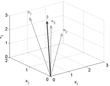
Figure 1 shows the geometric representation of the four vectors in a three-dimensional Euclidian

space. Observe that vector  is closer to 3 than to the other vectors although  actually stays in the

plane spanned by ₁ and ₂. This is because vector ₃ can be decomposed as

3 0.5 1 0.5 2 3

 _  _  _  ₍₁₅₎

where ₃=[0.1 -0.2 0.1]T. Vector 3is actually composed of two components: the component which

lies in the plane spanned by 1 and 2 and a small component 3

 _{which is perpendicular to the plane}

and has no contribution to the explanation of the dependent vector . Hence vector 3 possesses

both the information of 1 and the information of 2.

Fig 1 The geometric relations of the vectors in (13)

The standard OFR process is to find a sequence of nesting subspaces S1S2 Ssstep by step.

10

regression matrix is optimal at each step. Here optimal means the orthogonal projection of y on Sk is

maximal. In order to decouple the contribution of each term to the total projection, the k-th term is

orthogonalised to the (k-1) terms selected in the earlier steps so that the projection can be calculated

stepwise. The k orthogonal terms form a k-dimensional orthogonal basis of space Sk. Denote the sum

of the ERR values at the k-th step as

1 k

k i

i

SERR ERR







normalised measurement to the projection. Mao and Billings (1997) argued that when using the

orthogonal algorithm to detect the model structure, previously selected terms can influence the

selection of later terms. Therefore the detection of a minimal model structure can be considered as a

search for the optimal orthogonalisation path which is defined as the order in which candidate terms

are orthogonalised into the regression equation.

In order to analyse the effects of orthogonalisation paths, all the possible orthogonalisation paths are

listed in Table 1. For this example, there are a total number of 6 different orthogonalisation paths in

which three terms can be orthogonalised into a model.

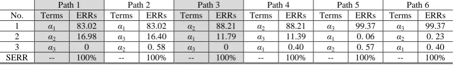
Table 1 ERRs along the six different orthogonalisation paths for eq. (14)

Path 1 Path 2 Path 3 Path 4 Path 5 Path 6 No. Terms ERRs Terms ERRs Terms ERRs Terms ERRs Terms ERRs Terms ERRs

1 1 83.02 1 83.02 2 88.21 2 88.21 3 99.37 3 99.37

2 2 16.98 3 16.40 1 11.79 3 11.39 1 0. 06 2 0. 23

3 3 0 2 0. 58 3 0 1 0.40 2 0. 57 1 0. 40

SERR -- 100% -- 100% -- 100% -- 100% -- 100% -- 100%

Along the six different paths, the orthogonalised terms form six different orthogonal bases which are

shown in Fig 2. Projecting  on each of the orthogonal bases, the ERR values are given in Table 1.

11

An optimal model means the smallest model which includes all the correct terms. In the language of

the ERR framework, an optimal model includes the smallest number of terms but produces the largest

sum of ERR values. In this example, the optimal model is composed of the two correct terms 1 and

2

 . The classic OFR algorithm searches for a solution along a path where the sum of the ERR’s

increases at the fastest speed. In this example, although vector  is on the plane spanned by 1 and

2

 , the first term that will be selected by the OFR algorithm is 3 because 3 is the term which is

mostly close to  and gives the largest projection, see Fig 1. Therefore, the OFR will orthogonalise

the regressors along path 6 in Table 1, ₃₂₁. However following path 6 the obtained model

is not optimal. When a specific tolerance is taken, for example, =0.50%, a correct term will be

missed along path 4, and 6 while a redundant term will be selected along path 2 and 5. However along

both paths 123 and 213, the search process produces an optimal model which

consists of two correct terms for any tolerance less than 10%. This means that along a correct

orthogonalisation path the algorithm will be much more robust, to yield optimal results, and the cutoff

is much more obvious and easier to select.

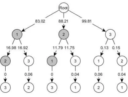
In a forward regression process, since the terms are selected one by one into a model, all the

orthogonal paths comprise a solution tree. At the first step, there are  options 1, , which

represent the  direct child nodes of the root node. These direct child nodes divide the whole tree into

 branches and each of the branches is also of a tree structure. There are ( 1) options at the second

step and (2) options at the third step, and so on. There are a total number of ! different

orthogonalisation paths. A forward regression method starts from the common root node and selects

terms one by one from an upper layer to a lower layer. The ERR values assign a weight for each

branch of the tree. Each path from the root node to a leaf node represents a complete

orthogonalization path along which a corresponding model can be obtained. For the example under

12

Fig 3 Solution tree of a forward regression algorithm for eq. (14)

For a globally optimal solution, we would need to search on the whole tree and evaluate all the

solutions on the different branches. Observe that there are many opportunities to find a correct

solution by exhausting all the paths on the solution tree. For a correct model which consists of m

terms there are a total number of m! different perturbations, where ( )! represents the factorial

operation, and each represents a correct solution on different branches of the solution tree. There are a

total number of m! optimal solutions on the tree. These optimal solutions can only happen on the

paths which start from a correct term. Hence only the sub-trees which start from a correct term need to

be considered when searching for an optimal solution. In the above example, there are two optimal

orthogonalisation paths and only the branches starting from ₁ and ₂ may include the optimal

solution.

A classic OFR algorithm can occasionally search along a wrong orthogonalisation path by picking a

wrong term in the first steps. As a result, the search process will be along a wrong path and produce a

sub-optimal model. From the root node, a searching process can be forced onto a certain sub-tree by

fixing the first term before the searching process proceeds. Therefore an intuitive idea is to use the

OFR algorithm to search on each of the sub-trees. A sub-optimal model is obtained on each sub-tree.

Compare these obtained models and choose the best one as the final result. The optimal model will be

in these sub-optimal models. Remember that there are a total number of m! opportunities to find a

13

from a wrong term will never give an optimal model. Therefore, only the sub-trees starting from a

correct term need to be considered. However, it is unknown which term is a correct term.

Nevertheless a suboptimal model can always be a good starting point for the search for an optimal

solution. It is reasonable to assume that a suboptimal model consists of a majority of correct terms and

a few incorrect terms. Therefore an iterative learning algorithm can be proposed to find an efficient

and intuitive solution to this problem. The new iterative OFR algorithm consists of the following steps.

i). Preset a tolerance  and apply the standard OFR algorithm on the whole term dictionary

to produce a suboptimal term set





1 2 s

s  s s s ;

ii). Select a small number  as an amendment to the tolerance in the first step (see Remarks 2

for the choice of );

iii). Select one of the terms _j( ₁, ₂, ,

s

js s s ) in s as a preselected first term and search the

other terms on the term set \

 

1



iv). Repeat iii) for all the i’s in s and obtain s suboptimal models;

v). Compare the obtained s suboptimal models and choose the best one as the final model op .

NARMAX models which typically include highly correlated unknown noise terms can be identified

by following the iterative procedure below. Because the noise terms are not known a priori the model

prediction errors (residuals) will be used to approximate the noise terms.

i). Assume the noise terms are zero and identify the model which does not included the noise

terms using the iOFR algorithm.

ii). Produce the prediction errors using the best model obtained in step i).

iii). Use the residuals as the noise terms and construction the new term dictionary in which the

delayed noise terms are included.

iv). Identify the full NARMAX model from the dictionary obtained in step iii) using the iOFR

14

v). Repeat steps ii) - iv) until a satisfying model obtained. At each time the residuals are

calculated based on the new identified model. Validate the model.

Remarks:

1) The searching process can be further iterated by selecting op as the suboptimal solution s in

step i) and repeating steps ii) ~ v) for a better result. This time only terms in the set





: | ,

s op   op and op need to be considered. However further iterations are often not

needed. An optimal solution may be found in the first iteration because the OFR algorithm itself is

powerful in searching for an optimal solution but more steps may be needed in some cases.

2) The amendment  of the tolerance often takes a small non-negative number. A tolerance 

means the sum of ERR’s of the selected terms in a model is no less than (1). Hence the larger a

tolerance  is, the less terms will be selected in the obtained model. A positive  means ( )

is a stricter tolerance and the iterative process will eliminate some of the redundant terms to produce a

smaller model. On the contrary, a negative  means ( ) is a looser tolerance and the iterative

process will select more terms into the model and produce a more accurate description. An increase of

the tolerance by  can significantly tighten the search process to produce a smaller model. At the

same time a small  will not expel the correct terms. For example, a good choice of the absolute

value of  can be the ERR value of the least significant term in s , that is,

 





min ERR _i | _{i s}



   . This follows because after all the correct terms have been selected, the

remaining terms are considered as redundant terms and the corresponding contributions will be much

smaller than the one with the smallest contribution in the suboptimal model. Since the new iOFR

searches for solutions on several sub-trees in parallel and chooses the best model as the result it can be

expected that the model which is obtained in the iterative process will be no worse than the

sub-optimal model in the first step when the tolerance is keeps kept unchanginged. Hence another often

15

the model, the sum of ERR’s will reach (1) more quickly and a more parsimonious model is

obtained.

3) In the classic OFR algorithm, the selection of the tolerance  is crucial for the identification of the

model. Additionally, the selection of the tolerance is often problem-dependent. For example, the

tolerance may depend on the noise level in the measurement of the input and output. A tight tolerance

may expel some correct terms while a loose tolerance may cause overfitting of the data. In the classic

OFR algorithm, a wrong term is selected in to a model because the wrong term may include the

information of more than one correct term and this becomes more significant at the first steps of the

forward selection process. Selecting the wrong term into the model at an early stage will make the

correct terms much less significant and the correct terms will be selected into the model later to

compensate for the information which has been missed. When the remaining unexplained information

is small and is comparable to the effects of noise, a slight change in the tolerance may lead to a

different model the tolerance will become very sensitive. Hence accurate determination of the

tolerance under which no correct terms will be missed can be difficult. This can be avoided by using

the new iOFR algorithm. When any of these correct terms has been forced to be the first term, the

contribution of the wrong term becomes much less significant because part of the information has

been explained by the pre-determined correct terms which has been selected in the previous steps. As

a result, there is a much lesser possibility that the wrong term will be selected at the following steps.

Along a correct orthogonalisation path all the correct terms will be significant and the OFR algorithm

will be more robust to the value of the tolerance. This has been observed in the previous example

where any tolerance which is not greater than 10% will lead to the correct model. Hence, the setting

of the tolerance  can be relatively flexible in the new iOFR algorithm. This feature of the iOFR can

be very useful in the identification of real systems.

4) Unlike a coarse-to-fine algorithm which starts from a sub-optimal model and purely eliminates

redundant terms, In the iterative stepsOFR algorithm, the search process is not operated search terms

16

the pre-determined term i. This enables the iOFR algorithm to select find the correct terms which

have been missed in the by the sub-optimal model which is obtained at in the first stage into the final

model toand obtain a better solution. In other words, the new iOFR algorithm does not need the

suboptimal model obtained at the first step to be a sufficient model. This will be observed in the

example in Section 4.2.

The new iOFR algorithm may occasionally give a suboptimal solution since the algorithm only tries

different routes at the first step and the remaining term selection could still follow a suboptimal trace.

However this will happen with a very low probability. Firstly, the new iOFR searches the optimal

model in parallel along several different paths on the whole solution tree. According to the previous

discussion, there are a total number of m! opportunities to find the optimal model and hence the

probability at which the iOFR can find the optimal solution will increase significantly. The

improvement in the possibility to find the optimal solution will be discussed below. Secondly, along

the different search paths the corresponding orthogonal basis will be quite different and the ERR’s

assigned to each term will change accordingly. The significant terms will then be selected into the

term in a different order. This has been observed in the example given in Fig 2. To some extent, this

process works like the heating process in a simulated annealing algorithm where the metal atoms in

the material will be rearranged to build a better crystal structure in the cooling process. Finally,

according to the previous discussion, the significance of a wrong term which may be selected in the

first steps because it contains information from the correct terms will be greatly reduced when any of

the correct terms has been firstly selected. In the selection of the remaining terms, the wrong term will

be less likely to be selected although the search is still along the speediest increasing path of the sum

of ERR values. Based on the above discussion, these are probably the best solutions available because

the alterative full optimal search (Mao and Billings 1997) involves a huge computational overload

that is just not feasible when studying real data sets where it is often necessary to try lags over the

range 1-30 in the initial search. Noise model terms and MIMO (multi-input-multi-output) systems just

17

We should ask what the probability is that the new iOFR algorithm will produce an optimal solution.

Assume 1 terms in a s-s terms of the suboptimal model s which were was obtained at the first

stage and are correct; the OFR algorithm can find an optimal solution with a probability of p along

each path starting with a correct term. The iOFR algorithm will search the optimal solution along s

parallel paths. The probability that the iOFR will find the optimal solution on at least one path will be

1

1 (1 p) , which equals to one minus the probability that the iOFR fails to find the optimal solution

on all the paths, seeing that the search along the ( s ₁) paths which start with a wrong term will

have no contribution for to the probability. The probability will be much higher than the probability of

the single path search when ₁ is large enough. For example, consider a suboptimal model which

consists of s20 terms in which  1 10 terms are correct terms. The iOFR algorithm searches for

the optimal solution along 10 parallel paths at a probability of 50% on each path. It is easy to calculate

that the probability that the iOFR algorithm will find the optimal solution is _{(1 0.5 )} 10 _{99.9% which}

is much higher than the 50% succession probability of the single path search algorithm. In fact, the

probability for the classic OFR to successfully find the optimal solution is much better than 50%.

Even the classical OFR can produce an optimal solution in most cases except in some special

situations.

The new iOFR algorithm is also computationally efficient. As discussed in the paper (Mao and

Billings 1997), there are a total number of ! orthogonalization orthogonalisation paths for a  term

dictionary, where ( )! represents the factorial operation. Searching for an optimal solution by

exhausting all these paths is computationally just not practical. Applying the genetic algorithm

assistant MMSD (Minimal Model Structure Detection) algorithm the search space can be reduced to a

much more practical number which can still be a large number. Comparatively, in the new iOFR

algorithm, the number of searching paths depends on the number of terms in the sub-optimal model

obtained at the first stage which is much less than the size of the full dictionary, without mentioning

the number of all the combinations. Consider the example in the Mao and Billings paper where 20

18

MMSD algorithm searches along_{2 10} 3_{paths. Using the new iOFR algorithm, no more than 20 best}

searching paths which start from the terms in a suboptimal model need to be evaluated. Therefore it

can be concluded that the new iOFR algorithm is very efficient. A discussion of the computational

complexity of the classic OFR algorithm has been given in the references.

The performance of the new iOFR algorithm can be improved by appropriately increasing the number

of parallel searches. For example, a smaller tolerance in the first stage will lead to a sub-optimal

model with more terms and the global search at the second stage will be carried out on more parallel

sub-trees. The iOFR algorithm can also be improved by increasing the number of the pre-selected

terms where a subset instead of a term in _s is determined. The more correct terms are

pre-determined, the less possibly the wrong term will be selected into the final model. However, both

improvements lead to an increase in computational complexity.

An alternative OFR algorithm has been proposed by Piroddi and Spinelli (2003) based on minimising

the model predicted or simulated output rather than the one step ahead predictions. This is very

similar to the algorithms by Billings and Mao (1998). The simulated output based algorithm has been

shown to be effective where the data is grossly oversampled and where the input is badly designed

and not persistently exciting. However, these solutions are hugely computationally expensive so that

they cannot be realistically applied to complex models where searches over many lags, MIMO models,

and noise are involved all of which are typical when dealing with real data sets rather than very

simple simulated examples. The new iOFR offers a much simpler solution.

4. Test examples

Several examples will beare used to illustrate the new iOFR algorithm. While the literature is full of

examples where the classical OFR algorithm works extremely well, each example below has been

deliberately chosen from the small number of past results where the standard OFR has been shown to

19

examples where the data is sampled correctly and the input is persistently exciting the algorithm

works perfectly every time.

4.1. A linear example

This linear example will beis used to show that the OFR algorithm can sometimes give a suboptimal

model which includes redundant terms. But by applying an iterative process, the OFR algorithm is

greatly improved and is able to produce an optimal solution. This example was taken from (Wei and

Billings 2008).

Consider the system

 







 





  

y k   y k  y k u k  u k e k (16)

where y(k), u(k), and e(k) represent the output, input and noise of the system. The input is uniformly

distributed white noise u(k) ~ U(-1,1). The noise is normally distributed white noise e(k) ~ N(0,0.12).

A total number of 1000 input and output data are measured for the system identification. Define a

candidate term dictionary which is composed of the delayed input and output terms ={1),

y(k-2), y(k-3), y(k-4), y(k-5), u(k-1), u(k-y(k-2), u(k-3), u(k-4), u(k-5)}. Applying the classic OFR algorithm,

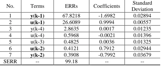
the identified model is shown in Table 1. A total number of seven terms have been selected into the

model which includes all the correct terms. However three redundant terms have also been selected.

Table 2 Results given by the standard OFR algorithm for system (16)

No. Terms ERRs Coefficients Standard Deviation

1 y(k-1) 67.8218 -1.6982 0.02894

2 u(k-1) 26.6089 0.9994 0.00557

3 y(k-4) 2.8635 0.0017 0.01235 4 u(k-4) 0.5968 -0.0021 0.01396 5 u(k-3) 0.4825 0.0036 0.01325

6 u(k-2) 0.4121 0.7912 0.02944

7 y(k-2) 0.3908 -0.7992 0.03679

SERR -- 99.18 -- --

In this example the classic OFR algorithm gives an incorrect model because of under-sampling.

20

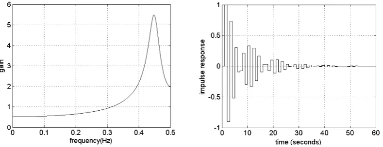
frequency. The frequency response function and impulse response of system (16) (see Figure 4) show

that the natural frequency of the system is around 0.45 Hz. The sampling frequency in this example is

1 Hz which is only about 2.2 times of the natural frequency. The severe under-damping in the system

exasperates this problem. The impulse response shows that the system needs a long time to settle

down and oscillates with a period about 2.2s. This means the response of the system will repeat every

2.2s (about 2 sampling intervals). Since the output is a convolution of the input with the impulse

response function, y(k) may be of a similar pattern with y(k-2). This explains why y(k-4) may appear

in the final model because the term looks like y(k-2) for this sampling and data case. The effect of

sampling time on nonlinear system identification has been studied by Billings and Aguirre (1995), and

Billings (2013).

Figure 4 Frequency response function and impulse response of system (16)

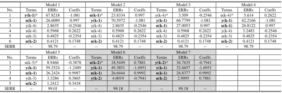
Taking each term in Table 2 as the first term and applying an OFR algorithm where =0.3908 %

which is the least value of the ERR’s in Table 2, yields the results of the iOFR process given in Table

3. Seven different models were obtained. Models 6 and 7 have the simplest structure where only four

terms are used to produce the best SERR. Actually both models consist of four correct terms. Models

1, 2, 3, 4, and 5 missed the correct term y(k-2) under the amended tolerance ( ) and produce a

relatively smaller SERR. Therefore model 6 and model 7 are selected as the final results of the iOFR

21

redundant terms in Table 2 have been successfully eliminated in the iterative process. The iOFR

algorithm which starts from the results of a standard OFR process gave gives the optimal model.

Table 3 Results produced by iOFR algorithm for system (16)

Model 1 Model 2 Model 3 Model 4

No. Terms ERRs Coeffs Terms ERRs Coeffs Terms ERRs Coeffs Terms ERRs Coeffs

1 y(k-1)* 67.8218 -1.081 u(k-1)* 23.8334 0.997 y(k-4)* 3.509 -0.2546 u(k-4)* 5.614 0.2622

2 u(k-1) 26.6089 0.997 y(k-1) 70.5972 -1.081 y(k-1) 66.7799 -1.081 y(k-1) 62.2166 -1.081

3 y(k-4) 2.8635 -0.2546 y(k-4) 2.8635 -0.2546 u(k-1) 27.0053 0.997 u(k-1) 26.8122 0.997 4 u(k-4) 0.5968 0.2622 u(k-4) 0.5968 0.2622 u(k-4) 0.5968 0.2622 y(k-4) 3.2483 -0.2546 5 u(k-3) 0.4825 -0.2354 u(k-3) 0.4825 -0.2354 u(k-3) 0.4825 -0.2354 u(k-3) 0.4825 -0.2354

6 u(k-2) 0.4121 0.1748 u(k-2) 0.4121 0.1748 u(k-2) 0.4121 0.1748 u(k-2) 0.4121 0.1748

SERR -- 98.79 -- -- 98.79 -- -- 98.79 -- -- 98.79 Model 5 Model 6 Model 7

No. Terms ERRs Coeffs Terms ERRs Coeffs Terms ERRs Coeffs 1 u(k-3)* 8.9466 -0.3878 u(k-2)* 18.5449 0.7881 y(k-2)* 36.7635 -0.7941

2 y(k-1) 59.2524 -1.2489 y(k-1) 49.3851 -1.6951 y(k-1) 32.6657 -1.6951

3 u(k-1) 26.2424 0.9987 u(k-1) 26.6444 0.9992 u(k-1) 26.8377 0.9992

4 y(k-3) 3.3286 0.3865 y(k-2) 4.6019 -0.7941 u(k-2) 2.9095 0.7881

5 u(k-2) 1.2412 0.3418

SERR -- 99.01 -- -- 99.18 -- -- 99.18 -- * means the term is determined first.

4.2. A nonlinear example

This example is taken from (Mao and Billings 1997). System (17) has been widely used as a

benchmark example for the study of variations of OFR algorithms and for comparisons of OFR with

other algorithms (Baldacchino et al.). In this example, it will be shown that the iOFR can produce an

optimum solution even when some correct terms are not selected in the first OFR step.

Consider the nonlinear system

 







 













 

  

3 2

2

0.2 1 0.7 1 1 0.6 2 0.5 2

0.7 2 2

y k y k y k u k u k y k

y k u k e k

        

    (17)

The system is excited with a uniformly distributed white noise u(k) ~ U(-1,1) and the output y(k) is

disturbed by a normally distributed white noise e(k) ~ N(0,0.12). A total number of 1000 input and

output data were used for the system identification.

Up to third order polynomials of the delayed inputs and outputs {y(k-1), y(k-2), y(k-3), y(k-4), u(k-1),

u(k-2), u(k-3)} were used to model the nonlinear system. A total number of 120 terms were included

in the term dictionary . Applying the OFR algorithm yields a five term model which is shown in

Table 4. Notice that the model in Table 4 includes an redundant term y(k-4)u2(k-2) but misses a

22

Table 4 Results produced by the standard OFR algorithm for system (17)

No. Terms ERRs Coefficients Standard Deviation 1 y(k-4)u2(k-2) 36.2732 0.2922 0.02602

2 y(k-1)u(k-1) 13.7147 0.6544 0.01528

3 u2(k-2) 11.3488 0.5134 0.009331

4 y(k-2) 26.8516 -0.6743 0.01165

5 y3(k-1) 3.3248 0.1949 0.009847

SERR -- 91.513 -- --

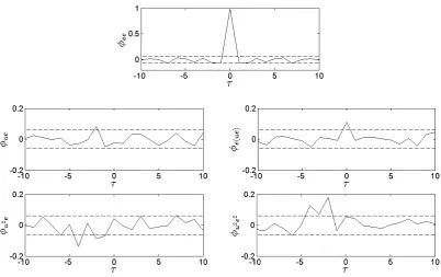
The nonlinear cross correlation model validation tests (Billings and Voon 1986; Billings and Zhu

1994) clearly show that the model is unacceptable as a sufficient model of system (17). Figure 5

shows that the cross correlation tests fail with two of the five cross correlations significantly outside

the 95% confidence intervals. Notice that this model has been obtained by deliberately abusing the

classic OFR algorithm to test the robustness of the new iOFR algorithm. In the application of the OFR

algorithm, a model validation is always adopted conducted to aid the determination of the model size.

An obtained model should be sufficient enough to pass all the model validations. For this example, an

acceptable model can be obtained by increasing the number of terms until the model validations are is

satisfied.

23

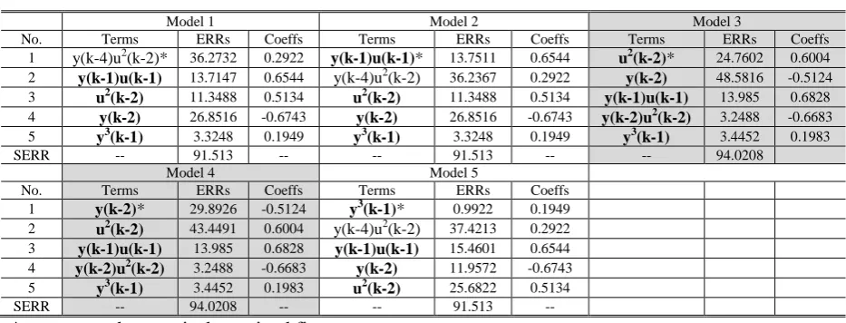
Take the incorrect model in Table 4 as the starting point and apply the iOFR algorithm. Use each term

in the previous model as the first term and employ the OFR algorithm to select the remaining terms

until SERR satisfies a tolerance where =0. The new iOFR produced five different models. The

results are shown in Table 5. All the five models have the same number of terms. However models 3

and 4 give a better SERR than the other three models. Compared with system (17), both models 3 and

model 4 are composed of the correct terms and give an accurate representation of the original system.

It is worth emphasising that the missed term y(k-2)u2(k-2) in Table 3 has now been correctly selected

into the final model by the iOFR algorithm.

Table 5 Results produced by iOFR algorithm for system (17)

Model 1 Model 2 Model 3

No. Terms ERRs Coeffs Terms ERRs Coeffs Terms ERRs Coeffs

1 y(k-4)u2(k-2)* 36.2732 0.2922 y(k-1)u(k-1)* 13.7511 0.6544 u2(k-2)* 24.7602 0.6004 2 y(k-1)u(k-1) 13.7147 0.6544 y(k-4)u2(k-2) 36.2367 0.2922 y(k-2) 48.5816 -0.5124

3 u2(k-2) 11.3488 0.5134 u2(k-2) 11.3488 0.5134 y(k-1)u(k-1) 13.985 0.6828

4 y(k-2) 26.8516 -0.6743 y(k-2) 26.8516 -0.6743 y(k-2)u2(k-2) 3.2488 -0.6683

5 y3(k-1) 3.3248 0.1949 y3(k-1) 3.3248 0.1949 y3(k-1) 3.4452 0.1983

SERR -- 91.513 -- -- 91.513 -- -- 94.0208

Model 4 Model 5

No. Terms ERRs Coeffs Terms ERRs Coeffs

1 y(k-2)* 29.8926 -0.5124 y3(k-1)* 0.9922 0.1949

2 u2(k-2) 43.4491 0.6004 y(k-4)u2(k-2) 37.4213 0.2922 3 y(k-1)u(k-1) 13.985 0.6828 y(k-1)u(k-1) 15.4601 0.6544 4 y(k-2)u2(k-2) 3.2488 -0.6683 y(k-2) 11.9572 -0.6743

5 y3_{(k-1) 3.4452 0.1983 u}2_{(k-2) 25.6822 0.5134}

SERR -- 94.0208 -- -- 91.513 --

* represents the term is determined first.

In both examples, the new iOFR algorithm produced optimal models which include all the correct

terms and are of the simplest structure in a very efficient computational process. The iOFR algorithm

worked well even when the first OFR step did not give a correct model as in the second example.

Moreover, in both examples, the iOFR algorithm found optimal solutions on more than one searching

path. This indicates that the new algorithm is significantly robust because the iOFR can still produce

an optimal solution even when the algorithm fails on one of the parallel search paths.

4.3. A nonlinear example with noise modelling

This example is taken from and uses the same settings in the Piroddi and Spinelli’s paper with the

same parameter settings (Piroddi and Spinelli 2003). This example will be used to show that the iOFR

24

This example also illustrates the application of iOFR in identification of NARMAX models including

delayed noise terms.

The system is given as follows

 













 

3

1

1 0.5 2 0.25 ( 1) ( 2) 0.3 1

1

( ) ( )

1 0.8

w k u k u k u k u k u k

y k w k e k

z                _  (18)

where u represents the input signal and y represents the observation of the output w. Both the input

u(k) and the noise e(k) are Gaussian distributed white noise. It can be shown that the classic OFR

algorithm can correctly select all the terms and produce an accurate model when the system is

persistently excited. However, Piroddi and Spinelli argued that the classic OFR algorithm may

incorrectly select autoregressive terms when the input signal is less not rich enough in frequency

components. Piroddi and Spinelli recommended an input which is generated by an AR process with

two real poles between 0.75 and 0.9. Repeating Piroddi and Spinelli’s simulation using an input signal

which was generated by the following AR process.

1 2

0.3

( ) ( )

1 1.6 0.64

u k v k

z z



  (19)

where v(k) is Gaussian noise v(k) ~ N(0,1). The AR process has a repeat pole at 0.8 and the coefficient

0.3 is chosen to guarantee the input signal is at a reasonable level. Here the noise signal e(k) is a

Gaussian distributed noise with a variance 0.02, that is, e(k) ~ N(0,0.02). The results produced by the

classic OFR algorithm are given in Table 6.

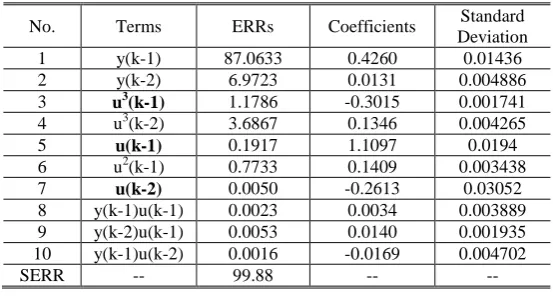
Table 6 Results produced by the classic OFR algorithm for example 3

No. Terms ERRs Coefficients Standard Deviation 1 y(k-1) 87.0633 0.4260 0.01436 2 y(k-2) 6.9723 0.0131 0.004886

3 u3(k-1) 1.1786 -0.3015 0.001741

4 u3(k-2) 3.6867 0.1346 0.004265

5 u(k-1) 0.1917 1.1097 0.0194

6 u2(k-1) 0.7733 0.1409 0.003438

7 u(k-2) 0.0050 -0.2613 0.03052

8 y(k-1)u(k-1) 0.0023 0.0034 0.003889 9 y(k-2)u(k-1) 0.0053 0.0140 0.001935 10 y(k-1)u(k-2) 0.0016 -0.0169 0.004702 SERR -- 99.88 -- --

Observe that several incorrect autoregressive terms have been selected overwhelming the correct

terms while a correct term u(k-1)u(k-2) was is missed. The new iOFR algorithm was employed to

solve the problem. Each term in the model in Table 6 was selected as the pre-determined term and the

25

number of 10 models were obtained. Three in the ten models give the same model which is the best

model obtained under the given tolerance of 0.2%.

Table 7 Model identified using the iOFR algorithm for example 3

No. Terms ERRs Coefficients Standard Deviation

1 u3(k-1) 79.8101 -0.3002 0.000578

2 u(k-1) 14.4655 0.9686 0.01938

3 u (k-1)u(k-2) 5.3722 0.2485 0.001905

4 u(k-2) 0.1596 0.5413 0.01864

5 constant 0.0050 0.0477 0.009254 SERR -- 99.81 -- --

Next we generated the residuals ( )k y k( )y kˆ( ), where y kˆ( ) is the one-step-ahead prediction of the

model in Table 7. Use We then used the residuals to replace the noise terms. The new dictionary is

composed of all the up to third order monomials of variables {u k( 1), u k( 2), y k( 1), y k( 2),

(k 1)

  ,(k2),(k3)}. The new iOFR is was then used to identify the full NARMAX models

form the constructed dictionary under the tolerance level 0.2%. This time three of seven search paths

gave the optimal solution which is shown in Table 8. All the terms in system (18) were successfully

detected and the associated coefficients are close to the real values in the first time iteration for the

noise model.

Table 8 Full model identified using the iOFR algorithm for example 3

No. Terms ERRs Coefficients Standard Deviation

1 u3(k-1) 79.8129 -0.2995 0.000349

2 u(k-1) 14.4635 0.9647 0.012

3 u (k-1)u(k-2) 5.3719 0.2543 0.000933

4 u(k-2) 0.1591 0.5395 0.01156

5 (k - 1) 0.1174 -0.7922 0.01968 SERR -- 99.92 -- --

5. Conclusions

Several algorithms have been proposed to enhance the OFR algorithm by introducing modified or add

on algorithms, but the new iterative orthogonal forward regression algorithm improves OFR under a

26

algorithm which is also highly computationally efficient. The new iOFR improves the classic OFR in

two ways: it eliminates the redundant terms in a suboptimal model to produce a more parsimonious

model, and selects the correct terms to obtain an accurate system description. Because the new iOFR

searches for the solution over the whole solution tree iOFR is capable of producing an optimal

solution using simple search procedures and can be applied to estimate highly complex system models

within a very efficient and intuitive framework.

Acknowledgements

The authors gratefully acknowledge support from the UK Engineering and Physical Sciences

Research Council (EPSRC) and the European Research Council (ERC).

References

Baldacchino, T., Anderson, S. R., and Kadirkamanathan, V. "Computational system identification for Bayesian NARMAX modelling." Automatica, 49(9), 2641-2651.

Billings, S. A. (2013). Nonlinear system identification : NARMAX methods in the time, frequency, and spatio-temporal domains, John Wiley & Sons Ltd, Hoboken, New Jersey.

Billings, S. A., and Aguirre, L. A. (1995). "Effects of the sampling time on the dynamics and identification of nonlinear models." International Journal of Bifurcation and Chaos, 5(6), 1541-1556.

Billings, S. A., and Chen, S. (1989). "Extended model set, global data and threshold-model identification of severely non-linear systems." International Journal of Control, 50(5), 1897-1923.

Billings, S. A., Chen, S., and Korenberg, M. J. (1989). "Identification of MIMO non-linear systems using a forward-regression orthogonal estimator." International Journal of Control, 49(6), 2157-2189.

Billings, S. A., Korenberg, M. J., and Chen, S. (1988). "Identification of non-linear output-affine systems using an orthogonal least-squares algorithm." International Journal of Systems Science, 19(8), 1559-1568.

Billings, S. A., and Mao, K. Z. (1998). "Model identification and assessment based on model predicted output."

Billings, S. A., and Voon, W. S. F. (1986). "Correlation based model validity tests for nonliear models." International Journal of Control, 44(1), 235-244.

Billings, S. A., and Wei, H.-L. (2007). "Sparse Model Identification Using a Forward Orthogonal Regression Algorithm Aided by Mutual Information." Neural Networks, IEEE Transactions on, 18(1), 306-310.

Billings, S. A., and Zhu, Q. M. (1994). "Nonlinear model validation using correlation tests." International Journal of Control, 60(6), 1107-1120.

27

Leontaritis, I. J., and Billings, S. A. (1985). "Input-output parametric models for non-linear systems Part I: deterministic non-linear systems." International Journal of Control, 41(2), 303-328. Li, K., Peng, J.-X., and Bai, E.-W. (2006). "A two-stage algorithm for identification of nonlinear

dynamic systems." Automatica, 42(7), 1189-1197.

Mallat, S. G., and Zhang, Z. (1993). "Matching pursuits with time-frequency dictionaries." Signal Processing, IEEE Transactions on, 41(12), 3397-3415.

Mao, K. Z., and Billings, S. A. (1997). "Algorithms for minimal model structure detection in nonlinear dynamic system identification." International Journal of Control, 68(2), 311-330. Pati, Y. C., Rezaiifar, R., and Krishnaprasad, P. S. "Orthogonal matching pursuit: recursive function

approximation with applications to wavelet decomposition." Signals, Systems and Computers, 1993. 1993 Conference Record of The Twenty-Seventh Asilomar Conference on, 40-44 vol.1. Piroddi, L., and Spinelli, W. (2003). "An identification algorithm for polynomial NARX models

based on simulation error minimization." International Journal of Control, 76(17), 1767-1781. Sherstinsky, A., and Picard, R. W. (1996). "On the efficiency of the orthogonal least squares training

method for radial basis function networks." Trans. Neur. Netw., 7(1), 195-200.

Shouche, M., Genceli, H., Premkiran, V., and Nikolaou, M. (1998). "Simultaneous Constrained Model Predictive Control and Identification of DARX Processes." Automatica, 34(12), 1521-1530.