Unspanned macroeconomic factors in the yield curve

This is a repository copy of

Unspanned macroeconomic factors in the yield curve

.

White Rose Research Online URL for this paper:

http://eprints.whiterose.ac.uk/90596/

Version: Accepted Version

Article:

Coroneo, Laura orcid.org/0000-0001-5740-9315, Giannone, Domenico and Modugno,

Michele (2015) Unspanned macroeconomic factors in the yield curve. Journal of Business

and Economic Statistics. ISSN 0735-0015

https://doi.org/10.1080/07350015.2015.1052456

Reuse

Unspanned macroeconomic factors in the yield curve

Online Appendix

Laura Coroneo University of York

Domenico Giannone

Federal Reserve Bank of New York CEPR, ECARES and LUISS

Michele Modugno

Board of Governors of the Federal Reserve System

April 3, 2015

D

Unrestricted vs block-diagonal macro-yields model

In this Appendix we report results for two alternative macro-yields models that use different

as-sumptions about the matrix of factor loadings Γ in Equation 4 in the main text. The first model

that we consider is an unrestricted macro-yields model, which does not impose the zero restrictions

on the factor loadings of yields on macro factors, i.e. Γyx is allowed to be different from zero.

This model allows the macro factors F_tx to directly affect the cross-section of yields. The second model imposes block-diagonality of the matrix of factor loadings Γ, i.e. Γyx = 0 and Γxy = 0.

This implies that the yield curve factors and the macro factors are treated separately, as in M¨onch

(2012). Notice that when estimating the block-diagonal macro-yields model, we omit the federal

funds rate from the macro variables used to estimate the model, as in M¨onch (2012). The reason

is that we cannot reliably impose a zero restriction on the factor loadings of the federal funds rate

on the yield curve factors.

Results in Tables 1–4, show that the in-sample and out-of-sample performances of the

factors in Tables 1, 2, and 5 in the main text. This provides evidence that the zero restrictions on

the factor loadings are satisfied by the data, implying that the macro factorsFx

t are unspanned by

the cross-section of yields.

On the contrary, imposing a block-diagonal structure on the matrix of factor loadings has

substantial implications for the the identification of the factors. Table 1 shows that the information

criterion selects the model with six factors, i.e. three yield curve factors and three macro factors.

This indicates that this model is less parsimonious than our macro-yields model. In addition, as

shown in Table 2, the macro factors in the block-diagonal macro-yield model are highly correlated

with the yield curve factors and are, thus, spanned by the cross-section of yields. This happens

because the macro variables have a factor in common with the yields which the block-diagonal

model treats as an additional macro factor. Table 2 also shows that the correlation of the first

macro factor of the block-diagonal macro-yields model with the industrial production index is

weaker than in our model. More importantly, the second and third macro factors do not have a

clear-cut interpretation.

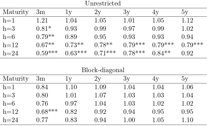
The fit of the block-diagonal macro-yields model is comparable to the fit of our macro-yields,

as shown in Table 3. However, in spite of the fact that our model has less factors than the

block-diagonal model, the forecasting performances of the macro-yields model are not worse than the

ones obtained from the block-diagonal macro-yields model, on the contrary there is some evidence

of improved accuracy. This suggests that in our model the eventual loss of information is more

than compensated by the gains in the reduction of estimation uncertainty implied by the more

parsimonious structure. In summary, this confirms that the extra macro-factor in the block diagonal

Table 1: Model selection

Unrestricted Block-diagonal

Number of factors IC* V IC* V

3 0.02 0.44 1.17 1.36

4 -0.02 0.31 1.30 1.16 5 -0.11 0.22 1.50 1.05

6 0.01 0.18 0.89 0.43

7 0.25 0.17 1.06 0.38

8 0.43 0.16 1.42 0.41

This table reports the information criterion IC*, as shown in equation (7) and in equation (8), and the sum of the vari-ance of the idiosyncratic components (divided by NT), V , when different numbers of factors are estimated. The first two columns refer to the unrestricted macro-yields model. The last two columns refer to the block-diagonal macro-yields model.

Table 2: Factor identification

Unrestricted

L S C M1 M2

NS L 0.98 0.00 0.32 -0.08 0.01 NS S 0.03 0.97 0.28 0.11 0.08 NS C 0.25 0.37 0.86 0.12 0.06 IP -0.08 0.03 0.16 0.91 -0.09 R 0.47 0.05 0.10 0.20 -0.76

Block-diagonal

L S C M1 M2 M3

NS L 0.99 -0.03 0.21 -0.07 0.46 0.57 NS S -0.03 0.99 0.38 0.51 0.44 -0.38 NS C 0.18 0.36 0.98 0.36 0.22 0.13 IP -0.10 0.04 0.20 0.69 -0.49 0.20 R 0.44 0.08 0.15 -0.05 -0.35 0.20

Table 3: In sample performance

Unrestricted Model

L S C M1 M2

Average Hourly Earnings:Total Private 0.07 0.29 0.33 0.33 0.67 Consumer Price Index: All Items 0.19 0.48 0.48 0.50 0.86 Real Disposable Personal Income 0.00 0.02 0.03 0.34 0.36 Effective Federal Funds Rate 0.54 0.93 0.96 0.96 0.97 Hose Sales - New One Family Houses 0.00 0.19 0.19 0.22 0.22 Industrial Production Index 0.02 0.02 0.03 0.70 0.70

M1 Money Stock 0.17 0.25 0.25 0.25 0.31

ISM Manufacturing: PMI Composite Index (NAPM) 0.03 0.05 0.05 0.61 0.65 Payments All Employees: Total nonfarm 0.00 0.02 0.10 0.71 0.71 Personal Consumption Expenditures Price Index 0.16 0.23 0.33 0.47 0.79 Producer Price Index: Crude Materials 0.03 0.13 0.13 0.20 0.43 Producer Price Index: Finished Goods 0.03 0.31 0.31 0.32 0.81 Capacity Utilization: Total Industry 0.02 0.16 0.20 0.62 0.63

Civilian Unemployment Rate 0.44 0.53 0.55 0.64 0.67

Block-diagonal Model

L S C M1 M2 M3

Average Hourly Earnings: Total Private 0.00 0.00 0.00 0.09 0.57 0.68 Consumer Price Index: All Items 0.00 0.00 0.00 0.07 0.76 0.76 Real Disposable Personal Income 0.00 0.00 0.00 0.13 0.37 0.42 House Sales - New One Family Houses 0.00 0.00 0.00 0.00 0.07 0.60 Industrial Production Index 0.00 0.00 0.00 0.63 0.80 0.80

M1 Money Stock 0.00 0.00 0.00 0.00 0.05 0.48

Table 4: Out-of-sample performance

Unrestricted

Maturity 3m 1y 2y 3y 4y 5y

h=1 1.21 1.04 1.05 1.01 1.05 1.12

h=3 0.81* 0.93 0.99 0.97 0.99 1.02

h=6 0.79** 0.89 0.95 0.93 0.93 0.94

h=12 0.67** 0.73** 0.78** 0.79*** 0.79*** 0.79*** h=24 0.59*** 0.63*** 0.71*** 0.78*** 0.84** 0.92

Block-diagonal

Maturity 3m 1y 2y 3y 4y 5y

h=1 0.84 1.10 1.09 1.04 1.04 1.06

h=3 0.80 1.01 1.07 1.03 1.03 1.04

h=6 0.76 0.97 1.04 1.03 1.02 1.02

h=12 0.68*** 0.82 0.92 0.94 0.95 0.95

h=24 0.77 0.83 0.94 1.00 1.05 1.10

D.1 The block-diagonal model and principal components

This Appendix compares the principal components extracted exclusively from the macroeconomic

variables used in this paper with our unspanned macro factors (top panel), and with the factors

extracted from a macro-yield model with block-diagonal structure (bottom panel).

Table 5 reports the pairwise correlations between the macro-yields factors and the first eight

principal components extracted from our dataset of macro variables. The factors extracted from

the block-diagonal model are very similar to the first three principal components. As stressed in the

paper, this is the consequence of the fact that the block-diagonal model treats the macroeconomic

factors separately from the bond yield factors.

Instead, the unspanned macroeconomic factors are significantly correlated with the first four

principal components. This is not surprising since principal components contains also information

that is already spanned by the yield curve.

Table 5: Correlation of principal components with other factors

Unspanned macro-yields factors

PC1 PC2 PC3 PC4 PC5 PC6 PC7 PC8

UM1 0.32 -0.87 0.19 0.04 0.14 0.09 0.04 0.02 UM2 0.63 0.22 0.19 0.44 -0.07 0.17 -0.40 0.16

Block-diagonal macro-yields factors

PC1 PC2 PC3 PC4 PC5 PC6 PC7 PC8

M1 0.96 -0.08 -0.06 -0.03 -0.08 0.02 0.00 0.01 M2 0.04 -0.97 0.07 -0.14 0.04 -0.01 0.05 -0.06 M3 0.07 -0.01 0.93 -0.07 0.07 0.03 -0.19 0.13

D.2 LN factor and principal components

This Appendix compares our macro-yields factors with the Ludvigson and Ng (2009) factor and

the principal components used to construct it.

Table 6 reports the pairwise correlations between the our macro-yields factors and the first eight

principal components extracted from a large dataset of 131 variables.1 _{Results in Table 6 show}

that the principal components are highly correlated with the yield curve factors extracted from

our macro-yields model. This implies that also the LN factor is highly correlated with the yield

curve factors as it just aggregates information from the principal components without separating

the information already spanned by the cross-section of yields.

Table 6: Correlation PC and LN factors with our macro-yield factors

PC1 PC2 PC3 PC4 PC5 PC6 PC7 PC8 LN

L -0.18 0.04 -0.06 -0.26 0.30 -0.12 0.08 0.10 0.05 S -0.20 0.70 -0.23 0.01 0.33 0.08 0.13 0.06 -0.39 C 0.00 0.18 -0.08 0.01 0.08 -0.10 -0.08 0.15 -0.12 UM1 0.71 0.35 -0.06 0.39 0.05 -0.01 -0.09 0.10 -0.58 UM2 0.04 0.18 -0.04 0.04 -0.03 0.07 0.19 -0.10 -0.34

This table reports the correlation of the macro-yields factors with the principal components extracted from a large dataset of macro variables and used to construct the Ludvigson and Ng (2009) factor.

1_{The 131 macroeconomic data series used to construct the LN factor have been downloaded from Sydney C.}

E

Comparison between initial and final estimates

In this Appendix we compare the performance of the initial and the final estimates of the

macro-yields model. The initial estimates of the yield curve factors are computed using the two-steps OLS

procedure introduced by Diebold and Li (2006). We then project the macroeconomic variables on

the NS factors and use the principal components of the residuals of this regression as the initial

estimates of the unspanned macroeconomic factors. These estimated factor are then treated as if

they were the true observed factors. The initial parameters are hence estimated by OLS. The final

estimates are obtained using the EM algorithm where the initial estimates of the factors are used

in order to initialize the algorithm, as described in Section 3 and Appendix A in the main text.

Table 7 reports the cumulative variance of yields and macro variables explained by the initial

estimates of the macro-yields factors. Comparing these results with the ones of Table 2, it is clear

that the fit of the initial estimates is at least as good as the fit of the final estimates of the model.

Figure 1 shows the initial estimates of the macro-yields factors are much more volatile than the

final estimates. However, the correlation between the initial estimates and the final estimates of

the macro-yields factors is very high, as shown in Table 8.

The out-of-sample performance of the macro-yields model improves when using the QML

esti-mator compared to the initial estimates obtained by OLS and principal components, see Table 9.

This is due to the fact that the QML estimator take appropriately into account the dynamics of

Table 7: Cumulative variance explained by the initial estimates of the macro-yields factors

Level Slope Curv UM1 UM2

Government bond yield with maturity 3 months 0.63 0.95 1.00 1.00 1.00 Government bond yield with maturity 1 year 0.64 0.83 0.99 0.99 0.99 Government bond yield with maturity 2 years 0.69 0.79 1.00 1.00 1.00 Government bond yield with maturity 3 years 0.74 0.80 1.00 1.00 1.00 Government bond yield with maturity 4 years 0.78 0.82 1.00 1.00 1.00 Government bond yield with maturity 5 years 0.82 0.84 1.00 1.00 1.00 Average Hourly Earnings: Total Private 0.07 0.30 0.35 0.35 0.71 Consumer Price Index: All Items 0.20 0.50 0.50 0.52 0.92 Real Disposable Personal Income 0.00 0.02 0.05 0.42 0.47

Effective Federal Funds Rate 0.57 0.94 0.97 0.97 0.97

House Sales - New One Family Houses 0.00 0.21 0.21 0.28 0.28

Industrial Production Index 0.02 0.02 0.05 0.84 0.86

M1 Money Stock 0.18 0.29 0.31 0.33 0.44

ISM Manufacturing: PMI Composite Index (NAPM) 0.03 0.06 0.06 0.74 0.77 Payments All Employees: Total nonfarm 0.00 0.02 0.15 0.83 0.83 Personal Consumption Expenditures Price Index 0.17 0.23 0.34 0.50 0.83 Producer Price Index: Crude Materials 0.03 0.16 0.16 0.21 0.45 Producer Price Index: Finished Goods 0.03 0.33 0.33 0.36 0.91 Capacity Utilization: Total Industry 0.03 0.19 0.26 0.69 0.69

Civilian Unemployment Rate 0.47 0.61 0.61 0.68 0.76

This table reports the cumulative share of variance of yields and macro variables explained by the initial estimates of the macro-yields factors. The first three columns refer to the Nelson-Siegel yield curve factors (level, slope and curvature) estimated by OLS, the last two column refer to the unspanned macroeconomic factors (U M_{1 and}U M_{2) estimated by principal components.}

Table 8: Correlation of the final factor estimates with the initial factor estimates

L S C UM1 UM2

Initial 0.97 0.96 0.85 0.94 0.96

Figure 1: Comparison between initial and final estimates of the macro-yields factors

80 90 00 4 6 8 10 12 14 Level

80 90 00 -6 -4 -2 0 2 4 6 Slope

80 90 00 -6 -4 -2 0 2 4 6 8 10 Curvature

80 90 00 -3 -2 -1 0 1 2

Unspanned Macro 1

MY MY0

80 90 00 -2

-1 0 1 2

Unspanned Macro 2

Table 9: Out-of-sample performance of the initial and the final estimates

Initial Estimates

Maturity 3m 1y 2y 3y 4y 5y

h=1 1.00 1.10 1.10 1.04 1.03 1.01

h=3 1.09 1.18 1.14 1.07 1.06 1.04

h=6 1.13 1.22 1.19 1.14 1.12 1.07

h=12 0.86 0.92 0.95 0.95 0.96 0.94

h=24 0.62** 0.65** 0.72** 0.77* 0.81 0.87

Final Estimates

Maturity 3m 1y 2y 3y 4y 5y

h=1 1.17 1.05 1.06 1.00 1.05 1.14

h=3 0.79* 0.93 0.99 0.96 0.99 1.02

h=6 0.78** 0.89 0.94 0.93 0.93 0.94

h=12 0.69** 0.74** 0.79** 0.80*** 0.80*** 0.80*** h=24 0.62*** 0.66*** 0.74** 0.82** 0.88* 0.97

F

Macro factor identification

In the macro-yields model in equations (4)-(6), the two macroeconomic factors are not identified

since any transformationHFx

t, with H non-singular, gives an observationally equivalent model. In order to achieve identification, additional restrictions are required. In the main text, we do not

impose such restrictions and the EM algorithm converges to the Maximum Likelihood solution that

is close to the initialisation, i.e. the principal components of the residuals of the macro variables

after regressing them on the NS factors.

In this appendix, we show results for the macro-yields model when identification restrictions

are imposed on the matrix of factor loadings Γxx. We identify the macro factors such that the

first macro factor has a loading of one for industrial production, and the second macro factor has

a loading of one for CPI and is not loaded by industrial production. We impose these restrictions

in the EM algorithm and we initialize the unspanned macro factors using the same rotation for the

principal components extracted from the residuals of the regression of the macro variables on the

NS factors.

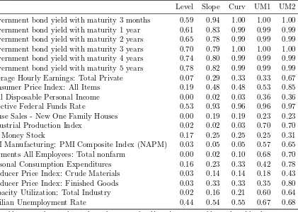
Table 10 reports the cumulative variance of yields and macro variables explained by the

macro-yields factors when identification restrictions are imposed on the macro factors. Comparing Table

10 with Table 2, we can notice that the imposition of the identification restrictions slightly changes

the proportion of variance explained by the macro factors. Table 11 shows that the correlation of the

first unspanned macro factor with the industrial production marginally increases from 91% to 92%

when the identification restrictions are imposed and the correlation of the second unspanned macro

Table 10: Cumulative variance explained by the macro-yields factors with identification

Level Slope Curv UM1 UM2

Government bond yield with maturity 3 months 0.59 0.94 1.00 1.00 1.00 Government bond yield with maturity 1 year 0.61 0.83 0.99 0.99 0.99 Government bond yield with maturity 2 years 0.65 0.78 0.99 0.99 0.99 Government bond yield with maturity 3 years 0.70 0.79 1.00 1.00 1.00 Government bond yield with maturity 4 years 0.74 0.80 0.99 0.99 0.99 Government bond yield with maturity 5 years 0.78 0.82 0.99 0.99 0.99 Average Hourly Earnings: Total Private 0.07 0.29 0.33 0.33 0.67 Consumer Price Index: All Items 0.19 0.48 0.48 0.53 0.85 Real Disposable Personal Income 0.00 0.02 0.03 0.36 0.36

Effective Federal Funds Rate 0.53 0.93 0.96 0.96 0.97

House Sales - New One Family Houses 0.00 0.19 0.19 0.23 0.23

Industrial Production Index 0.02 0.02 0.03 0.70 0.70

M1 Money Stock 0.17 0.25 0.25 0.25 0.31

ISM Manufacturing: PMI Composite Index (NAPM) 0.03 0.05 0.05 0.57 0.65 Payments All Employees: Total nonfarm 0.00 0.02 0.10 0.68 0.70 Personal Consumption Expenditures 0.16 0.23 0.33 0.42 0.78 Producer Price Index: Crude Materials 0.03 0.14 0.14 0.18 0.43 Producer Price Index: Finished Goods 0.03 0.33 0.33 0.35 0.80 Capacity Utilization: Total Industry 0.02 0.16 0.21 0.60 0.64

Civilian Unemployment Rate 0.44 0.54 0.55 0.67 0.68

This table reports the cumulative share of variance of yields and macro variables explained by the macro-yields factors when identification restrictions are imposed on the macro factors.

Table 11: Correlation of the factor estimates with the proxies

L S C UM1 UM2

MY 0.97 0.96 0.84 0.91 0.75 MY∗ _{0.97 0.96 0.84 0.92 0.72}

This table reports the correlation between the factor estimates with the corresponding prox-ies. The first row refers to the MY model without the identification restrictions, the sec-ond row MY∗ _{refers to the factor estimates}

G

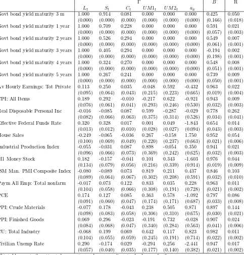
Estimated parameters

In Tables 12–13 we report the estimated parameters of the macro-yields model described in

Equa-tions 4-6. Standard errors are computed using a Monte Carlo procedure, as follows: we estimate

the macro-yields model in equations 4-6 and save the idiosyncratic innovations and the state

in-novations. We then bootstrap the state innovations and simulate the state variables. In the same

way, we bootstrap the idiosyncratic innovations and simulate the idiosyncratic components. We

then obtain a sample of artificial yields and macro variables by adding the simulated idiosyncratic

components to the simulated state variables multiplied by the estimated factor loadings. We

gen-erate a 1000 simulated samples of yields and macro variables and for each simulated sample we

estimate the macro-yields model. The standard deviations of parameters reported in Tables 12–13

are the standard deviations of the empirical distribution of each model parameter.

Results in Table 12 show that most macro variables have statistically significant factor loadings

on the level and slope of the yield curve. The autocorrelation coefficient in the idiosyncratic

components is significant for all variables, except for one yield. Results in Table 13 show that

the level is mainly Granger caused by the second unspanned macro factor, i.e. the real interest

rate. The slope and the curvature are mainly Granger caused by the first factor, i.e. industrial

Table 12: Estimated parameters: measurement equation

Γ B R

Lt St Ct U M1t U M2t ax

Govt bond yield maturity 3 m 1.000 0.914 0.081 0.000 0.000 0.000 0.425 0.050 (0.000) (0.000) (0.000) (0.000) (0.000) (0.000) (0.166) (0.018) Govt bond yield maturity 1 year 1.000 0.709 0.228 0.000 0.000 0.000 0.591 0.021

(0.000) (0.000) (0.000) (0.000) (0.000) (0.000) (0.057) (0.003) Govt bond yield maturity 2 years 1.000 0.526 0.294 0.000 0.000 0.000 0.549 0.007

(0.000) (0.000) (0.000) (0.000) (0.000) (0.000) (0.061) (0.001) Govt bond yield maturity 3 years 1.000 0.405 0.294 0.000 0.000 0.000 -0.194 0.002

(0.000) (0.000) (0.000) (0.000) (0.000) (0.000) (0.198) (0.001) Govt bond yield maturity 4 years 1.000 0.324 0.270 0.000 0.000 0.000 0.548 0.008

(0.000) (0.000) (0.000) (0.000) (0.000) (0.000) (0.051) (0.001) Govt bond yield maturity 5 years 1.000 0.267 0.241 0.000 0.000 0.000 0.739 0.009

(0.000) (0.000) (0.000) (0.000) (0.000) (0.000) (0.050) (0.001) Av Hourly Earnings: Tot Private 0.113 0.250 0.035 -0.048 0.592 -0.432 0.963 0.022

(0.095) (0.064) (0.043) (0.215) (0.223) (0.665) (0.019) (0.004) CPI: All Items 0.189 0.292 -0.010 -0.217 0.622 -0.921 0.943 0.009

(0.076) (0.061) (0.041) (0.293) (0.246) (0.530) (0.032) (0.003) Real Disposable Personal Inc -0.016 -0.085 0.087 0.599 -0.287 -0.029 0.778 0.262

(0.082) (0.066) (0.063) (0.375) (0.314) (0.526) (0.034) (0.041) Effective Federal Funds Rate 0.320 0.328 0.017 0.001 0.049 -1.843 0.654 0.014

(0.013) (0.012) (0.010) (0.028) (0.027) (0.094) (0.043) (0.003) House Sales -0.249 -0.065 -0.036 0.267 -0.158 1.750 0.952 0.054

(0.100) (0.069) (0.049) (0.220) (0.237) (0.663) (0.021) (0.006) Industrial Production Index -0.055 -0.031 0.087 0.898 -0.054 0.350 0.941 0.021

(0.096) (0.066) (0.073) (0.369) (0.242) (0.625) (0.032) (0.003) M1 Money Stock 0.182 -0.157 -0.041 0.101 0.343 -1.603 0.976 0.044

(0.134) (0.079) (0.056) (0.216) (0.339) (0.914) (0.019) (0.009) ISM Man. PMI Composite Index -0.080 -0.089 0.073 0.819 0.211 0.437 0.846 0.103

(0.089) (0.064) (0.067) (0.302) (0.208) (0.591) (0.032) (0.010) Paym All Emp: Total nonfarm -0.017 0.073 0.122 0.833 0.035 0.228 0.963 0.011

(0.104) (0.058) (0.066) (0.308) (0.191) (0.728) (0.021) (0.002)

PCE 0.174 0.127 0.085 0.363 0.578 -1.092 0.797 0.086

(0.091) (0.060) (0.047) (0.174) (0.171) (0.687) (0.033) (0.008) PPI: Crude Materials -0.077 0.178 -0.043 0.238 0.505 0.871 0.897 0.144

(0.098) (0.083) (0.058) (0.306) (0.310) (0.675) (0.030) (0.021) PPI: Finished Goods 0.069 0.296 -0.023 -0.191 0.732 -0.028 0.907 0.024

(0.084) (0.068) (0.047) (0.340) (0.284) (0.563) (0.041) (0.006) CU: Total Industry -0.068 0.199 0.069 0.642 0.117 0.823 0.982 0.011

(0.104) (0.055) (0.059) (0.245) (0.191) (0.714) (0.022) (0.002) Civilian Unemp Rate 0.290 -0.174 0.029 -0.294 0.256 -2.441 0.947 0.017

(0.057) (0.040) (0.035) (0.177) (0.140) (0.382) (0.021) (0.002) This table reports the estimated parameters and corresponding standard errors for the measurement

Table 13: Estimated parameters: state equation

A µ Q

Lt₋₁ St₋₁ Ct₋₁ U M1t₋₁ U M2t₋₁

Lt 0.998 0.013 -0.004 -0.020 0.051 0.029 0.055 0.050 0.034 0.004 -0.032

(0.010) (0.010) (0.014) (0.024) (0.023) (0.064) (0.019) (0.024) (0.050) (0.016) (0.021) St -0.016 0.966 0.025 0.144 0.032 0.049 0.050 0.102 -0.054 0.017 -0.040

(0.022) (0.017) (0.022) (0.050) (0.039) (0.159) (0.024) (0.049) (0.076) (0.032) (0.041) Ct 0.033 0.030 0.889 0.155 0.078 -0.221 0.034 -0.054 0.750 -0.079 -0.007

(0.037) (0.038) (0.048) (0.079) (0.071) (0.248) (0.050) (0.076) (0.241) (0.077) (0.070) U M1t 0.005 -0.038 0.006 0.996 0.007 -0.106 0.004 0.017 -0.079 0.032 0.000

(0.009) (0.023) (0.019) (0.014) (0.016) (0.074) (0.016) (0.032) (0.077) (0.020) (0.015) U M2t 0.002 0.009 -0.012 0.009 0.979 -0.004 -0.032 -0.040 -0.007 0.000 0.035

H

Alternative macro dataset

This Appendix contains results using an alternative macroeconomic dataset. Following Banbura,

Giannone, Modugno and Reichlin (2012), we aim at selecting the headline macroeconomic variables.

Accordingly, the series we collect are marked on Bloomberg website as Market Moving Indicators.

We only include the headlines of each macroeconomic report since these are the data followed by

financial markets and extensively commented by the newspapers. Table 14 contains a complete

list of the macroeconomic variables along with the transformation applied to ensure stationarity.

We transform all the variables in annual growth rates, except for the federal funds rate, the

unem-ployment rate, housing starts, houses sold, Philadelphia Fed. survey, conference board consumer

confidence and the PMI manufacturing index which we keep in levels. The monthly U.S. Treasury

zero-coupon yield curve data are the same as in the main text.

Table 14: Macroeconomic variables in the alternative dataset

Series N. Mnemonic Description Transformation

1 IP Industrial Production Index 1

2 PMI ISM Manufacturing: PMI Composite Index (NAPM) 0

3 PI Real Disposable Personal Income 1

4 Unem Civilian Unemployment Rate 0

5 Paym Payments All Employees: Total nonfarm 1

6 PCE Personal Consumption Expenditures Price Index 1

7 Hstat Housing Starts 0

8 Hsold House Sales - New One Family Houses 0

9 PPI Producer Price Index: Finished Goods 1

10 CPI Consumer Price Index for All Urban Consumers 1

11 FFR Effective Federal Funds Rate 0

12 Imp Imports 1

13 Exp Exports 1

14 Phil Philadelphia Fed. Survey, General business activity 0

15 CB Conference Board, Consumer confidence 0

16 RS Sales of retail stores 1

17 NORD Mfrs’ new orders durable goods industries 1

This table lists the alternative 17 macro variables used to estimate the macro-yields. Most series have been transformed prior to the estimation, as reported in the last column of the table. The transformation codes are: 0 = no transformation and 1 = annual growth rate.

Table 15: Model selection with the alternative dataset

Number of factors IC∗ _V

3 0.10 0.49

4 -0.07 0.31

5 -0.11 0.23

6 -0.02 0.19

7 0.13 0.17

8 0.36 0.16

This table reports the information cri-terion I C∗_{, and the sum of the}

vari-ance of the idiosyncratic components (divided by N T), V, when different numbers of factors are estimated.

dataset. Table 15 indicates that two unspanned factors are necessary in order to capture the

comovement of yields and the alternative macro variables. Table 16 shows that the yield curve

factors explain most of the variance of the yields and the federal funds rate. They also explain

part of the variance of price indices and unemployment. The first unspanned macro factor captures

the dynamics of industrial production and other real variables, while the second unspanned factor

mainly explains prices, as with our original dataset. Figure 2 shows that the first unspanned

macroeconomic factor closely tracks the industrial production index, with a correlation of 92%,

and the second unspanned macroeconomic factor proxies the real interest, with a correlation of

74%. Also the out-of-sample results, reported in Table 17, are in line with the results obtained

Table 16: Cumulative variance of yields and macro variables explained by the macro-yields factors

Level Slope Curv UM1 UM2 Government bond yield with maturity 3 months 0.59 0.96 1.00 1.00 1.00 Government bond yield with maturity 1 year 0.61 0.84 0.99 0.99 0.99 Government bond yield with maturity 2 years 0.65 0.79 0.99 0.99 0.99 Government bond yield with maturity 3 years 0.70 0.79 1.00 1.00 1.00 Government bond yield with maturity 4 years 0.74 0.80 1.00 1.00 1.00 Government bond yield with maturity 5 years 0.78 0.82 1.00 1.00 1.00

Industrial Production Index 0.04 0.04 0.04 0.68 0.68

ISM Manufacturing: PMI Composite Index (NAPM) 0.06 0.08 0.08 0.63 0.66 Real Disposable Personal Income 0.00 0.04 0.04 0.36 0.46

Civilian Unemployment Rate 0.47 0.56 0.58 0.61 0.62

Payments All Employees: Total nonfarm 0.01 0.02 0.08 0.64 0.65 Personal Consumption Expenditures Price Index 0.13 0.20 0.29 0.47 0.57

Housing Starts 0.14 0.14 0.14 0.47 0.48

House Sales - New One Family Houses 0.44 0.47 0.52 0.55 0.54 Producer Price Index: Finished Goods 0.04 0.36 0.36 0.37 0.63 Consumer Price Index for All Urban Consumers 0.20 0.52 0.52 0.53 0.70

Effective Federal Funds Rate 0.55 0.98 1.00 1.00 1.00

Imports 0.01 0.04 0.05 0.22 0.48

Exports 0.02 0.19 0.20 0.26 0.46

Philadelphia Fed. Survey, General business activity 0.02 0.18 0.18 0.53 0.53 Conference Board, Consumer confidence 0.15 0.15 0.15 0.37 0.51

Sales of retail stores 0.05 0.18 0.18 0.53 0.56

Mfrs’ new orders durable goods industries 0.03 0.04 0.04 0.65 0.65

This table reports the cumulative share of variance of yields and alternative macro variables explained by the macro-yields factors. The first three columns refer to the yield curve factors (level, slope and curvature) and the last two to the unspanned macroeconomic factors (U M1 andU M2).

Table 17: Out-of-sample performance with the alternative dataset

Macro-Yields

Maturity 3m 1y 2y 3y 4y 5y

h=1 0.85 0.99 1.10 1.08 1.12 1.18 h=3 0.79 0.96 1.07 1.08 1.12 1.14 h=6 0.77 0.91 1.02 1.05 1.07 1.09 h=12 0.73 0.78 0.85 0.89 0.91 0.93 h=24 0.76 0.70 0.73 0.77 0.81 0.89

Figure 2: Macro-yields factors with the alternative dataset

80 90 00 4 6 8 10 12 14

Level vs. NS

80 90 00 -6 -4 -2 0 2 4 6

Slope vs. NS

80 90 00 -6 -4 -2 0 2 4 6 8 10

Curvature vs. NS

80 90 00 -3 -2 -1 0 1 2

UM1 vs. IP

Model Proxy

80 90 00 -2

-1 0 1 2

UM2 vs. r

I

Alternative dataset with more yields

This appendix reports results with an alternative dataset that contains more yields than macro

variables. We use a dataset composed by 17 yields (3 month and six month yields from CRSP, and

1 to 15 year yields from G¨urkaynak, Sack and Wright (2007)) and 5 macro variables(Consumer Price

Index, Industrial Production Index, Payments All Employees, Personal Consumption Expenditures

and Producer Price Index: Finished Goods). Table 18 shows that also with this dataset the

information criterion selects the model with two unspanned macro factors. Table 19 shows that the

first three factors capture most of the variation in the 17 yields included in this dataset and that

the two unspanned macro factors are mainly related to industrial production (the first) and the

component in prices that is not explained by the yield curve factors (the second). The top plots

Figure 3 compare the two unspanned macro factors obtained from the macro-yields model with the

unrestricted macro factors obtained from the macro-yields model without imposing the unspanning

restriction. The two set of factors are very close. This provides evidence that the zero restrictions

on the factor loadings are satisfied also by this dataset and that the macro factors are unspanned

by the cross-section of yields. This happens because yields have a strong factor structure and they

can be fully characterized by a very small number of common factors, regardless of the number of

yields considered in the analysis. As a final robustness check, the bottom plot of Figure 3 compare

the unspanned macro factors obtained with this alternative dataset with the unspanned macro

factors obtained in the paper. The extracted factors are very similar to the ones extracted in the

paper. The only difference is that the factors extracted with the dataset proposed by the referee

are more volatile, reflecting the less precise extraction of the factors due to the smaller number of

Table 18: Model selection with more yields

# of factors IC* V

3 -0.84 0.19 4 -0.65 0.17 5 -0.87 0.11 6 -0.66 0.10

This table reports the information criterion I C∗ _{and the sum of the}

variance of the idiosyncratic com-ponents (divided byN T_),V_{, when} different numbers of factors are es-timated.

Table 19: Cumulative variance of yields and macro variables explained by the macro-yields factors

Level Slope Curv UM1 UM2

Figure 3: Estimated macro factors

80 90 00

-2 -1 0 1 2

Unspanned Macro 1 vs Macro 1

MY UMY

80 90 00

-2 -1 0 1 2

Unspanned Macro 2 vs Macro 2

MY UMY

80 90 00

-2 -1 0 1 2

Unspanned Macro 1: different datasets

MY MY(paper)

80 90 00

-2 -1 0 1 2

Unspanned Macro 2: different datasets

MY MY(paper)

J

Only-yields model with a unit root in the level

Duffee (2011) finds that imposing a unit root restriction on the level factor results in superior yield

predictions. To compare our results with this type of models, we estimate a only-yields version of

our model with a unit root in the level factor. This is a restricted version of the macro-yields model

in equations 4-6 withQyx=Ayx= Γxy = 0 and the parameters in the state equation are restricted as follows

µy =

0 µS µC

and Ayy =

     

1 0 0

0 ASS ACS 0 ASC ACC

     

The out-of-sample forecasting performance of this model is reported in Table 20. Comparing

these results with the ones in Table 5, we can notice that imposing random walk dynamics to the

level of interest rates improves the predictive ability of the only-yield model in the long horizon.

However this model is not able to outperform neither the macro-yields model neither the random

walk.

Table 20: Out-of-sample performance

Only-yields model with unit root in the level

Maturity 3m 1y 2y 3y 4y 5y

h=1 0.99 1.29 1.23 1.14 1.11 1.15 h=3 1.03 1.27 1.26 1.19 1.15 1.18 h=6 1.04 1.28 1.30 1.27 1.22 1.24 h=12 0.97 1.11 1.19 1.22 1.21 1.23 h=24 0.82 0.85 0.92 0.99 1.03 1.10

K

Recursive model selection

In this Appendix we report the out-of-sample performances of the macro-yields model and the

block-diagonal macro-yields model when the number of macro factors is selected every time the

model is re-estimated.

As explained before, we estimate the model at the beginning of each year of our evaluation

sample. Given that we report the performances up to two-year horizon, the first time the model

is estimated is in January 1988 (with this parameters we produce the two-year ahead forecast for

January 1990). Table 21 shows that while for the block-diagonal macro-yields model there is some

instability in the selection of the number of macro factors, prior to 2000, the macro-yield model is

stable: the information criterium selects always 5 factors. This result leads to a slight deterioration

of the out-of-sample performances for the block diagonal model, see Table 22, probably due to the

fact that for 1998 and 1999 the number of factors selected is equal to eight. For the macro-yields

model the out-of-sample performances are equal to the ones reported in the main text, given that

the number of factors selected is always equal to five.

Table 21: Model selection for the block-diagonal and the macro-yields model

Number of factors year Block-diagonal Macro-yields

1988-1992 5 5

1993 6 5

1994-1997 4 5

1998-1999 8 5

2000-2008 6 5

Table 22: Out-of-sample performance with recursive model selection

Macro-Yields Model

Maturity 3m 1y 2y 3y 4y 5y

h=1 1.17 1.05 1.06 1.00 1.05 1.14

h=3 0.79* 0.93 0.99 0.96 0.99 1.02

h=6 0.78** 0.89 0.94 0.93 0.93 0.94

h=12 0.69** 0.74** 0.79** 0.80*** 0.80*** 0.80*** h=24 0.62*** 0.66*** 0.74** 0.82** 0.88* 0.97

Block-diagonal Macro-yields Model

Maturity 3m 1y 2y 3y 4y 5y

1 0.90 1.14 1.10 1.06 1.03 1.08

3 0.85* 1.04 1.08 1.04 1.03 1.04

6 0.76** 0.95 1.03 1.02 1.00 1.00

12 0.70*** 0.84* 0.95 0.99 0.99 1.01

24 0.87 0.93 1.07 1.17 1.25 1.36

References

Banbura, Marta, Domenico Giannone, Michele Modugno, and Lucrezia Reichlin (2012) ‘Now-casting and the real-time data flow.’ Handbook of Economic Fore‘Now-casting, G. Elliott and A. Timmermann, eds., Volume 2, Elsevier-North Holland

Diebold, Francis X, and Canlin Li (2006) ‘Forecasting the term structure of government bond yields.’Journal of Econometrics 130, 337–364

Duffee, Gregory R (2011) ‘Forecasting with the term structure: The role of no-arbitrage restric-tions.’ Technical Report, Working papers//the Johns Hopkins University, Department of Eco-nomics

G¨urkaynak, Refet S, Brian Sack, and Jonathan H Wright (2007) ‘The us treasury yield curve: 1961 to the present.’ Journal of Monetary Economics54(8), 2291–2304

Ludvigson, Sydney C, and Serena Ng (2009) ‘Macro factors in bond risk premia.’Review of Finan-cial Studies 22(12), 5027

M¨onch, Emanuel (2012) ‘Term structure surprises: The predictive content of curvature, level, and slope.’ Journal of Applied Econometrics27(4), 574–602