Stochastic injection-strategy optimization for the preliminary assessment of candidate
geological storage sites
Brent M. Cody1*, Domenico Baù2, Ana González-Nicolás3 1. Natural Resources Consulting Engineers, [email protected] 2. University of Sheffield, Sheffield, UK
3. Colorado State University, Fort Collins, CO, USA *corresponding author
Keywords: Climate Change, Analytical Models, Multi-objective Optimization, Carbon Sequestration
Hydrogeology Journal, 23 (6). 1229 -1245. ISSN 1431-2174
Published online 25 April 2015: DOI 10.1007/s10040-015-1250-54.
Abstract
1 Introduction
Geological carbon sequestration (GCS) has been identified as a prominent technology to manage increasing atmospheric concentrations of carbon dioxide (CO2) (Nordbotten and Celia 2012, Pacala and
Socolow 2004), however, the effective application of GCS will require a global implementation of large numbers of carbon injection projects. While an individual large coal-fired power plant may emit up to 5-10 megatonnes (Mt) of CO2 per year (Birkholzer et al. 2012), total annual global anthropogenic carbon emissions measured in mass of CO2 are approximately 30,000 Mt (Nordbotten and Celia 2012). Results from Eccles et al. (2012) suggest that specific regions of a small number of candidate aquifers will provide the majority of low cost geological CO2 storage. As the selection of the appropriate reservoir is crucial to the success of a GCS project (Bossie-Codreanu and Le Gallo 2004), many potential injection sites will need to be assessed world-wide for GCS suitability. Therefore, the efficient preliminary characterization of candidate GCS injection sites has the potential for massive resource savings. In addition, a comprehensive pre-screening effort will increase GCS storage reliability by eliminating “bad” and identifying “good” GCS reservoirs.
The high computational cost associated with numerical models may be reduced by the use of data-based response surface methods (e.g. Box and Draper 2007). However, it is the authors’ intent for the resulting
framework to ultimately be used to optimize and compare large numbers of potential injection sites having vastly different domain characteristics. Creating and calibrating each potential injection site’s
numerical model, as well as training the resulting response surface would require user expertise and large investments of computational time. This work has therefore chosen to use a semi-analytical multiphase flow model presented by Nordbotten et al. (2009) for multiphase subsurface flow simulation. The semi-analytical leakage algorithm is very general and can be applied to simplified computational models of the vast majority of potential injection sites.
An additional difficulty associated with preliminary GCS project planning is that potential storage reservoirs typically exhibit a high degree of uncertainty associated with physical parameters. Celia et al. (2011) identified abandoned (herein referred to as “passive”) well permeabilities as the most dominant uncertainty parameter when estimating fluid leakage due to GCS. In North America, significant numbers of passive wells may perforate the caprock in formations suitable for GCS (Celia et al. 2009, Nogues and Dobossy 2012, Nordbotten and Celia 2012). Most likely, very little information exists on the location and/or sealing properties of these wells. However, several efforts have been made to investigate and account for the uncertainty associated with passive well permeability. Watson and Bachu (2008; 2009) developed a passive well integrity scoring index based upon typically available information (e.g. completion date, regulatory requirements, etc.). Crow et al. (2009) physically sampled and analyzed segments of a 30 yr. old passive well that had been continuously exposed to 96% CO2 finding that cement interfaces are more important than the cement matrix when quantifying migration pathways.
find best performing injection strategies that maximize the mass of CO2 sequestered while minimizing project cost by selecting optimal injection well locations and injection rates. In multi-objective problems,
a Pareto-optimal, or non-dominated, solution outperforms all other solutions with respect to all objectives (Reed 2013). Multi-objective evolutionary algorithms (MOEAs) have been shown to be effective in
providing Pareto-optimal solutions for a large number of subsurface flow applications possessing several decision variables (Alzraiee et al. 2013,Baú 2012, Chen et al. 2007, Hansen et al. 2013, Kumphon 2013, Mantoglou and Kourakos 2006, Nicklow et al. 2010, Peralta et al. 2014, Reed and Kollat 2013, Singh 2013, Singh 2014, Singh and Chakrabarty 2010, Tabari and Soltani 2012, Zheng, F., Zecchin 2014). In particular, (Reed 2013) presents a comprehensive review of state-of-the-art MOEAs highlighting key algorithm advances which may be used to identify critical tradeoffs in water resources problems. A
non-dominated sorting genetic algorithm (NSGA-II; Deb et al. 2002) with ε-dominance (Laumanns et al. 2002) has been selected as the computational optimization tool because it is among the most reliable and
best performing multi-objective optimization evolutionary algorithms (Cheng et al. 2009).
2011, Viswanathan et al. 2008, Wagner and Gorelick 1987, Wriedt et al. 2014). In particular, Celia et al. (2011) applied a stochastic Monte Carlo approach to estimate leakage risk associated with passive well
permeability uncertainty. Nogues and Dobossy (2012) used a large-scale Monte Carlo method to explore the effects of caprock permeability uncertainty on fluid leakage estimation, finding that the amount of
CO2 leakage from GCS is typically acceptable for climate change mitigation.
Herein, several computational tools are integrated into a stochastic multi-objective optimization framework for the purpose of performing large-scale GCS site feasibility studies. These tools include 1) a semi-analytical leakage algorithm to rank the performance of trial injection strategies; 2) a Monte Carlo
procedure to quantify risk resulting from parameter uncertainty; and 3) a NSGA-II with ε-dominance
(Deb et al. 2002) to heuristically determine Pareto-optimal solutions between competing objectives. The paper begins with a detailed description of the stochastic optimization methodology including an
overview of both the semi-analytical CO2 leakage algorithm and the NSGA-II with ε-dominance. Next, a
2 Methodology
2.1 Semi-Analytical CO2 Leakage Estimation
While other semi-analytical algorithms provide insight regarding specific processes, this work has chosen
to use a modified version of the ELSA (Estimating Leakage Semi-analytically) multiphase subsurface flow model (Nordbotten et al. 2009, Celia et al. 2011). This model has been used in several applications
(Nogues and Dobossy 2012, Bielicki et al. 2013 & 2014) because it is the only semi-analytical model able to simulate multiphase flow in domains having multiple injection wells, geological layers, and passive wells (i.e. weak caprock areas).
Figure 1 shows a schematic of the semi-analytical leakage model’s computational domain. This domain is structured as a stack of L+1 caprock layers separated by L aquifer layers, perforated by M carbon injection wells and N passive wells. Aquifers are assumed to be horizontally level, homogenous, and isotropic. Caprock layers are assumed to be impermeable, except where perforated by passive wells. Injection wells are able to inject into any layer. Initially, fluid is not flowing through any of the passive wells because the entire domain is assumed to be saturated with brine at hydrostatic pressure. Additional assumptions made by this model include: a) aquifers exhibit horizontal flow; b) capillary pressure is negligible, resulting in a sharp CO2-brine interface; c) CO2 plume thickness at any given location is assumed to be the maximum plume thickness from all sources and sinks in the aquifer; d) pressure response from sources and sinks can be superimposed in each aquifer; and e) the injectivity of the formation remains constant. Several of these processes are important (Cihan et al. 2013, Court et al. 2012, Doster et al. 2013, Gasda et al. 2011, Gasda et al. 2012, Heße et al. 2013, Juanes et al. 2009) and should be included (Buscheck et al. 2012, Gasda et al. 2009, Huang et al. 2014, Nordbotten and Flemisch
At the start of injection, aquifer fluid pressures throughout the domain begin to change resulting in pressure differentials across caprock layers and fluid flux through passive wells. It is therefore very
important to understand aquifer fluid pressure response resulting from changes in the mass storage of CO2 and brine. A pressure response function for the injection of CO2 into a brine-filled confined aquifer was
derived by Nordbotten and Celia (2005). Celia et al. (2011) expresses this radial pressure response p
[ML-1T-2] at the bottom of the aquifer where a single well injects CO 2 as:
𝑝=𝑝!+ 𝜌!−𝜌! ∙𝑔∙𝐻∙∆𝑝! (1)
where p0 is the initial fluid pressures at the bottom of the aquifer, 𝜌! is fluid density [ML-3] (αdenotes the
phase type, b for brine and c for CO2), 𝑔 is gravitational acceleration [LT-2] and 𝐻 is aquifer thickness [L]. In Eqn (1), ∆𝑝! (/) is defined by:
∆𝑝! 𝜒 =
0 for 𝜒≥𝜓
− 1 2𝛤ln
𝜒
𝜓 +∆𝑝! 𝜓 for𝜓>𝜒≥2𝜆 1
𝛤− 𝜒
𝛤 2𝜆+∆𝑝
! 2𝜆 +𝐹 ℎ! for 2𝜆>𝜒≥2 𝜆
− 1
2𝜆𝛤ln
𝜒𝜆
2 +∆𝑝!
2
𝜆 for
2
𝜆>𝜒
(2)
where,
𝜒 =2𝜋𝐻𝜙 1−𝑆!
!"# 𝑟!
𝛤=2𝜋 𝜌!−𝜌! 𝑔𝑘𝐻
!
𝜇!𝑄 (4)
𝜓=4.5𝜋𝐻𝜙𝑘 1−𝑆!
!"#
𝜇!𝑐!""𝑄 (5)
ℎ!=ℎ(𝜒)
𝐻 =
1 𝜆−1
2𝜆
𝜒 −1 (6)
𝐹(ℎ′)= −𝜆
𝜆−1 ℎ′−
𝑙𝑛 𝜆−1 ℎ′+1
𝜆−1 (7)
In Equations (2-7): B is aquitard thickness [L]; h is CO2 plume thickness [L]; h’ [/] is the CO2 plume
thickness relative to the aquifer thickness H; 𝑆!!"# is the residual saturation of the brine [/]; t is time [T]; k
is the aquifer permeability [L2]; µ is the dynamic viscosity [ML-1T-1];φ is the aquifer porosity [/]; Q is the
total volumetric well flux [L3T-1]; c
eff is the effective compressibility of the fluid and solid matrix [M -1LT2]; and r is the radial distance [L]. Also, F(h’) is an offset term related to the vertical pressure
distribution (Celia et al. 2011) and the mobility ratio is defined as λ = λc/λb, where λα= kr,α/µα and kr,α is the
relative permeability of phase α (α = b for brine or α = c for CO2).
To determine the fluid overpressure at any given time throughout the aquifer system, Nogues and Dobossy (2012) applied superposition of effects derived from the application of Eqn (1) for all the volumetric sources and sinks corresponding to CO2 injection wells and passive wells. Consequently, the
𝑝!,! =𝑝!!+ 𝜌!−𝜌! ∙𝑔∙𝐻!∙ ∆𝑝! 𝜒 !",!,! !
!"!!
+ ∆𝑝! 𝜒 !,!,! !
!!!
(8)
where
𝜒!",!,! =
2𝜋𝐻!𝜙! 1−𝑆!,!"#! 𝑟!"!,!
𝑄!",!∙𝑡 (9)
and
𝜒!,!,!=2𝜋𝐻!𝜙! 1−𝑆!,!"#! 𝑟!,!! 𝑄!,!−𝑄!,!!! ∙𝑑𝜏
!
!
(10)
By following this approach, the fluid pressures at the bottom of each aquifer and at each passive well can be grouped into the N×L vector 𝐩:
𝐩(t)=𝐩 𝐏𝟏,𝐌(t) (11)
Eqn (11) shows that 𝐩(t) is a function of the array
𝐏!≡ 𝐇,𝛟,𝐤,𝑺!!"#,𝐫 ,𝐐
!",𝜌!,𝜌!,𝑔,𝜆,𝜋,𝜇!,𝑐!"" (12)
In Eqn (12): the L×1 vectors H, 𝛟, 𝑺!!"#and k include the thicknesses, porosities, brine residual
aquifer l (l=1,2,..,L) for injection well iw (iw=1,2,..,M); and the (M+N)×(M+N) r matrix includes the
relative distances between injection and passive wells.
In addition, 𝐩(t) (Equation 9) is a function of the N×L vector 𝐌(t), whose generic component 𝑀!,!(𝑡)
represents the net cumulative fluid mass transferred into aquifer l through passive well j. This mass is
calculated as:
𝑀!,! 𝑡 = 𝜌!"",!,! 𝜏 ∙ 𝑄!,! 𝜏 −𝑄!,!!! 𝜏 ∙𝑑𝜏
!
!
(13)
where 𝜌!"",!,! 𝜏 is the effective fluid density in aquifer 𝑙, at passive well 𝑗 which is time-dependent since
the leaking fluid composition is a function of the phase saturations of CO2 and brine, which vary based on
the CO2 plume location. The effective fluid density is estimated as 𝜌!"",!,! =𝜌!∙𝑆!!,!+𝜌!∙ 1−𝑆!!,! .
Since application of Eqn (11) requires knowing the temporal evolution of leakage rates through passive
wells 𝑄!,!, Nogues and Dobossy (2012) propose to use the sum of the flow rates, 𝑄!!,!, for each phase α,
calculated using the multiphase version of Darcy’s law across each confining layer l for each passive well
j:
𝑄!,! = 𝜋𝑟!"! !,!
𝑘!,!!,!𝑘!"!,!
𝜇!𝐵! 𝑝!,!!!−𝜌!𝑔𝐵!−𝑔𝜌!𝐻!!!−𝑝!,!
!!!,!
(14)
In Eqn (14), 𝑟!"!,! is the passive well radius and 𝑘!"!,! is the single phase passive well permeability for
well as CO2 relative thicknesses in passive well pathways, must be known to estimate pressure gradients, fluid saturations and relative permeability values. Given Eqn (14), the flow rates across each aquitard l
(l=1,2,..,L) for each passive well j (j=1,2,..,N) can be can be grouped into the N×L vector 𝐐:
𝐐(t)=𝐐 𝐏𝟐,𝐩(t) (15)
where the array 𝐏! is given by:
𝐏!≡ 𝐁,𝐇,𝐫!",𝐤!",𝐤!,!,𝐤!,!,𝜌!,𝜌!,𝜇!,𝜇!,𝑔 (16)
In Eqn (16), the (L+1)×1 vector 𝐁 includes the aquitard thicknesses, the N×(L+1) matrices 𝐫!" and
𝐤!"contain the passive well radii and permeabilities, and the N×(L+1) matrices 𝐤!,!and 𝐤!,! include the
relative permeabilities of CO2 and brine at passive wells.
By combining Equations (9) and (13), a set of N∙L non-linear equations in N∙L unknowns is obtained. These unknowns are the fluid pressures at the bottom of each aquifer and at each passive well (Equation 8), and the flow rates (Equation 12) across each aquitard for each passive well.
In an effort to increase computational efficiency, this work has chosen to neglect effects from upconing and apply an Iterative Global Pressure Solution (IGPS) modification where a fixed-point iteration scheme (Takahashi 2000) is applied to solve the system of non-linear equations introduced above at a generic
2.2 Stochastic Multi-objective GCS Problem
For any given potential GCS reservoir, a set of Pareto-optimal injection scenarios exist which (a)
maximize the deterministic mass of CO2 injected, Massinj, and (b) minimize the stochastic project cost, C,:
𝑜𝑏𝑗𝑒𝑐𝑡𝑖𝑣𝑒 𝑎 : max Mass!"# 𝐐 (17)
𝑜𝑏𝑗𝑒𝑐𝑡𝑖𝑣𝑒 𝑏 : min 𝐶 𝐱,𝐐,𝐬 (18)
In Eqns (17-18), spatial position, x, and flow rate, Q, are the two decision variables comprising each
injection strategy and 𝐬 is the set of stochastic state variables (i.e. aquifer pressure distribution and CO2 plume locations and thicknesses) dependent on each simulation’s injection strategy and stochastic parameter set. Massinj is simply the total mass of CO2 injected into the domain during simulation, and is calculated by multiplying the sum of injection well flow rates by the injection duration, tinj:
Mass!"#= 𝑄!!"∗𝑡!"# !
!"!!
(19)
where M is the number of injection wells, and 𝑄!!"is the CO2 mass injection rate for injection well iw.
Note that the project cost, C, is a stochastic variable and is here estimated using a Monte Carlo (MC) simulation based on a stochastically generated parameter set. In order to quantify the risk of CO2 leakage associated with uncertain aquifer permeability, effective compressibility, and passive-well segment
permeability, an ensemble of NMC parameter set realizations [(𝐤(!), 𝐤(!), … , 𝐤(!!")), (𝐜!""(!), 𝐜𝐞!!(!), … ,
each trial injection strategy. For each parameter realization, aquifer permeabilities and effective compressibilities are assigned a value using log-normal distributions. Each passive-well segment is
assigned either an “intact” (low) or “degraded” (high) (Celia et al. 2011, Nogues and Dobossy 2012) permeability value. This is accomplished using a simple bi-value probability distribution function (PDF).
Passive-well segments have a Pintact chance of being assigned an “intact” permeability value and a (1 -
Pintact) chance of being assigned a “degraded” permeability value. The cost, Costi, associated with each MC realization, i (i = 1,2,…,NMC), consists of the summation of each injection well’s (iw) capital cost, Cap, operational cost, OP, surface maintenance cost, SurM, subsurface maintenance cost, SubM, and variable cost, Var, added to the cost associated with CO2 leakage, LC:
Cost!(𝐐,Mass!"#$)
= Cap!"+OP!"(𝑡!"#)+ SurM!"(𝑡!"#)+SubM!"(𝑡!"#) !
!"!!
+Var!"(𝑄!",𝑡!"#) +LC[Mass!"#$(𝐐,𝐬!)]
(20)
where si is the set of state variables for each MC realization including the CO2 saturation and total flow rate in each passive-well segment. LC is estimated as:
LC[Mass!"#$(𝐐,𝐬!)]=𝑐!∙Mass!"#$(𝐐,𝐬!)!! (21)
Mass!"#$(𝐐,𝐬!)= 𝜌!∙𝑆!!,!! 𝑡 ∙𝑄!,!(!)(𝑡)∙𝑑𝑡 !!"#
! !
!!!
(22)
Empirical cumulative distribution functions (CDFs) of each injection strategy’s MC Cost (Cost1, Cost2, … , CostNMC) are then compiled by first sorting the Cost vector in ascending order from i = 1…NMC, then
assigning the non-exceedance probability of Costi as (i – 0.5)/NMC (Hahn and Shapiro 1967). The stochastic cost objective, C, is finally assigned as the zth percentile value, Pz, of the sorted Cost vector:
𝐶 𝐱,𝐐,𝐬 =𝑃!(𝐂𝐨𝐬𝐭) (23)
As discussed later in Section ‘NSGA-II parameter calibration’, larger NMC values are needed to accurately quantify C as z becomes farther from 50%. Several constraints are included in this problem. First, the number of injection wells is limited to a maximum integer value by constraining M to a value between 0 and Mmax:
0≤𝑀≤𝑀!"# (24)
All candidate injection wells must be located horizontally within prescribed minimum and maximum spatial bounds representing the areal extent selected for the construction of GCS faculties:
𝑥!"# ≤𝑥!"≤𝑥!"#; 𝑦!"# ≤𝑦!" ≤𝑦!"# ; iw=1,2,..,𝑀 (25)
Also, each injection well’s flow rate must be between prescribed minimum and maximum flow rates Qmin
𝑄!"# ≤𝑄!"≤𝑄!"# ; iw=1,2,..,𝑀 (26)
In Eqn (26), Qmin and Qmax are physical constraints related to the technical capacity of injection pumps and wells. Finally, down-hole fluid pressures at each injection well in each layer, piw,l, must not exceed each layer’s fracture fluid pressure, 𝑝!"#$!.
𝑝!",! 𝐐,𝐬 <𝑝!"#$! ; iw=1,2,..,𝑀;𝑙=1,2,..,𝐿 (27)
where 𝑝!"#$! is calculated by multiplying a specified fracture gradient (Celia et al. 2011) by the layer
depth and piw,l is estimated for each injection well iw at the end of the injection duration at a small effective distance from the injection location. The value for effective distance must be carefully selected as Eqn (1) is very sensitive to radial distance when estimating pressure changes nearby the injection location. A conservative estimate for this value would be the injection well’s casing radius. Note that because the left-hand side of Eqn (27) contains stochastic state variables, these stochastic constraints have
to be transformed into deterministic. This is carried out using a chance-constraint approach (Wagner and Gorelick 1987) such that:
Prob 𝑝!",! 𝐐,𝐬 <𝑝!"#$! ≥𝑆!; iw=1,2,..,𝑀 ;𝑙 =1,2,..,𝐿 (28)
Eqn (28) requires the probability of the fluid pressure at injection wells not exceeding the layer fracture pressure to be larger than or equal to a prescribed fracture safety probability, Sp.
2.3 Multi-objective GCS Optimization Algorithm
Leakage Estimation’) and the Monte Carlo procedure (Section ‘Stochastic Multi-objective GCS Problem’)
are integrated into a NSGA-II with ε-dominance. Each trial injection strategy is encoded into a
“chromosome” (i.e. a unique sequence of binary numbers representing the values of each decision variable). The first segment of the chromosome contains spatial location information for Mmax injection wells represented by Ncl predefined candidate injection-well location indices, thus intrinsically satisfying the spatial location constraint defined by Eqn (25). The number of digits required to represent each injection well’s location is a function of the number of candidate locations, Ncl. For example, if Ncl = 16 for a potential GCS site, the locational information of each injection well for each injection strategy would require four binary digits (i.e. ‘0000’ = 1, ‘0001’ = 2, … , ’1111’=16). In this case, the spatial data component of the chromosome has a length of M∙4. The last segment of the chromosome represents the injection rate index of each candidate well. Injection rate indices represent Nir prescribed discrete flow rate values within the constraints of Eqn (26). For example, injection rate index values of 0, 1, 2, 3, and 4 may represent injection rates of 0, 20, 30, and 40 kg/s, respectively (Nir = 4). In this case, two binary digits would be used to encode each well’s injection index (‘00’ = 0, ‘01’ = 1, … , ’11’=3) bringing the
total chromosome length to M∙4 + M∙2.
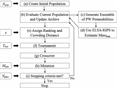
The general procedure followed by the NSGA-II with ε-dominance is presented in Figure 2. Once input
for each of these realizations in step (d), then objective values Massinj and 𝐶 are calculated using Equations (16-20). Also in step (d), if Eqn (28) is violated the injection strategy is deemed infeasible.
Next, the NSGA-II is used to generate new injection strategy populations of size Npop using selection, crossover, and mutation operators. In step (e), population members are first ranked (irank) as the number of solutions dominating population member i using the fast non-dominated sorting procedure (Deb et al. 2002), and then assigned a crowding distance (idistance) as the largest cuboid in objective space enclosing the point i without including any other point in the population (Deb et al. 2002). A partial order is established using the crowding comparison operator, ≥n (Deb et al. 2002). Population member i
outperforms member j if the following conditions are met:
𝑖 ≥! 𝑗 IF 𝑖!"#$ < 𝑗!"#$ OR 𝑖!"#$= 𝑗!"#$ AND 𝑖!"#$%&'(> 𝑗!"#$%&'( (29)
The NSGA-II’s ranking process is further improved with the concept of ε-dominance (Laumanns et al.
2002). Suppose population members p1 and p2 have fitness values of f1 and f2, respectively. Using ε
-dominance, p1 is allowed to dominate p2 if (1+ε)∙f1is greater than or equal to f2. The ε-dominance allows
for the inclusion of additional, well-performing population members to each rank’s Pareto-optimal front.
Next, in step (f), an iterative tournament-style selection process is used to select parent injection strategies
chance, quantified as the mutation rate, Mrate, in which chromosome elements of this new population will be randomly altered during step (h). Steps (b-h) are repeated until the maximum prescribed number of
generations, Ngens, is reached.
2.4 Efficient Computational Implementation
This framework utilizes parallel computing and simulation archiving to improve the computational efficiency. Due to the iterative nature of both evolutionary search and Monte Carlo analyses, large numbers of model simulations are needed for each stochastic optimization run. Without using simulation archiving, the total number of model calls required for each stochastic optimization run, Nct, is equal to the product of NMC, Npop, and Ngens. CO2 leakage estimation calculations for each trial injection strategy are independent and therefore may be processed in parallel (i.e. simultaneously) rather than sequentially by distributing processes on different computer cores.
3 Characterization of the Michigan Basin test site
The Michigan Basin (MB) is near the town of Thompsonville in northwest Michigan. Michigan
Technological University’s data library provides detailed subsurface data in this region. A cross-sectional schematic of the MB is provided in Figure 3 along with a map of the study area, showing a nearly
depleted hydrocarbon reservoir between depths of approximately 4660 and 5000 feet (1420-1520 meters) overlain by multiple confining and saline aquifer layers. This reservoir’s only production well, Merit 1-20A, was originally drilled by the Shell Oil Company and is located between two exploration boreholes, Burch 1-20B and Stech 1-21A. This work explores the simulation and optimization of GCS into the saline Grey Niagaran formation immediately below the hydrocarbon reservoir.
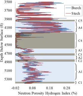
The Burch 1-20B (Burch) and Stech 1-21A (Stech) boreholes have provided a wide variety of high resolution well logs that may be used to characterize subsurface domain properties such as density, porosity, electrical resistivity, and compressional and shear wave velocities. For this analysis, neutron porosity hydrogen index (NPHI) data were used, gathered from the boreholes to estimate aquifer and caprock locations, thicknesses, and permeabilities. High NPHI values indicate relatively high permeability while regions exhibiting low NPHI values indicate low permeability caprock layers. Figure 4 shows NPHI versus depth for both the Burch and Stech boreholes. Aquifer (highlighted light blue) and caprock (highlighted brown) layers are then defined using this data. Derived formation thicknesses and depths shown in Figure 4 correspond with aggregated layer sets displayed in Figure 3.
at passive well locations. Average aquifer permeability, k, in milliDarcys (mD; 1 mD ≅ 10-15 m2) is estimated for all aquifer layers using the following from Trebin (1945):
𝑘= 2∙𝑒!".!∙! 𝑖𝑓 𝜙<0.124
4.94∙10!∙𝜙!−763 𝑖𝑓 𝜙≥0.124 (30)
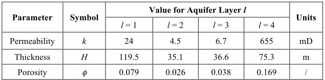
where, φ is assumed to equal NPHI. Table 1 shows the permeability, thickness, and porosity value for
[image:20.612.70.400.363.445.2]each aquifer layer obtained using the preceding methodology.
Table 1 Aquifer permeability, thickness, and porosity values used in this study
Parameter Symbol Value for Aquifer Layer l Units
l = 1 l = 2 l = 3 l = 4
Permeability k 24 4.5 6.7 655 mD
Thickness H 119.5 35.1 36.6 75.3 m
Porosity φ 0.079 0.026 0.038 0.169 /
The Michigan Department of Environmental Quality maintains a database of producing and inactive oil and gas wells in the state. Although 65,560 well records containing permit number, depth, and spatial coordinates are retrieved from the department’s website (Michigan Department of Environmental Quality Oil and Gas Database 2014), only 131 wells are located within 4 km of the reservoir’s production well, Merit 1-20A, and intersect the four aquifer layers defined above.
may be selected from 16 candidate locations uniformly distributed over a 2.25 km2 square grid. Figure 5 provides a plan view of the MB site with candidate injection well locations (Ncl = 16) shown as orange
circles and existing passive well locations (N = 131) shown as blue pluses. Horizontal positions are relative to the Merit 1-20 production well with xmin= ymin = -750 m and xmax = ymax = 750 m), thereby satisfying constraint Eqn (25).
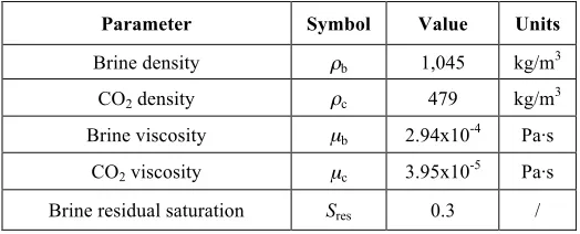
[image:21.612.71.333.432.538.2]In Eqn (21), Massleak is defined as the cumulative mass of CO2 that escapes into the top layer (l = 4) at the end of the 50-year injection duration. The radius, rpw, used in Eqn (14) is assumed to be 0.2 m for all 131 passive wells. A fracture safety probability of Sp = 95% is assumed for the pressure constraint (Eqn (28)). Also a fracture gradient of 14.2 kPa/m (Oldenburg et al. 2011) is used for this analysis. Table 2 lists additional deterministic hydrogeological parameter values used herein.
Table 2 Deterministic hydrogeological parameter symbols and values
Parameter Symbol Value Units
Brine density ρb 1,045 kg/m3
CO2 density ρc 479 kg/m3
Brine viscosity µb 2.94x10⁻⁴ Pa·s
CO2 viscosity µc 3.95x10⁻⁵ Pa·s
Brine residual saturation Sres 0.3 /
Headwaters Clean Carbon Services LLC, personal communication, 2012). The leakage cost parameter cL in Eqn (21) is assigned a values of 0.6 $/kg.
Table 3 Cost parameter values for each candidate well location in Eqn (20)
Capital Cost, Cap ($/well) Fixed O&M Cost, OP ($/day/well) Surface Maintenance, SurM ($/yr/well) Subsurface Maintenance, SubM ($/yr/well) Variable Cost, Var ($/kg of CO2)
3,537,104 11,566 120,608 37,612 0.009
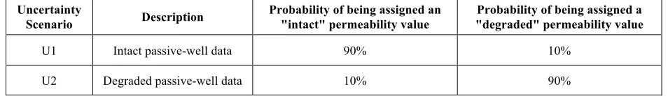
As stated previously, aquifer permeability, effective compressibility, ceff, and passive-well segment permeability are assumed to be uncertain variables. For each MC simulation, aquifer permeabilities and effective compressibilities are assigned a random value using log-normal distributions with a standard
deviation of 0.4, mean aquifer permeabilities from Table 1, and mean ceff of 4.6x10⁻¹⁰ m2/N (Celia et al. 2011). Passive-well segment permeabilities are randomly assigned as either 0.01 or 1000 mD,
representing “intact” and “degraded” cement, respectively (Celia et al. 2011, Court et al. 2012, Nogues and Dobossy 2012). Table 4 shows the probability of each passive-well segment being assigned an "intact" or “degraded” permeability value during the MC ensemble generation for each uncertainty scenario. Herein, two uncertainty scenarios are tested and compared including 1) data supporting an abundance of intact passive-well segments (U1) and 2) data supporting an abundance of degraded passive-well segments (U2). Passive-well segment permeabilities are assumed to be fully uncorrelated (i.e. passive wells may have differing permeabilities at different depths).
Table 4 Probability of passive-well segments being assigned either an "intact" or “degraded” permeability value for each
uncertainty scenario.
Uncertainty
Scenario Description
Probability of being assigned an "intact" permeability value
Probability of being assigned a "degraded" permeability value
U1 Intact passive-well data 90% 10%
[image:22.612.67.544.607.676.2]4 Results and Discussion
4.1 NSGA-II Parameter Calibration
The number of Monte Carlo simulations, NMC, generated and simulated for each trial injection strategy is
determined from an analysis of the uncertainty scenario U2. U2 is assumed to be the worst case (i.e. most difficult to solve) optimization problem because it has the largest probability of degraded passive wells
and, therefore, the greatest potential for CO2 leakage. Both P50%(Cost) and P95%(Cost) (Eqn (23)) are estimated for ten different injection strategies (Nsims = 10). For each of these simulations, the value of
NMC is ranged between 50 and 1000 in intervals of 50. An inspection of the results of this analysis shows that a NMC value of 400 produces convergence for both P50%(Cost) and P95%(Cost).
Optimal NSGA-II parameter values of Npop, Mrate, Tsize, and ε are selected from a series of preliminary
tests using a simplified deterministic optimization problem having 50% degraded and 50% intact passive-well segments. A deterministic problem is used because it requires much less computational time for
A performance comparison between the NSGA-II and a completely random search of the decision space is also performed to further validate the effectiveness of the NSGA-II used in this study. One hundred
deterministic optimization trials having differing random number seeds are processed. The genetic algorithm is found to greatly outperform the random search algorithm. The percent of trials reaching 0.1%
of the minimal project cost per unit mass sequestered in 200 generations is 100% for the NSGA-II compared to 0% for the random search algorithm. Results from this convergence test provide strong evidence that, for this problem, optimal or close-to-optimal Pareto sets are found using the algorithmic parameter set shown in Table 5.
Table 5 NSGA-II parameter values and maximum number of optimization generations used for the stochastic case study. All
parameters are dimensionless.
Npop Mrate Tsize ε Ngens
25 1.6% 2 0.001 200
4.2 Stochastic Optimization Analysis
Three goals regarding the stochastic optimization of the MB site are investigated and discussed within this section: 1) quantify the impact of DM preferences on heuristically determined Pareto-optimal
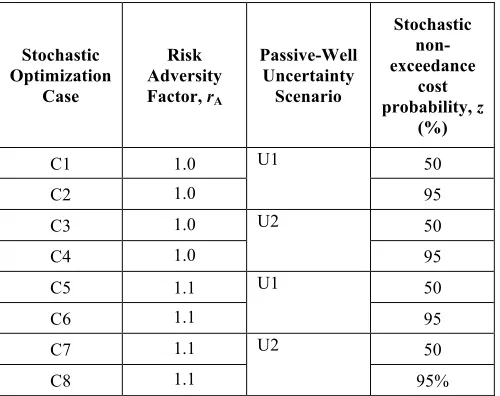
probability, z, is set to either 50% or 95% for each of the two possible passive-well uncertainty scenarios (U1, U2), hence obtaining a total of 2∙2∙2 = 8 combinations of DM preference selections. Table 6 shows DM preferences for each of these stochastic optimization cases (C1-C8).
Table 6 Decision maker (DM) preferences for each of the eight stochastic optimization runs (C1-C8)
Stochastic Optimization
Case
Risk Adversity Factor, rA
Passive-Well Uncertainty Scenario Stochastic non-exceedance cost probability, z
(%)
C1 1.0 U1 50
C2 1.0 95
C3 1.0 U2 50
C4 1.0 95
C5 1.1 U1 50
C6 1.1 95
C7 1.1 U2 50
C8 1.1 95%
4.2.1 Impact of DM Preferences on Objective Function Values
The first step in investigating relationships between DM preferences and objective function values is to
determine Pareto-optimal (or close-to-optimal) tradeoff sets for each stochastic optimization case described in Table 6 using the methodology presented in Section ‘Methodology’. The quantity of total
A visual representation of resulting Pareto sets is provided in Figure 6, where project cost versus mass of
CO2 sequestered is displayed for each of the 8 optimization cases described in Table 6. Figures 6a-d plot the objective function tradeoff curve associated with each uncertainty scenario (i.e. U1 and U2) for given
values of rA and z. Capital, operation and maintenance (CO&M) costs, defined herein as all project costs other than the penalties incurred from CO2 leakage, are also plotted. Policies found to violate the fracture constraints (Eqn (28)) are infeasible and are therefore not shown in Figure 6. Note that, due to higher project costs, a larger scale is used on the ordinate axis when rA = 1.1.
A general trend exhibited by these tradeoff profiles shows that project cost increases with the mass of CO2 sequestered in all optimization runs. A sharper increase in capital project cost is observed in CO&M costs when rA = 1.0 (Figure 6a-b) because, due to the maximum prescribed injection rate (Eqn (26)), an additional injection well is needed when sequestering more than 63.1 Mt of CO2. While increases in injection well capital costs are also incurred when rA = 1.1 (Figure 6c-d), they are overshadowed by much larger total project costs, as increasing rA drastically increase leakage penalty costs.
The selection of uncertainty scenario (Table 4) represents a DM’s knowledge of the GCS site’s caprock integrity. Uncertainty scenario selection directly impacts the estimated mass of CO2 leakage and,
therefore, indirectly affects the estimated cost associated with CO2 leakage. Cases assigned uncertainty scenarios having greater percentages of intact well segments are found to exhibit less CO2 leakage. All
optimization cases assigned a U1 uncertainty scenario exhibit fairly negligible CO2 leakage costs as their minimized total project costs are very similar to CO&M costs. There is, however, one exception to this observation: the fracture constraint (Eqn (28)) does not allow for any well to operate at 40 kg/s and therefore forces the installation of additional injection wells when sequestering more than 47.3 Mt of CO2
Finally, the choice of stochastic non-exceedance cost probability, z, affects the estimated cost associated with CO2 leakage because greater project costs are required to increase non-exceedance probability. Data shown in Figure 6 suggest that the value chosen for z has a minor impact on resulting Pareto-optimal objective function values, thus indicating that spread of each Cost CDF is relatively contained. Estimated project costs increase when a greater value of z is used. However, the project cost variability associated with stochastic non-exceedance cost probability is much smaller than the project cost variability associated with risk adversity or uncertainty scenario selection.
4.2.2 Impact of DM Preferences on Injection Strategy Selection
The impact of DM preferences upon the heuristic selection of optimal injection locations and flow rates is also investigated. Figure 7 displays a close-up, plan view of the MB test site showing the 16 candidate injection-well location indices.
As explained in Section ‘Impact of DM Preferences on Objective Function Values’, there are 12 possible mass sequestered values for each of the 8 optimization cases. Hence, for this problem there is a
However several of these solutions are rendered infeasible by the fracture constraints (Eqn (28)) and therefore not displayed in the following discussion. As a general presentation of decision variable results,
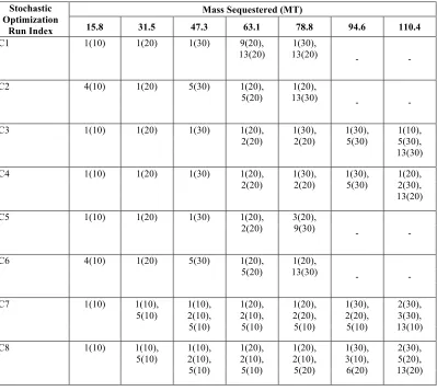
Table 7 shows both candidate well location indices (see Figure 7) and injection rates in kg/s for each injection strategy. Note that injection strategies may use multiple injection wells.
Table 7 Candidate well location indices from Figure 7 and injection rates for each injection, displayed as Location(Injection
Rate). Policies indicated as "-" are infeasible due to a violation of the fracture constraints (Eqn (28)).
Stochastic Optimization
Run Index
Mass Sequestered (MT)
15.8 31.5 47.3 63.1 78.8 94.6 110.4
C1 1(10) 1(20) 1(30) 9(20),
13(20) 13(20) 1(30), - -
C2 4(10) 1(20) 5(30) 1(20),
5(20)
1(20),
13(30) - -
C3 1(10) 1(20) 1(30) 1(20),
2(20) 1(30), 2(20) 1(30), 5(30) 1(10), 5(30),
13(30)
C4 1(10) 1(20) 1(30) 1(20),
2(20) 1(30), 2(20) 1(30), 5(30) 1(20), 2(30),
13(20)
C5 1(10) 1(20) 1(30) 1(20),
2(20)
3(20),
9(30) - -
C6 4(10) 1(20) 5(30) 1(20),
5(20) 13(30) 1(20), - -
C7 1(10) 1(10),
5(10) 1(10), 2(10), 5(10) 1(20), 2(10), 5(10) 1(20), 2(20), 5(10) 1(30), 2(20), 5(10) 2(30), 3(30), 13(10)
C8 1(10) 1(10),
5(10) 1(10), 2(10), 5(10) 1(20), 2(10), 5(10) 1(20), 2(10), 5(20) 1(30), 3(10), 6(20) 2(30), 5(20), 13(20)
Using the data presented in Table 7, two quantitative analyses are performed to study how DM preferences ultimately influence the heuristic selection of carbon injection strategies. First, the relative
[image:28.612.79.478.213.570.2]injection-well rate/location combinations divided by the total number of injection-well rate/location combinations in each comparison set. Optimization cases having all but one identical DM preferences are
individually compared. When contrasting rA (rA=1.0 with rA =1.1) a set of four injection strategy comparisons are made; stochastic optimization cases C1-C4 are thus compared with cases C5-C8,
respectively. Four injection strategy comparisons are also made when contrasting z (z=50% with z=95%); case C1 with case C2, case C3 with case C4, case C5 with case C6, and case C7 with case C8. Finally, a set of four injection strategy comparisons are made when contrasting uncertainty scenario (U1 with U2); cases C1-C2 are compared with cases C3-C4, respectively, and cases C5-C6 are compared with cases C7-C8, respectively. The percentage of injection strategies that remain constant when varying values of rA, uncertainty scenario, and values of z is quantified as 49.3%, 37.5%, and 58.3%, respectively. These findings are used to augment the following discussion.
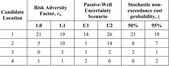
[image:29.612.76.370.594.709.2]Secondly, a categorical distribution analysis is used to identify general injection strategy trends associated with DM preferences. The number of times each candidate location is selected for injection-well placement is counted for all cases having each given DM preference value. For example, candidate location 1 is found to be selected for well placement 21 times when rA=1.0 (i.e. for cases C1-C4), 14 times when assuming uncertainty scenario U1 (i.e. for cases C1, C2, C5, and C6) and 21 times when z=50% (i.e. for cases C1, C3, C5, C7). Table 8 provides the number of selections of each candidate injection location for each DM preference value.
Table 8 Number selections for each candidate well location index. Indices having zero selections are not shown.
Candidate Location
Risk Adversity Factor, rA
Passive-Well Uncertainty Scenario
Stochastic non-exceedance cost
probability, z
1.0 1.1 U1 U2 50% 95%
1 21 19 14 26 21 19
2 5 10 1 14 8 7
3 0 3 1 2 2 1
5 5 12 4 13 7 10
6 0 1 0 1 0 1
9 1 1 2 0 2 0
13 5 3 4 4 4 4
15 0 0 0 0 0 0
16 0 0 0 0 0 0
Total 38 50 28 60 44 44
From the results shown in Table 8, the southwest corner of the candidate injection-well field is heavily favored by the optimization algorithm, regardless of parameter choice, with 81.8% of all injection-well placements being made at either candidate location 1, 2, or 5. This is due to the presence of a passive-well cluster approximately 1000 meters northeast of the candidate injection-passive-well field (see Figure 5). Also, the furthest southwest candidate injection-well location is found to have a substantially greater number of selections than all other individual locations. Approximately 45.5% of all injection-well placements are being made at candidate location 1, compared with 17.0% and 19.3% for candidate locations 2 and 5, respectively.
Passive-well uncertainty scenario selection is found to have the lowest percentage (37.5%) of injection strategy selections remaining constant, and therefore the greatest effect upon injection strategy selection
(see fourth and fifth columns of Table 8). The total number of candidate well location selections is also found to increase from 28 for uncertainty scenario U1 to 60 for the more expensive uncertainty scenario
U2, further validating the trend found when studying risk adversity. Also, greater estimated CO2 leakage, as in the case of uncertainty scenario U2, is clearly observed to drive candidate injection-well location selections further southwest. The likelihood of selecting the three furthest southwest candidate locations (i.e. locational indices 1, 2, and 5) increases from 67.9% in cases assigned uncertainty scenario U1 to 88.3% in cases uncertainty scenario U2.
Finally, the stochastic non-exceedance cost probability, z, is found to have the highest percentage (58.3%) of injection strategy selections remaining constant and, therefore, has the least effect on injection strategy selection. In addition, there are very similar results shown in the sixth and seventh columns of Table 8 with the total number of candidate location selections being identical for both columns.
4.2.3 GCS Suitability Assessment for the MB test site
4.3 Computational Efficiency
It is interesting to note that the complete enumeration of this problem would require 34,800,000
simulation calls:
𝑁!"∙𝑁!"!!"#∙ 𝑁!"
𝑖 !!"#
!!!
=400∙5!∙ 16!
1!∙15!+ 16!
2!∙14!+ 16!
3!∙13! =34,800,000 (31)
Assuming that a numerical model would require one hour per simulation, the CPU time required to sequentially process 34,800,000 CO2 leakage evaluations without archiving would be approximately 3,973 years. Therefore, a semi-analytical algorithm and an NSGA-II optimization approach is used to make this problem computationally feasible. For the NSGA-II optimization parameters provided in Table 5, each optimization run requires 2,000,000 simulation model calls, Nct, to estimate CO2 leakage without archiving (e.g. Nct = NMC∙Npop∙Ngens = 400∙25∙200 = 2,000,000). Assuming that each semi-analytical simulation requires 1 second, the CPU time required to sequentially process 2 million CO2 leakage evaluations without archiving would be 23.2 days. The computational time required for this problem may also be reduced using parallel processing and archiving. For example, if 25 computer processor cores are available, setting the number of parallel processes to Npop will reduce this theoretical simulation evaluation time by 96% to 0.93 days. The actual CPU time required for a single optimization run with
NMC = 400, Npop = 25, and Ngens = 200 using 12 processor cores and employing both parallel processing and simulation archiving is approximately 1.04 days, or about six orders of magnitude less than the theoretical time required for the complete enumeration of this problem using a numerical model. These findings show that the use of the optimization algorithm is essential in providing the computational efficiency required when deriving the Pareto optimal set, particularly if the number of candidate locations,
5 Conclusions
A stochastic methodology for determining optimal GCS injection strategies has been presented, where a semi-analytical CO2 leakage algorithm and a Monte Carlo procedure were integrated into a NSGA-II with
ε-dominance. In an effort to show the applicability of this method to real world potential injection sites, the stochastic optimization framework has been used to assess a hypothetical GCS project at a Michigan Basin (MB) test site in northern Michigan, USA. Eight MB test site stochastic optimization cases having differing DM preferences were evaluated.
DM risk adversity preference was found to have a profound effect on project cost when the estimated mass of CO2 leakage was high. While all optimization cases that were assigned an “intact” uncertainty scenario exhibited very little CO2 leakage, substantial CO2 leakage masses were estimated for test cases
assigned a “degraded” uncertainty scenario, resulting in large leakage costs with high risk adversity. The choice of stochastic non-exceedance cost probability had only a minor impact on resulting Pareto-optimal
objective function values.
This work also discussed large gains in computational efficiency using semi-analytical modeling, NSGA-II optimization, parallel computing, and simulation archiving. The actual CPU time required for a typical
optimization run using 12 processor cores and employing both parallel processing and simulation archiving was approximately 1.04 days, or about six orders of magnitude less than the theoretical time
required for the complete enumeration of this problem using a numerical model.
Because of the large set of assumptions made by the semi-analytical CO2 leakage algorithm, this framework may only be used for initial site planning and characterization. After ‘coarse scale’ project planning has been completed using this stochastic optimization framework, more rigorous, although slower, numerical models should be used for final project development of individual potential injection sites. However, this tool has potential for initial carbon-sequestration project planning as well as initial screening and ranking of large sets of potential carbon sequestration sites.
Looking forward, there are several possible variations of the optimization framework which may be explored. For example, the injection duration may be included as a third decision variable in addition to location and flow rate of each injection well. In addition, the minimization of risk of cost exceedance may be included as a third objective function in addition to maximizing the mass of CO2 sequestered and minimizing the project cost. A multi-criteria decision analysis (MCDA) may also be performed upon the resulting Pareto-optimal sets of equations to quantify the importance of conflicting objectives and aid in the final selection of injection strategy selection. Finally, substantial gains in computational efficiency may be obtained by additional parallelization using large processor core clusters. Increased
References
Alzraiee, A.H., Bau, D.A., Garcia, L.A. (2013) Multiobjective design of aquifer monitoring networks for optimal spatial prediction and geostatistical parameter estimation. Water Resour. Res. 49, 3670–3684
Baú, D.A. (2012) Planning of groundwater supply systems subject to uncertainty using stochastic flow reduced models and multi-objective evolutionary optimization. Water Resour. Manag. 26, 2513–2536
Bielicki, J.M., Pollak, M.F., Fitts, J.P., Peters, C.A. (2014) Causes and financial consequences of geological CO2 storage reservoir leakage and interference with other subsurface resources. Int. J. Greenh. Gas Control. 20, 272–284
Bielicki, J.M., Pollak, M.F., Wilson, E.J., Fitts, J.P., Peters, C.A. (2013) A Method for monetizing basin-scale leakage risk and stakeholder impacts. Energy Procedia. 37, 4665–4672
Birkholzer, J.T., Cihan, A., Zhou, Q. (2012) Impact-driven pressure management via targeted brine extraction - Conceptual studies of CO2 storage in saline formations. Int. J. Greenh. Gas Control. 7, 168–180
Bossie-Codreanu, D., Le Gallo, Y. (2004) A simulation method for the rapid screening of potential depleted oil reservoirs for CO2 sequestration. Energy. 29, 1347–1359
Box, G., Draper, N. (2007) Response surfaces, mixtures, and ridge analyses, Second Edition. Wiley.
Buscheck, T.A., Sun, Y., Chen, M., Hao, Y., Wolery, T.J., Bourcier, W.L., Court, B., Celia, M.A., Julio Friedmann, S., Aines, R.D. (2012) Active CO2 reservoir management for carbon storage: Analysis of operational strategies to relieve pressure buildup and improve injectivity. Int. J. Greenh. Gas Control. 6, 230–245
Celia, M.A., Nordbotten, J.M., Bachu, S., Dobossy, M., Court, B. (2009) Risk of leakage versus depth of injection in geological Storage. Energy Procedia. 1, 2573–2580
Celia, M.A., Nordbotten, J.M., Court, B., Dobossy, M., Bachu, S. (2011) Field-scale application of a semi-analytical model for estimation of CO2 and brine leakage along old wells. Int. J. Greenh. Gas Control. 5, 257–269
Chen, L., McPhee, J., Yeh, W.W.-G. (2007) A diversified multiobjective GA for optimizing reservoir rule curves. Adv. Water Resour. 30, 1082–1093
Cheng, Y., Jin, Y., Hu, J. (2009) Adaptive epsilon non-dominated sorting multi-objective evolutionary optimization and its application in shortest path problem. ICCAS-SICE, 2009. 2545–2549
Cihan, A., Birkholzer, J.T., Zhou, Q. (2013) Pressure buildup and brine migration during CO2 storage in multilayered aquifers. Ground Water. 51, 252–67
Court, B., Bandilla, K.W., Celia, M.A., Janzen, A., Dobossy, M., Nordbotten, J.M. (2012) Applicability of vertical-equilibrium and sharp-interface assumptions in CO2 sequestration modeling. Int. J. Greenh. Gas Control. 10, 134– 147
Crow, W., Brian Williams, D., William Carey, J., Celia, M., Gasda, S. (2009) Wellbore integrity analysis of a natural CO2 producer. Energy Procedia. 1, 3561–3569
Doster, F., Nordbotten, J.M., Celia, M.A. (2013) Impact of capillary hysteresis and trapping on vertically integrated models for CO2 storage. Adv. Water Resour. 62, 465–474
Eccles, J.K., Pratson, L., Newell, R.G., Jackson, R.B. (2012) The impact of geologic variability on capacity and cost estimates for storing CO2 in deep-saline aquifers. Energy Econ. 34, 1569–1579
Espinet, A.J., Shoemaker, C.A. (2013) Comparison of optimization algorithms for parameter estimation of multi-phase flow models with application to geological carbon sequestration. Adv. Water Resour. 54, 133–148
Gasda, S.E., Nordbotten, J.M., Celia, M.A. (2009) Vertical equilibrium with sub-scale analytical methods for geological CO2 sequestration. Comput. Geosci. 13, 469–481
Gasda, S.E., Nordbotten, J.M., Celia, M.A. (2011) The impact of local-scale processes on large-scale CO2 migration and immobilization. Energy Procedia. 4, 3896–3903
Gasda, S.E., Nordbotten, J.M., Celia, M.A. (2012) Application of simplified models to CO2 migration and immobilization in large-scale geological systems. Int. J. Greenh. Gas Control. 9, 72–84
Goda, T., Sato, K. (2011) Optimization of well placement for geological sequestration of carbon dioxide using adaptive evolutionary Monte Carlo algorithm. Energy Procedia. 4, 4275–4282
Hahn, G.J., and Shapiro, S.S. (1967) Statistical models in engineering. John Wiley, New York
Hansen, A.K., Hendricks Franssen, H.-J., Bauer-Gottwein, P., Madsen, H., Rosbjerg, D., Kaiser, H.P. (2013) Well field management using multi-objective optimization. Water Resour. Manag. 27, 629–648
Heße, F., Prykhodko, V., Attinger, S. (2013) Assessing the validity of a lower-dimensional representation of fractures for numerical and analytical investigations. Adv. Water Resour. 56, 35–48
Huang, X., Bandilla, K.W., Celia, M.A., Bachu, S. (2014) Basin-scale modeling of CO2 storage using models of varying complexity. Int. J. Greenh. Gas Control. 20, 73–86
Juanes, R., MacMinn, C.W., Szulczewski, M.L. (2009) The footprint of the CO2 plume during carbon dioxide storage in saline aquifers: storage efficiency for capillary trapping at the basin scale. Transp. Porous Media. 82, 19– 30
Kumphon, B. (2013) Genetic Algorithms for Multi-objective Optimization: Application to a multi-reservoir system in the Chi River Basin, Thailand. Water Resour. Manag. 27, 4369–4378
Laumanns, M., Thiele, L., Deb, K., Zitzler, E. (2002) Combining convergence and diversity in evolutionary multiobjective optimization. Evol. Comput. 10, 263–82
Mantoglou, A., Kourakos, G. (2006) Optimal groundwater remediation under uncertainty using multi-objective optimization. Water Resour. Manag. 21, 835–847
The MathWorks, Inc. (2012) MATLAB and Statistics Toolbox Release 2012b. Natick, Massachusetts, United States
Michigan Department of Environmental Quality Oil and Gas Database (2014) http://www.michigan.gov/deq/0,4561,7-135-6132_6828-98518--,00.html Accessed 08 March 2014
Nicklow, J., Reed, P., Savic, D. (2010) State of the art for genetic algorithms and beyond in water resources planning and management. J. Water Resour. Plan. Manag. 412–432
Nogues, J., Dobossy, M. (2012) A methodology to estimate maximum probable leakage along old wells in a geological sequestration operation. Int. J. Greenh. Gas Control. 7, 39–47
Nordbotten, J., Celia M. (2012) Geological storage of CO2. Wiley
Nordbotten, J., Celia, M. (2005) Semi-analytical solution for CO2 leakage through an abandoned well. Environ. Sci. Technol. 39, 602–611
Nordbotten, J., Celia, M., Bachu, S. (2004) Analytical solutions for leakage rates through abandoned wells. Water Resour. Res. 40, 1–10
Nordbotten, J., Flemisch, B. (2012) Uncertainties in practical simulation of CO2 storage. Int. J. Greenh. Gas Control. 9, 234–242
Nordbotten, J., Kavetski, D., Celia, M., Bachu, S. (2009) Model for CO2 leakage including multiple geological layers and multiple leaky wells. Environ. Sci. Technol. 43, 743–749
Oladyshkin, S., Class, H., Helmig, R., Nowak, W. (2011) An integrative approach to robust design and probabilistic risk assessment for CO2 storage in geological formations. Comput. Geosci. 15, 565–577
Oldenburg, C.M., Jordan, P.D., Nicot, J.-P., Mazzoldi, A., Gupta, A.K., Bryant, S.L. (2011) Leakage risk assessment of the In Salah CO2 storage project: Applying the certification framework in a dynamic context. Energy Procedia. 4, 4154–4161
Pacala, S., Socolow, R. (2004) Stabilization wedges: solving the climate problem for the next 50 years with current technologies. Science. 305, 968–972
Peralta, R.C., Forghani, A., Fayad, H. (2014) Multiobjective genetic algorithm conjunctive use optimization for production, cost, and energy with dynamic return flow. J. Hydrol.
Reed, P.M., Hadka, D., Herman, J.D., Kasprzyk, J.R., Kollat, J.B. (2013) Evolutionary multiobjective optimization in water resources: The past, present, and future. Adv. Water Resour. 51, 438–456
Reed, P.M., Kollat, J.B. (2013) Visual analytics clarify the scalability and effectiveness of massively parallel many-objective optimization: A groundwater monitoring design example. Adv. Water Resour. 56, 1–13
Singh, A. (2013) Simulation and optimization modeling for the management of groundwater resources. I: Distinct applications. J. Irrig. Drain. Eng. 1–10
Singh, A. (2014) Simulation and Optimization Modeling for the Management of Groundwater Resources. II: Combined Applications. J. Irrig. Drain. Eng. 1–9
Tabari, M.M.R., Soltani, J. (2012) Multi-objective optimal model for conjunctive use management using SGAs and NSGA-II models. Water Resour. Manag. 27, 37–53
Takahashi W. (2000) Nonlinear functional analysis: Fixed point theory and its applications. Yokohama Publishers, Yokohama
Trebin, F.A. (1945) Oil permeability of sandstone reservoirs. Gostoptekhizdat, Moscow
Turpening, R.M., Toksöz, M.N., Born, A.E., et al. (1992) Reservoir delineation consortium annual report. Massachusetts Institute of Technology, Cambridge
Viswanathan, H.S., Pawar, R.J., Stauffer, P.H., Kaszuba, J.P, Carey, J.W, Olsen, S.C., Keating, G.N., Kavetski, D., Guthrie, G.D. (2008) Development of a hybrid process and system model for the assessment of wellbore leakage at a geologic CO2 sequestration site. Environ. Sci. Technol., 2008, 42 (19), 7280-7286
Wagner, B., Gorelick, S. (1987) Optimal groundwater quality management under parameter uncertainty. Water Resour. Res. 23, 1162–1174
Walter, L., Binning, P., Oladyshkin, S. (2012) Brine migration resulting from CO2 injection into saline aquifers–An approach to risk estimation including various levels of uncertainty. Int. J. Greenh. Gas Control. 9, 495–506
Watson, T., Bachu, S. (2008) Identification of wells with high CO2 leakage potential in mature oil fields developed for CO2-enhanced oil recovery. SPE Symp. Improv. Oil Recover
Watson, T., Bachu, S. (2009) Evaluation of the potential for gas and CO2 leakage along wellbores. SPE Drill. Complet.
Wriedt, J., Deo, M., Han, W.S., Lepinski, J. (2014) A methodology for quantifying risk and likelihood of failure for carbon dioxide injection into deep saline reservoirs. Int. J. Greenh. Gas Control. 20, 196–211
FIGURES:
[image:39.612.108.506.331.632.2]Fig. 1 Schematic of the semi-analytical leakage model’s computational domain
(b)
Fig. 3 a Map of study area and b a cross-sectional schematic of the Michigan Basin with the simulated injection layer highlighted orange (modified with permission from Turpening et al. (1992))
[image:40.612.151.517.81.670.2]Fig. 4 Neutron porosity hydrogen index (NPHI) vs. depth for the Burch 1-20B (Burch) and Stech 1-21A (Stech) boreholes. Light
Fig. 5 Plan view of the Michigan Basin test site showing all pumping wells (PW) and candidate injection wells (IW) included in
Fig. 6a-d Optimal project costs versus mass of CO2 sequestered for the eight optimization runs described in Table 6. Policies