Bayesian System Identification of Nonlinear Dynamical Systems using a Fast MCMC Algorithm

White Rose Research Online URL for this paper:

http://eprints.whiterose.ac.uk/81829/

Proceedings Paper:

Green, P.L. (2014) Bayesian System Identification of Nonlinear Dynamical Systems using

a Fast MCMC Algorithm. In: Proceedings of ENOC 2014, European Nonlinear Dynamics

Conference. ENOC 2014, European Nonlinear Dynamics Conference, 6-11 July 2014,

Vienna, Austria. .

[email protected] https://eprints.whiterose.ac.uk/ Reuse

Unless indicated otherwise, fulltext items are protected by copyright with all rights reserved. The copyright exception in section 29 of the Copyright, Designs and Patents Act 1988 allows the making of a single copy solely for the purpose of non-commercial research or private study within the limits of fair dealing. The publisher or other rights-holder may allow further reproduction and re-use of this version - refer to the White Rose Research Online record for this item. Where records identify the publisher as the copyright holder, users can verify any specific terms of use on the publisher’s website.

Takedown

If you consider content in White Rose Research Online to be in breach of UK law, please notify us by

Bayesian System Identification of Nonlinear Dynamical Systems using a Fast MCMC

Algorithm

Peter L Green

∗

_{Department of Mechanical Engineering, University of Sheffield, Mappin Street, Sheffield, UK, S1}

3JD

Summary. This paper addresses the Bayesian parameter estimation of nonlinear, structurally dynamical systems. Specifically, it is concerned with Markov Chain Monte Carlo (MCMC) methods which, via the evolution of an ergodic Markov chain through the parameter space, allow one to generate samples from the posterior parameter distribution given by Bayes’ theorem. A version of the well-known Simulated Annealing algorithm is presented where, to reduce computational cost, the transition from prior to posterior distributions is controlled via the gradual introduction of data into the likelihood. A method is proposed which allows one to introduce data in a ‘smooth’ and continuous manner such that, while moving from prior to posterior, a constant change in Shannon entropy can be maintained. The performance of the algorithm is demonstrated on the parameter estimation of a nonlinear dynamical system.

Introduction

Within the context of this paper, the task of Bayesian inference involves assessing the plausibility of a set of model structures - as well as the parameters within each model - of structurally dynamical systems using a set of training data. It is well-established that both levels of inference (parameter estimation and model selection) can be achieved through the sequential application of Bayes’ theorem:

P(θ_{|D,M) =}P(D|θ,M)P(θ|M)

P(D|M) (1)

P(M|D) = P(D|M)P(M)

P(D) (2)

whereMrepresents a candidate model,θis a vector of parameters within that model andDis a set of training data. Suc-cessful evaluation of equation (1) gives a probability density function describing the plausibility of the parameter vectorθ conditional on the set of training dataDand the modelM- this is known as posterior parameter distribution. Successful evaluation of equation (2) gives a probability mass function across the set of competing model structures which, it can be shown, assigns overly-complex models relatively low probabilities. Owing to the size constraints of this paper, a thorough description of equations (1) and (2) will not be given here - for more information the reader can consult [1] where, within a similar context to the current work, a comprehensive description of such a Bayesian framework is given.

In the last 20 years the applicability of Bayesian inference has been substantially improved through the use of Markov chain Monte Carlo (MCMC) methods. MCMC involves the creation of an ergodic Markov chain whose stationary distri-bution is equal toP(θ_|D,M)such that, once the chain has converged, it can be used to generate samples from posterior parameter distributions with complex geometries. ‘Classical’ MCMC methods such as the Metropolis algorithm [2] and Hybrid Monte Carlo [3] can be used to address this first level of inference while, in the present-day, advanced algorithms such as Reversible Jump MCMC [4], Transitional MCMC [5], Asymptotically Independent Markov Sampling [6] and Nested Sampling [7] are also capable of addressing Bayesian model selection.

While undoubtedly powerful, MCMC methods tend to be rather expensive and, as such, can only be employed when computationally cheap models are used. The aim of the current paper is to present the author’s preliminary work into a new MCMC algorithm which is designed to address this issue.

Before proceeding it is necessary to define some notation: throughout this paperπ(θ_{)is used the denote the ‘target} distribution’ of the MCMC algorithm - this is the posterior parameter distribution from which one wishes to generate samples. Additionally, an asterisk is used to represent unnormalised target distributions whileZ’s are used to represent normalising constants (such that π(θ_{) = π}∗₍θ_{)/Z). Finally it should be noted that, for convenience, the posterior} parameter distribution has been written in the following form:

P(θ_{|D,M)∝exp(−JL(}θ_)−JP(θ₎₎ (3)

such thatJLis the negative log-likelihood andJP is the negative log-prior.

Simulated Annealing

globally optimum region of the parameter space). This is achieved by using the Metropolis algorithm to generate samples sequentially from a set of target distributions:

π∗

j = exp(−βjJL−JP) j= 1,2, ... (4)

whereβis usually referred to as the ‘temperature’ and, for sake of readability, all dependencies onθhave been dropped. The general concept is that, while the Markov chain is evolving, the temperature variable is increased from 0 to 1 such that the target distribution gradually changes from the prior to the posterior parameter distribution. It can be shown that, through the introduction of this gradual transition, the Markov chain is more likely to converge to the desired region of the parameter space in a reasonable amount of time.

The strictly increasing sequence of temperature values is usually referred to as the ‘annealing schedule’. Choice of annealing schedule is critical - annealing too fast increases the risk of becoming stuck in a local trap while annealing too slow will unnecessarily increase computational cost. In this paper it is hypothesised that an appropriate annealing schedule is one in which the information content - the Shannon entropy in this case - is varied at a constant rate. This is discussed more in the following sections.

Data Annealing

Equation (4) shows that, by increasing the temperature from 0 to 1, one is essentially increasing the influence of the like-lihood on the posterior. In [9] the author proposed that, rather than using the temperature variable, a similar effect could be realised by gradually increasing the number of data points included in the likelihood. The advantage of this method (named ‘Data Annealing’) was that it reduced the number of data points that would need to be generated by the model Mevery time a MCMC sample was generated, thus decreasing computational cost. The disadvantage is that annealing through the introduction of data points is a relatively blunt instrument - one has less control over the rate at which infor-mation is introduced than if one were to use Simulated Annealing.

The purpose of the current work is to address this issue. Specifically, it aims to propose a version of the Data Annealing algorithm where one is able to have complete control over the rate at which information is introduced into the target distribution.

Proposed Methodology

Annealing with Constant Entropy Variation

As stated previously, it is hypothesised here that the optimum annealing schedule is one in which the Shannon entropy of the target distribution is varied at a constant rate. This is similar to the concept of ‘annealing with constant thermodynamic speed’ that was proposed in [10].

With the aim of deriving a general expression which can be used for future variants of the Simulated Annealing algorithm, it is supposed here thatJLis some function of the temperatureβ which is yet to be defined. Throughout the following analysis the derivative ofJLwith respect toβis simply written asJL′.

Recalling that the target distribution is written asπ=π∗_{/ZwhereZ is the normalising constant, it is convenient at this}

point to derive the following properties:

dπ∗

dβ =−J

′

Lπ∗,

dZ

dβ =−ZE[J

′

L],

dπ

dβ =π(E[J

′

L]−JL′). (5)

The Shannon entropy of the target distribution is given by

S= lnZ+E[JL] +E[JP] (6)

such that the aim here is to evaluate

dS dβ =

d(lnZ)

dβ +

d(E[JL])

dβ . (7)

Using the properties in equation (5), the first term of equation (7) is:

d(lnZ)

dβ =−E[J

′

L] (8)

while the second term can be evaluated as follows:

d(E[JL]) dβ =

d dβ

Z

=

Z _d(J

Lπ)

dβ dθ (10)

= Z

πJ′

L+πJL(E[JL′]−JL′)θ (11)

=E[J′

L] +E[JL]E[JL′]−E[JLJL′]. (12)

Substituting into equation (7) one finds that

dS

dβ =E[JL]E[J

′

L]−E[JLJL′] (13)

=−Cor(JL, JL′). (14)

whereCor(JL, JL′)is used to represent the (unnormalised) correlation coefficient betweenJLandJL′.

Using∆Sto represent the desired change in entropy (as defined by the user) and bearing in mind that an increase inβ must induce a reduction in entropy (as one’s parameter uncertainty is reduced), one finds that new values ofβshould be selected according to:

βj+1=βj+

|∆S| Cor(JL, JL′)

(15)

subject to the condition that

βj< βj+1≤1 ∀j. (16)

It is re-emphasised here that equation (15) is a general expression which holds, regardless of the functional relationship betweenJLandβ. It is relatively easy to prove that, for ‘traditional’ Simulated Annealing whereJL(β) =βJL, equation (15) shows that new values ofβshould be selected according to

βj+1 =βj+

|∆S| βjVar(JL)

. (17)

Data Annealing with Constant Entropy Variation

Having derived equation (15), the final task is to create a version of Data Annealing where, through defining the appropri-ate relationship betweenJLandβ, an annealing schedule with constant entropy variation can be realised. It is suggested here that, for the situation wherendata points have already been introduced and the user wishes to introduce the next

(N−n)points,JLshould be defined as:

JL(β) = (

n

2 ln(2πσ

2

) + 1 2σ2

n X

i=1

∆x2 i

)

+β

(

N−n

2 ln(2πσ

2

) + 1 2σ2

N X

i=n+1

∆x2 i )

(18)

whereσis the likelihood standard deviation and∆xirepresents the difference between theith point of model output and theith point of training data. Combining this expression with equation (15) should allow the new data to be introduced with a constant variation in the Shannon entropy. Once the new data has been fully introduced then the user can either terminate the algorithm or choose to add additional data points.

It should be noted that the above definition ofJL is specifically for the case where an uncorrelated Gaussian prediction-error model has been used and where the likelihood standard deviation is treated as an unknown parameter.

Pseudo-Code

At thejth stage in the algorithm where, say, one is ‘annealing in’ the data points indexed fromntoN, the algorithm proceeds as follows:

Input: desired change in Shannon entropy∆S

• Generate samples fromπjusing the Metropolis algorithm

• Setβj+1according to equation (15)

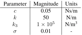
Parameter Magnitude Units c 0.05 Ns/m

k 50 N/m

k3 1×105 _N/m3

σ 0.01

-Table 1: Parameters used to generate training data.

0 50 100 150 200 250 300 350 400 450 500 −0.25

−0.2 −0.15 −0.1 −0.05 0 0.05 0.1 0.15 0.2 0.25

No. of Points

x

’Measured’ Response Actual Response

Figure 1: Time history training data.

– Setβj+1= 1

• Else ifβj = 1

– Prompt user to either terminate algorithm or add more training data

• End

Example using Simulated Data

Here the performance of the algorithm is demonstrated using a simple example: the parameter estimation of a SDOF nonlinear system using simulated time-history training data. The system of interest is a Duffing oscillator which is under a Gaussian white noise forcing:

¨

x+cx˙+kx+k3x3

=F (19)

wherexis displacement,F is the excitation force,c is viscous damping,k is linear stiffness andk3 is the nonlinear stiffness - the values of the parameters used are shown in Table 1. The ‘full’ set of training data consisted of 500 points of displacement measurements which had been artificially corrupted with Gaussian measurement noise of standard deviation

0.01. The resulting time history is shown in Figure 1.

With regards to the algorithm, it was decided that the training data should be introduced 100 points at a time (also shown in Figure 1). The parametersk,k3and the likelihood standard deviationσwere treated as being unknown. Gaussian prior distributions with standard deviation equal to 20,5×104_{and0.05were used fork,k3andσrespectively. For this simple} example the mean of each prior was set equal to the true parameter values. The desired change in the Shannon entropy was set equal to -1 and 1000 samples were generated at each iteration.

The resulting values ofβ are shown in Figure 2. It is interesting to note that, generally speaking, the initial sets of data have to be introduced in a gradual manner relative to the latter sets of training data. This is to be expected because, as more training data is used, the relative effect of an additional 100 points should be reduced.

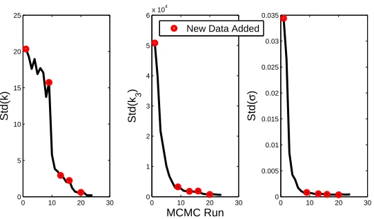
One of the advantages of the proposed algorithm is that it allows the user to monitor various properties as training data is added such that the algorithm can be terminated when certain criteria are met. As an example, Figures 3 and 4 show how, in the current case, the mean and standard deviation of the posterior parameter estimates varied as training data was added.

Can the Algorithm Fail ?

0 5 10 15 20 25 0 0.1 0.2 0.3 0.4 0.5 0.6 0.7 0.8 0.9 1 MCMC Run β

Figure 2: Variation ofβagainst the number of MCMC runs.

0 10 20 30 44 46 48 50 52 54 56 58 60 62 E[k]

0 10 20 30 0.99 1 1.01 1.02 1.03 1.04 1.05 1.06 1.07 1.08x 10

5

E[k

3

]

MCMC Run

0 10 20 30 0.01 0.015 0.02 0.025 0.03 0.035 0.04 0.045 E[ σ ]

New Data Added

Figure 3: Posterior mean of parameter estimates against the number of MCMC runs. Red circles represent the points where additional training data was added.

0 10 20 30 0 5 10 15 20 25 Std(k)

0 10 20 30 0 1 2 3 4 5 6x 10

4

Std(k

3

)

MCMC Run

0 10 20 30 0 0.005 0.01 0.015 0.02 0.025 0.03 0.035 Std( σ )

New Data Added

the posterior must be less than that of the prior:

E[Var(θ_{|D)] = Var(}θ_)−Var(E[θ_|D]). (20)

However, this result only states that additional data will reduce parameter uncertainty on average. Recalling equation (15), a reduction is Shannon entropy can only occur if the correlation betweenJL andJL′ is positive. This essentially means that, if additional data has the effect of increasing parameter uncertainty, then the algorithm will attempt to select a lower value ofβ(which is undesirable). While this has not occurred in the example shown here, it is an issue which the author aims to resolve as part of future work.

Conclusions

This paper presents a novel version of the well-known Simulated Annealing algorithm which can be used to aid the Bayesian system identification of structurally dynamical systems. It is based on the recently proposed Data Annealing algorithm, where the transition from prior to posterior is induced through the gradual introduction of training data (thus reducing computational cost). Presented here is a new version of Data Annealing which allows new training data to be introduced with a constant variation in the Shannon entropy.

Acknowledgements

This work was funded by the EPSRC Programme Grant ‘Engineering Nonlinearity’ EP/K003836/1.

References

[1] Beck, J.L., Katafygiotis, L.S. (1998) Updating models and their uncertainties. I: Bayesian statistical framework. Journal of Engineering Mechanics

124(4):455-461

[2] Rosenbluth, N., Rosenbluth, M.N., Teller, A.H., Teller, E. (1953). Equations of state calculations by fast computing machines. The Journal of Chemical Physics 21(6): 1087-1092

[3] Duane, S., Kennedy, A.D., Pendleton, B.J., Roweth, D. (1987) Hybird monte carlo. Physics letters B 195(2):216-222

[4] Green, P.J. (1995) Reversible jump Markov chain Monte Carlo computation and Bayesian model determination. Biometrika 82(4) 711-732 [5] Ching, J., Chen, Y.C. (2007) Transitional Markov chain Monte Carlo method for Bayesian model updating, model class selection, and model

averaging. Journal of engineering mechanics 133(7) 816-832.

[6] Beck, J.L., Zuev, K.M. (2013) Asymptotically independent Markov sampling: a new Markov chain Monte Carlo scheme for Bayesian inference. International Journal for Uncertainty Quantification 3(5).

[7] Skilling, J. (2006) Nested sampling for general Bayesian computation Bayesian Analysis 1(4) 833-859. [8] Kirkpatrick, S., Vecchi, M.P. (1983) Optimization by simmulated annealing. Science 220(4598) 671-680.

[9] Green, P.L. (2014) Bayesian System Identification of a Nonlinear Dynamical System using a Novel Variant of Simulated Annealing Mechanical Systems and Signal Processing Under Review