Detecting Damage on Wind Turbine Bearings Using Acoustic Emissions and Gaussian Process Latent Variable Models

COVER SHEET

NOTE:

 Please attach the signed copyright release form at the end of your paper and upload as a single ‘pdf’ file

 This coversheet is intended for you to list your article title and author(s) name only

 This page will not appear in the book or on the CD-ROM

Title: Detecting Damage on Wind Turbine Bearings using Acoustic Emissions and Gaussian Process Latent Variable Models

Authors: Ramon Fuentes, Thomas Howard, Matt B. Marshall, Elizabeth J. Cross, Rob Dwyer-Joyce, Tom Huntley, Rune H. Hestmo

PAPER DEADLINE: **May 15, 2015**

PAPER LENGTH: **8 PAGES MAXIMUM **

Please submit your paper in PDF format. We encourage you to read attached Guidelines prior to preparing your paper—this will ensure your paper is consistent with the format of the articles in the CD-ROM.

--

NOTE: Sample guidelines are shown with the correct margins. Follow the style from these guidelines for your page format.

Hardcopy submission: Pages can be output on a high-grade white bond paper with adherence to the specified margins (8.5 x 11 inch paper. Adjust outside margins if using A4 paper). Please number your pages in light pencil or non-photo blue pencil at the bottom.

(FIRST PAGE OF ARTICLE)

ABSTRACT

This paper presents a study into the use of Gaussian Process Latent Variable Models (GP-LVM) and Probabilistic Principal Component Analysis (PPCA) for detection of defects on wind turbine bearings using Acoustic Emission (AE) data. The results presented have been taken from an experimental rig with a seeded defect, to attempt to replicate an AE burst generated from a developing crack. Some of the results for both models are presented and compared, and it is shown that the GP-LVM, which is a nonlinear extension of PPCA, outperforms it in distinguishing AE bursts generated from a defect over those generated by other mechanisms.

INTRODUCTION

The wind turbine industry has struggled with gearbox reliability since its early days. The study presented here focuses on fault detection on planetary bearings for high speed drivetrains in gearboxes. There is a clear advantage in pursuing a monitoring strategy in drivetrains, as failures are known to cause significant downtime resulting in prohibitive costs. Of the various drivetrain components, the planetary bearings have a notoriously high failure rate and there is a tendency for these bearings to fail much below their prescribed fatigue life. It is thought that this could possibly be because of overload events that put stresses outside the design limits of the bearings. While there are on-going efforts to try and advance the understanding and modelling of these loads a sound monitoring strategy is clearly required in order to reduce the downtime of wind turbines. _____________

Ramon Fuentes, Thomas Howard, Matthew B. Marshall, Rob Dwyer-Joyce, Leonardo Centre for Tribology, Department of Mechanical Engineering, The University of Sheffield

Elizabeth J. Cross, Dynamics Research Group, Department of Mechanical Engineering, The University of Sheffield, Mappin Street, Sheffield, S1 3JD, UK

Tom Huntley, Ricardo UK Ltd,Midlands Technical Centre, Southam Road, Radford Semele, Leamington Spa, Warwickshire, CV31 1FQ ,UK

Figure 1 a) Typical planetary bearing arrangement in a wind turbine gearbox. Note the direction of rotation indicated by the blue arrows and the radial load by the red arrows. b) Zoom-in to inner raceway, highlighting the loaded zone in red.

The results presented here are from an experimental study from a rig designed to replicate the operational conditions of a wind turbine planetary bearing. The arrangement during operation of this type of gearbox is shown in

Figure 1. The experimental rig is representative of the real-life setup, and contains an inner bearing housed inside an outer support bearing. The key point from a reliability perspective is that the inner raceway of a planet bearing has a constant radial load, which means there is a relatively high stress concentration at this point, leading to poor reliability. It has been found in practice that once a defect from these inner raceways is detected through vibration monitoring it is already too late. AE monitoring is therefore desirable to identify the early onset of a crack. Using AE techniques for this application has been successfully studied and developed in [1] using large seeded defects (of 100-200 𝜇𝑚 ) and placing sensors on the inner raceway. However, it is not practical to place sensors directly on the planet bearings as these are constantly rotating. We thus wish to investigate the feasibility of performing AE monitoring by placing sensors on the outer casing of the experimental rig. In order to generate AE from a realistic defect, a defect of approximately 5𝜇𝑚 width has also been scribed on the inner raceway of the inner bearing using a cubic boron nitride grit.

Acoustic Emission Data Acquisition

Acoustic Emissions, when used within a Structural Health Monitoring (SHM) or Non-Destructive Testing (NDT) context, are high frequency stress waves that propagate through a material. These waves can be generated by a number of different mechanisms including stress, plastic deformation, friction and corrosion. A change in the internal structure of a solid will tend to generate AE waves, and monitoring these waves has been shown to be a successful method for detecting the early onset of cracks in various applications. The AE data for this study has been gathered with a National Instruments cDAQ data acquisition system on an experimental rig. The transducers used were Physical Acoustics NANO-30 and MICRO-30D. All data has been collected at 1MHz. Several channels have been gathered at various locations around the rig, but for conciseness and for the purpose of this study detecting from a single sensor, placed on the bearing housing at the bottom of the rig is demonstrated.

Figure 2 a) Typical AE 3-second response to a faulty bearing with a 5𝜇𝑚 defect from the bearing housing, note the data is clipped to 1V in this case. b) zoom-in showing some more details of spurious and fault-generated AE bursts c) zoom-in to a single burst fault-generated by a fault.

Although the opening of a crack, as well as its exposure to stress will lead to the propagation of acoustic waves through a material, the key challenge when trying to use these to reliably identify a crack, in particular within a large gearbox, is that there are many other processes generating AE such as friction, roller impact and debris. This study therefore, attempts to detect waves that have travelled through two layers of rollers, and two thick outer casing layers. The use of periodicity of the bursts has been successfully used for detection of defects within the inner raceway [1], but in order to monitor from the outside, where the waves will be severely attenuated and not all of them may make it to the sensor, different approaches have to be considered.

Figure 2 shows an example AE response from a damaged bearing measured at the bearing housing. This illustrates the point that the AE response to a defect may be accompanied by numerous other AE generating mechanisms. An approach is presented here based on hit extraction, with a discussion on how GP-LVMs and PPCA could be used to try to separate AE bursts belonging to a regular process to those belonging to a defect. The following sections give an overview of these models and discuss some of the results from the experimental rig.

GAUSSIAN PROCESS LATENT VARIABLE MODELS

It is outside the scope of this paper to fully discuss GP-LVMs, but the general concepts are laid out here. The interested reader is referred to [2]. Latent Variable models perform unsupervised learning. The general idea is to represent a data set 𝐘 containing a large number of dimensions or variables, as a function of a new set 𝐗,

The next section will briefly discuss the background of Probabilistic PCA (PPCA), which will help the unfamiliar reader better grasp the concept of the GP-LVM.

Probabilistic PCA

The goal in traditional PCA is to find a reduced set of variables that explain most of the variability in the observed data space 𝐘. This is typically achieved using an eigen-decomposition of the covariance structure of the dataset 𝐘. The resulting mapping from 𝐘 to 𝐗 is such that the eigenvectors with the highest eigenvalues provide a mapping which aims to capture most of the variability in the data. PCA is used for data visualisation by taking sufficient eigenvalues so that a high percentage of the variance in the data is captured. This approach to visualising AE data has been investigated and proven to be useful, for example, for identifying cracks in aircraft landing gears [5]. PCA can be modelled as a Linear Gaussian Model, and doing so brings several benefits. The extension is simple, and involves modelling the uncertainty over the observation process as Gaussian:

𝐘 = C𝐗 + 𝜖 (1)

where 𝐘 and 𝐗 are the observed and latent variables respectively, C is a matrix providing the linear map between 𝐗 and 𝐘 and 𝜖 is an observation noise term, which is modelled as Gaussian with zero mean and a covariance R. If this covariance is constrained to be of the form 𝜎2I (a matrix with the same variance along the diagonals) then this model is equivalent to PCA. The key point in this study is the probabilistic interpretation of this model, which can be brought by a simple formulation of its marginal likelihood. For PCA, this is relatively straightforward and can be shown [3] to be:

P(𝐘|C, σ2_{) = 𝑁(𝜇 |CC}⊺_{+ σ}2_{I) (2)}

which is Gaussian distributed with mean 𝜇 and covariance CC⊺+ 𝜎2I. Equation (2) describes the probability of any observed data point given the latent variable model. The training phase for Probabilistic PCA is achieved using the Expectation Maximization (EM) algorithm, which is an iterative optimisation scheme that maximises the likelihood of the model.

From PCA to GP-LVMs

Probabilistic PCA is a simple yet very useful model, with its simplicity coming from the fact that the map from X to Y is linear, and the observation noise is modelled as Gaussian. These are, however, two obvious limitations. There exist nonlinear extensions of PCA, with the Autoencoder, based on Neural Network Regression being one of the most notable ones. Autoencoders have been successfully applied in SHM contexts [6], but have the general disadvantage of long training times, large number of training points required, a tendency to over-fit data and most importantly in this case, they are not probabilistic.

advantage. A Gaussian Process (GP) is defined as a probability distribution over functions, and regression is performed by conditioning those functions that pass close to the observed data points using simple Bayesian relationships [7]. The probability distribution of these functions is specified by a covariance function, also often called the kernel. The task of the covariance function is to encode the relationship between input and output points and it does so by specifying how all points in the output space 𝐘vary together, as a function of how points in the input space 𝐗 vary together. This is shown in Equation (3) for a squared exponential kernel:

𝑐𝑜𝑣 (𝑓(𝑥_𝑖), 𝑓(𝑥_𝑗)) = 𝑘(𝑥_𝑖, 𝑥_𝑗) = σ_f2 exp (− |𝑥𝑖−𝑥𝑗|

2

2𝑙 ) (3)

where 𝑓(𝑥_𝑖) is an output corresponding to input 𝑥_𝑖, 𝑙 is a length-scale parameter, and σ_f2 is a noise variance parameter. The squared exponential is a popular choice of kernel amongst the GP community, although many more exist; investigating the different choices is outside the scope of this paper. The covariance function is used to build a covariance matrix, denoted as 𝐾(𝑿, 𝑿′), which is simply an evaluation of the covariance function for all points in 𝐗 and an alternate set denoted by 𝐗′. The key advantage of the GP is that predictions are probabilistic, so that given a set of training inputs 𝐗, test inputs 𝐗_∗ and a covariance function, one can formulate a predictive distribution:

where 𝑓_∗ is the mean of the predictions, cov(𝑓_∗) is the variance, or uncertainty around those predictions.

The idea behind GP-LVMs is rather simple; instead of using a linear map between the latent variables 𝐗 and the observed variables 𝐘, as is done in PCA using Equation 1 (which is essentially a linear regression problem), a GP is used – therefore gaining a naturally probabilistic approach to the regression problem. This idea was developed in [2], originally with dimensionality reduction in mind. Different optimisation schemes can be used for this – a scaled conjugate gradient was used in this study for the optimisation of the GP-LVM latent variables, and EM was used for optimisation of PPCA parameters.

Density Estimation using PPCA and GPLVMs

The approach presented here is to first learn a latent variable model using AE data from an undamaged bearing, and then when a new data point is presented, evaluate the likelihood ℒ, of the new data point, which can be interpreted as the probability density of the data point belonging to the model. It is in fact more practical to work with the negative log likelihood. For a new (multivariate) data point 𝐲, for PPCA, this is 𝑓_∗ = 𝐾(𝑋_∗, 𝑋)[𝐾(𝑋, 𝑋) + 𝜎_𝑛2_{𝐼 ]}−1 _𝐲

cov(𝑓_∗) = 𝐾(𝑋∗, 𝑋)[𝐾(𝑋, 𝑋) + 𝜎𝑛2𝐼]−1 𝐾(𝑋, 𝑋∗)

(4)

−log ℒ = ln |2𝜋 S| + (𝐲 − 𝝁)⊺S−1(𝐲 − 𝝁) (6)

,where S = (CC⊺+ σ2I), as specified in Equation 2, 𝝁 is simply the mean vector of the (baseline) data, and 𝐲 is a column vector. For the GP-LVM, the density is given by [2]:

−log ℒ = 𝐷𝑁

2 ln 2𝜋 +

𝐷

2ln |K| + 1 2𝑡𝑟(K

−1_𝐲⊺_{𝐲) (7)}

where, K is the covariance matrix built using 𝐗from the training set, 𝐷 is the dimension of the latent space, N is the number of points and 𝑡𝑟(𝑥) denotes the trace operator. It is the evaluation of these two functions that we wish to perform on training, testing and damaged data points. The data sets used for training and testing both correspond to undamaged data.

APPLICATION TO FAULT DETECTION

This section discusses the use of GP-LVM and Probabilistic PCA models for fault detection from AE data on the experimental wind turbine bearing rig. The data gathering and the rig setup have been discussed in a previous section, so the focus of this section is on the data pre-processing, the application of the PPCA and GP-LVM as density estimators, and discussion of the results. The results shown here have been taken from a single sensor on the outer casing of the bearing test rig. Each time series was pre-processed to extract basic multivariate features from the AE response. Different hits were extracted by thresholding the complex Continuous Wavelet Transform (CWT) of the raw time histories, at a scale corresponding to approximately 150 kHz. The features chosen to then represent each hit were maximum amplitude, power, energy, duration, rise time (to max amplitude) and decay time. In order to get an accurate estimate of the onset of the signal, an Akaike Information Criteria (AIC) [8] detection scheme was used as described in [9].

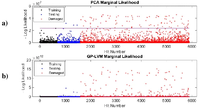
Figure 3 - Negative log marginal likelihood for both a) PPCA and b) GP-LVM, evaluated for training (black) and testing (blue) points from AE hits of undamaged bearing as well as data points from a damaged baring (red). The horizontal lines mark the 99.9th _{percentile of the training data.}

a)

The general approach for performing fault detection using these models is to train them using a set of data from an undamaged bearing, test their generalisation performance using a different set of data still from an undamaged bearing, and finally test their ability to highlight defects from a damaged bearing. The measure of discordancy used here has been the model likelihoods for both PPCA and GP-LVM as described in Equations 6 and 7. Figure 3 shows the negative likelihood evaluated for both models using hit data extracted from the training set, the testing set, and damaged set.

Note that both training and testing sets contain hits extracted from 15 seconds worth of AE data, each. The damaged set contains 30 seconds worth of data. The threshold shown in Figure 3 represents the 99.9th percentile of the training data, and we define an outlier here as an exceedance of that threshold.

Discussion of Results

Note that the success or otherwise of these models is dictated largely by the features used to train them. In this study we have selected rather simple features extracted from the time domain of each hit. Significant domain knowledge has therefore been used in the hit extraction process simplifying the task of the density estimator. It would be desirable, and left as further work to investigate this approach using richer features. It is evident that a GP-LVM outperforms PPCA in detecting outliers on damaged data. However, it also has more false positives in the test data set. To put these results in greater context, one would expect for these tests 15 outlying points per second, as this is the roller pass rate over the defect. The GP-LVM is clearly detecting more. This could be over-fitting from the model, from genuine secondary AE bursts from the defect, or from defects away from the loaded zone. In the inner raceway bearing used for this test, there are two more seeded defects, significantly away from the loaded zone. These sometimes also generate AE responses.

It is likely that the GP-LVM is over-fitting in this case. One can observe in Figure 3 b) that the training points are very concentrated compared to the damaged data, for the case of GP-LVM. PPCA on the other hand would appear to have outliers within the training set. Investigating these by hand shows that the outliers within the PPCA training set are hits so close to each other that they have been extracted as a single hit. This is in fact, a genuine outlier. This highlights that although the GP-LVM is able to capture more complexity within the training set, in doing so it assigns a high density even to outliers.

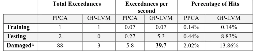
TABLE I – Comparative summary between PPCA and GP-LVM for outlier detection from AE data. Total Exceedances Exceedances per

second

Percentage of Hits

PPCA GP-LVM PPCA GP-LVM PPCA GP-LVM

Training 1 1 0.07 0.07 0.14% 0.14%

Testing 2 0 0.27 5.3 0.44% 8.83%

The result of this is the GP-LVM being sensitive to data from a damaged condition, but also being so sensitive that it marks many false positives. This is evident in Table I. Note carefully that the comparative results in Table I give a comparison using the 99.9th percentile of the training data as a threshold for an outlier. A sensitivity analysis of a threshold setting is outside the scope of this paper. However, it is worth noting that in the case of PPCA, which captures outliers within the training set, a much lower threshold is required for it to highlight all the damaged points. In the case of the GP-LVM, a threshold that is much further away from the training points is required since the training points are very tightly distributed while the outliers are separated significantly.

CONCLUSIONS

The GP-LVM was not originally designed to perform density estimation, it was designed as a tool for data exploration through dimensionality reduction. It has been shown here that it can successfully detect the AE bursts originating from a 5 𝜇𝑚 defect scribed on an inner raceway, by monitoring outside, on the bearing housing. A comparison between the density estimation from a GP-LVM and PPCA has been presented, showing that the GP-LVM can discriminate better between different sources of data compared with its linear counterpart - PPCA. Its sensitivity however also causes the GP-LVM to flag more false positives. There are several aspects that require further investigation, including sensitivity to threshold settings, features used, use of localisation, analysis of data collected from an in-service gearbox and extensions of these models that better model the density.

REFERENCES

1. J. R. Naumann, “Acoustic Emission Monitoring of Wind Turbine Bearings,” PhD Thesis, The University of Sheffield, 2015.

2. N. Lawrence, “Probabilistic non-linear Principal Component Analysis with Gaussian Process Latent Variable Models,” J. Mach. Learn. Res., vol. 6, pp. 1783–1816, 2005. 3. S. Roweis and Z. Ghahramani, “A unifying review of linear gaussian models.,” Neural

Comput., vol. 11, no. 2, pp. 305–345, 1999.

4. G. Manson, “Identifying damage sensitive, environment insensitive features for damage detection,” in 3rd International Conference on Identification in Engineering Systems, 2002. 5. M. J. Eaton, R. Pullin, J. J. Hensman, K. M. Holford, K. Worden, and S. L. Evans,

“Principal component analysis of acoustic emission signals from landing gear components: An aid to fatigue fracture detection,” Strain, vol. 47, no. SUPPL. 1, 2011.

6. K. Worden and C. R. Farrar, Structural Health Monitoring: A Machine Learning

Perspective. John Wiley & Sons, 2013.

7. C. E. Rasmussen and C. K. I. Williams, Gaussian processes for machine learning.

Cambridge, Massachusetts: The MIT Press, 2006.

8. H. Akaike, “A new look at the statistical model identification,” IEEE Trans. Automat.

Contr., vol. 19, no. 6, pp. 716–723, Dec. 1974.