Comment on “Examination of a Theoretical Model of Streaming Potential Coupling Coefficient”

(1)

Letter to the Editor

Comment on

(

Examination of a Theoretical Model of Streaming

Potential Coupling Coefficient

)

P. W. J. Glover

School of Earth and Environment, University of Leeds, Leeds LS2 9JT, UK

Correspondence should be addressed to P. W. J. Glover; [email protected]

Received 15 May 2015; Accepted 1 October 2015

Academic Editor: Rudolf A. Treumann

Copyright © 2015 P. W. J. Glover. This is an open access article distributed under the Creative Commons Attribution License, which permits unrestricted use, distribution, and reproduction in any medium, provided the original work is properly cited.

Recently, Luong and Sprik published an article that compared measurements that had been made on 20 samples of saturated rock with a number of empirical models and Glover et al.’s 2012 theoretical model for zeta potential and streaming potential coefficient. They found that none of the empirical models could reproduce the streaming potential coefficient measurements which had been made in the presence of low pore fluid salinities, and the theoretical method could only do so if a constant zeta potential was invoked. This contribution in the form of a comment (i) indicates at least three possible errors in modelling that contribute to the mismatch between the theoretical model and the data at low salinities and (ii) carries out individual modelling on all of samples of Luong and Sprik’s 2014 dataset, showing that Glover et al.’s 2012 theoretical model matches the data well when the zeta potential is allowed to vary and good match can only be obtained with a constant zeta potential if an unrealistic value of zeta potential offset is used.

1. Introduction

Recently, Luong and Sprik [1] published an examination of Glover et al.’s theoretical approach to zeta potential and streaming potential modelling of porous media [2, 3]. Luong and Sprik [1] recognized that although the comparison of the model with data in Glover et al. [3] was carried out with a large database which was extracted from the literature and which, at the time, was believed to represent a large portion of available data, there were problems with the test data. The problems included lack of reliable knowledge with regard to the pore fluid salinities, pH, and temperatures at which the experiments were carried out, as well as lack of the microstructural parameters for each sample. Microstructural rock parameters are necessary in order to carry out modeling for individual rock samples rather than generic rock types.

We have also recognized the same limitations in the published data and have set out independently to generate a high quality database in order to resolve the deficiency. The new approach to measurement which we developed was published in Walker et al. [4], and we now have 1253 measurements in our database.

Luong and Sprik [1] have followed the same approach. They have carried out high quality measurements on 20 rock

samples over a restricted salinity range (136 measurements). They compared their data with the available empirical models [5–8] for streaming potential coefficient. They also imple-mented Glover et al.’s [3] theoretical model for individual rock samples using the cementation exponent, formation factor, and permeability to characterize the rock microstructure. In this process, they effectively use the fluid permeability as a proxy for the rock’s modal grain size. Their conclusion was that none of the empirical models could account for the low salinity behaviour of the streaming potential coefficient, and neither could Glover et al.’s [3] model if the zeta potential was calculated with the approach of Revil et al. [9]. They repeated the model restricting the zeta potential to be constant following the assumption of All`egre et al. [10], whence they found that Glover et al.’s [3] model fitted the data well over the whole salinity range.

We have carried out theoretical modelling of Luong and Sprik’s [1] data and come to different conclusions. In particular, Glover et al.’s [3] theory models Luong and Sprik’s [1] data well at all salinities and with variable zeta potential within the limitations that we only know the limits of pore fluid pH under which the measurements were made.

This comment restricts itself to (i) making the results of our implementation of the modelling of Luong and Sprik’s [1]

(2)

Actual pore fluid concentration (mol/L)

Streaming potential coefficient (V/Pa)

1.E − 05 1.E − 04

1.E − 05 1.E − 03 1.E − 01 1.E − 06

1.E − 07

1.E − 08

1.E − 09

N = 7 pH= 6.7

pKMe= 7.5

pK(−)= 8 Γo= 10sites/nm2 dpore= 250 𝜇m

dgrain= 62.9 𝜇m

m = 1.983 𝜙 = 0.485 F = 4.2 Σcond= 6 ×10−8_S 𝜁o= −0.015V

DP50

RGPZ, variable zeta

RGPZ, zeta= −15mV

Exact solution, variable zeta

Exact solution, zeta= −15mV

Luong and Sprik [1], variable zeta

Luong and Sprik [1], zeta= −15mV

(a)

Actual pore fluid concentration (mol/L)

1.E − 05 1.E − 04

1.E − 05 1.E − 03 1.E − 01 1.E − 06

1.E − 07

1.E − 08

1.E − 09

N = 7 pH= 6.7

pKMe= 7.5

pK(−)= 8 Γo= 10sites/nm2 dpore= 250 𝜇m

dgrain= 62.9 𝜇m

m = 1.983 𝜙 = 0.485 F = 4.2 Σcond= 6 ×10−8_S 𝜁o= −0.045V

DP50

RGPZ, variable zeta

RGPZ, zeta= −45mV

Exact solution, variable zeta

Exact solution, zeta= −45mV

Luong and Sprik [1], variable zeta

Luong and Sprik [1], zeta= −45mV

[image:2.600.78.515.68.306.2]

(b)

Figure 1: A comparison of the three equations for modelling streaming potential coefficient using a variable zeta potential calculated with Revil et al.’s [9] approach (solid lines) and constraining the zeta potential to a constant value equal to (a)−15 mV (dashed lines) and (b)−45 mV (dashed lines), pH = 6.77. Protonic surface conductionΣprot

𝑠 = 6×10−8S.

data available in the literature and (ii) pointing out a number of reasons why it differs from that published by Luong and Sprik [1].

2. Modelling Difficulties

Luong and Sprik [1] retained most of the parameters used in Glover et al.’s [3] modelling in order to facilitate intercompar-ison. However, and significantly, they modified the equation for modelling the streaming potential coefficient. Glover et al. [3] had implemented the solution for the streaming potential coefficient using the equation

𝐶sp= 𝑑𝜀𝑓𝜀𝑜𝜁

𝜂_𝑓(𝑑𝜎_𝑓+ 4Σ_𝑠𝑚𝐹), (1)

which is an approximation of

𝐶sp= 𝑑𝜀𝑓𝜀𝑜𝜁

𝜂_𝑓(𝑑𝜎_𝑓+ 4Σ_𝑠𝑚 (𝐹 − 1)) (2)

for𝐹 ≫ 1. In these equations,𝐶spis the streaming potential

pressure coefficient relative to pore fluid pressure, in V/Pa [11],𝜂_𝑓is the dynamic viscosity of the pore fluid (in Pa⋅s),

𝜀_𝑓is the relative dielectric permittivity of the pore fluid (no units),𝜀_𝑜is the dielectric permittivity of vacuum (in F/m),𝜁 is the zeta potential (in V),𝑑is the modal grain size of the rock (in m),Σ_𝑠 is the specific surface conductivity (surface conductance, in S),𝜎_𝑓is the electrical conductivity of the pore fluid (in S/m), and𝐹is the formation factor (no units).

We will refer to (2) as the exact solution and (1) as the RGPZ solution. In these equations, the streaming potential coefficient depends upon a group of pore fluid properties

(𝜂_𝑓,𝜀_𝑓, and𝜎_𝑓), two interfacial properties(𝜁, Σ_𝑠), and two properties describing the microstructure of the rock (𝑑and

𝐹).

Luong and Sprik [1], however, considered that the modal grain diameter of the rock was not convenient, opting to rewrite (1) in terms of fluid permeability according to

𝐶sp= 𝜀𝑓𝜀𝑜𝜁

𝜂_𝑓(𝜎_𝑓+ 2 (Σ_𝑠/√8𝐹𝑘_𝑜)), (3)

where 𝑘_𝑜 is the steady-state fluid permeability of the rock. They do not provide a derivation or published reference for this equation.

There are three aspects of Luong and Sprik’s [1] modelling that are of concern, each of which is discussed in one of the following subsections.

2.1. Modelling Equations. The first is that we could not

generate (3) from either (1) or (2) using accepted relationships between 𝑑 and the characteristic pore size scale length Λ defined by Johnson et al. [12] and betweenΛand the steady-state permeability [13] or by using the RGPZ equation [14] or by invoking the well-known relationship𝑘_𝑜 = Λ2/2𝐹in the basic Helmholtz-Smoluchowski relationship [11]. In all cases, we obtain (3) but with the number 4 replacing 2 in the second term of the denominator.

(3)

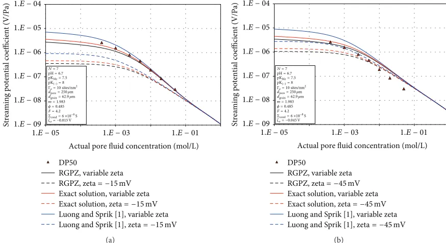
the modal pore diameter and used the Theta Transformation [15] to calculate the modal grain size. Hence, we have an independent value of grain diameter for use in (1) and (2). Both figures are for a pH of 6.7, which is the same as that used by Luong and Sprik [1]. The left-hand panel (Figure 1(a)) shows the models with zeta potential offset of−15 mV, which we find fits the data best and is consistent with values used by other authors. The right-hand panel (Figure 1(b)) shows the models with zeta potential offset of−45 mV, which is that used by Luong and Sprik [1] and is unrealistically high. Between them, these two diagrams incorporate all of the parameter values used by Luong and Sprik [1] and can hence be used to draw direct conclusions about the effectiveness of Luong and Sprik’s [1] implementations of the streaming potential coefficient modelling.

The solid lines in both parts of Figure 1 show the mod-els implemented with a variable zeta potential calculated according to the model of Revil et al. [9] as implemented by Glover et al. [3]. In the case of zeta potential offset of−15 mV, the RGPZ and Exact models with variable zeta potential perform well across the whole range of salinities represented by experimental data, with the Exact model marginally better. There is a little difference between the RGPZ and the Exact models, while Luong and Sprik’s [1] equation overestimates the streaming potential coefficient. It should be noted that if we carry out modelling with Luong and Sprik’s [1] equation replacing “2” with a “4,” the results are indistinguishable from the results given by the Exact model. Consequently, we detect an error in the equation that Luong and Sprik [1] used in their modelling that leads to overestimations of modelled streaming potential coefficient which are larger at low salinities. In the case of the zeta potential offset taking the higher value of−45 mV that was used by Luong and Sprik [1], all models overestimate the streaming potential coefficient at high salinities. This is because the true zeta potential in this range is lower in magnitude than−45 mV.

The dashed lines in Figure 1 show all three implemen-tations, but with a constant zeta potential of −15 mV in Figure 1(a) and a constant zeta potential of −45 mV in Figure 1(b). It is clear that none of the models perform well over the entire salinity range if the constant zeta potential is restricted to−15 mV (Figure 1(a)) with the modelled curves significantly underestimating the streaming potential coef-ficient in all cases. If we use−45 mV, which was that used by Luong and Sprik [1], we get higher values of constant zeta potential that are approximately consistent with the experimental data, but the models do not fit the data well. There are an underestimation of the streaming potential coefficient at low salinities and an overestimation at high salinities. This arises because the imposed constant−45 mV zeta potential is lower than the true zeta potential at low salinities and higher than the true zeta potential at the high salinities. This is primary evidence that a variable zeta potential is required to model the data. Consequently, it seems that the variable zeta potential predicted by Revil et al. [9] and supported by theory is required to model streaming potential coefficient.

Luong and Sprik [1] have used an erroneous model which overestimates the streaming potential coefficient when used

with a variable zeta potential as the full implementation of Glover et al.’s [3] approach requires. Consequently, they have restricted the zeta potential to remain constant and have compensated for the underestimation inherent in this approach by imposing a higher constant zeta potential which allows the lowest salinity experimental data to be modelled but overestimates the high salinity data, as shown by the blue dashed line in Figure 1(b). If they had used a variable zeta potential, their equation would produce modelled curves that would be accurate for high salinities but would be overestimated at low salinities, resulting in the effect of the microstructure on the modelled streaming potential coefficient being half of what it should be (solid blue line in Figure 1(a)).

The conclusions are clear: (i) Luong and Sprik’s [1] equation is in error. (ii) The error leads to overestimations at low salinities but does not affect high salinities. (iii) The use of a variable zeta potential is required to model the data. (iv) The use of a constant zeta potential of−45 mV compensates for the lack of a variable zeta potential, resulting in Luong and Sprik’s [1] model approaching the experimental streaming potential coefficient magnitudes, but not leading to good fit to them. (v) The implementation of the full model of Glover et al. [3] with variable zeta potential and a reasonable value of zeta potential offset provides the best fit to the experimental data across the entire range of salinities.

2.2. Fluid pH. The second concern is that while Luong and

Sprik [1] refer to their measurements being made with pore fluid pH between pH 6 and pH 7.7, no measurements of pH have been given for the individual sample data used in the paper by Luong and Sprik [1] and there is no indication of whether these pH values are for fully equilibrated or stock pore fluid solutions. It has been suspected for some time that the zeta potential and streaming potential coefficient are sensitive to pore fluid pH [2, 9] and this was confirmed in recent work [4]. The pH dependence of the zeta potential is particularly strong. The consequence of not having the pH of the pore fluids measured and reported is that streaming potential coefficient modelling cannot be carried out on individual samples because we do not know the pH from which the model curve can be calculated (Luong and Sprik [1] carried out their modelling at the representativead hoc

value of pH 6.7). In fact, in the absence of pH measurements for individual samples, we can only compare the data against curves representing the range of behaviours representing the pH values encountered during the measurements, and note that pH has an effect on both the zeta potential and the streaming potential coefficient which is greater at lower salinities than at high salinities.

2.3. Fluid Salinity. The third aspect of concern is that the

(4)

control of temperature. Consequently, most researchers do the best they can; then they measure the conductivity and pH of the resulting solutions for use in data presentation and modelling, so far, so pragmatically good. The problem comes when the solutions are passed through the core sample and become equilibrated with it. Geochemical interactions occur between the rock matrix and the pore fluid that are associated with dissolution and precipitation. These change the salinity, composition, and pH of the pore fluid. Walker et al. [4] found that there was a significant increase in the salinity of low salinity pore solutions (up to an order of magnitude) which makes it effectively impossible to make measurements with ultralow salinity pore fluids that are in equilibrium with a rock sample, while some reductions in pore fluid salinity could also occur at very high pore fluid salinities, this time due to precipitation.

The implications of this for making accurate experimental determinations are that not only must the pore fluid be passed through the rock sample until equilibration occurs before making any electrical conductivity or electrokinetic measure-ments on a saturated rock, but the electrical conductivity and pH of the fluids leaving the rock at the time measurement should be measured and taken as the state of the pore fluid that goes with the electrical or electrokinetic measurement.

Luong and Sprik [1] mention that the pore fluid has been equilibrated with the samples. We assume that the fluid pH values were also equilibrated in this process. Luong and Sprik [1] also mention that the resulting equilibrated pore fluid salinities were retained for zeta potential calculations. We also assume that the equilibrated pH values were also used in their zeta potential calculations. However, the final data is given in Table 2 in their paper and shown in the figures plotted against the stock solution salinities, which are now irrelevant.

In the case of Luong and Sprik’s [1] data, we are left wondering whether the salinity quoted for the data in Table 2 in their paper is valid for the measurement. If we take their lowest salinity stock solution (0.4 mmol/dm3) and their correlation between salinity, 𝐶_𝑓, and electrical conductivity,𝜎_𝑓 (𝜎_𝑓 = 9.5𝐶_𝑓− 0.0085), we obtain a pore fluid electrical conductivity of 1.23×10−2S/m. Walker et al. [4] found (Figure 4 in their paper) that a stock solution of this electrical conductivity would be increased by between 15% and 30% after equilibration with silica-based rocks. The larger of these two increases represents an increase of salinity from 0.4 mmol/dm3to 0.802 mmol/dm3, again using Luong and Sprik’s [1] relationship between pore fluid salinity and electrical conductivity. This represents an error on the salinity of the pore fluid of 100%. The error could be considerably larger in a carbonate rock or a rock with significant carbonate cement because dissolution and precipitation reactions are much more significant. Consequently, any modelled stream-ing potential coefficient curve that is calculated usstream-ing a stock solution salinity or its equivalent electrical conductivity would be significantly overestimated, with the degree of overestimation increasing as lower salinity pore fluids are used.

In summary, there are at least three sources of possible error, all of which might affect the modelled zeta potential

and streaming potential coefficient curves disproportionately at the low salinities where Luong and Sprik [1] observed that their data was not in agreement with the theoretical model.

3. Theoretical Modelling of Luong and

Sprik’s Data

We have carried out theoretical modelling of the zeta poten-tial and the streaming potenpoten-tial coefficient for the samples measured by Luong and Sprik [1] using our implementation of Glover et al.’s model [2, 3]. The modelling has been carried out on a sample by sample basis in order to fully account for differences in the microstructures of different samples.

For the sake of ease of comparison, most of the modelling parameters that we have used in this work are the same as those used by Luong and Sprik [1], who in turn took most of their modelling parameters from Glover et al. [3]. The sole exception is that we, as Luong and Sprik [1], have chosen to let the protonic surface conductance vary and obtain different values from them. This constancy of basic interfa-cial geochemistry parameters implies that (i) slightly better agreements with the experimental data might be possible and (ii) the modelling is only truly valid for silica-based rocks and will not be as good for carbonates or silica-based rocks that contain significant carbonate cement. Consequently, we would not expect the modelling of Luong and Sprik [1] samples EST, IND01 in that paper, to be modelled well by Glover et al.’s [3] approach unless further appropriate interfacial geochemistry modifications were made to the model.

The implementation of the model is the same as in Glover et al. [3], calculating the zeta potential from the approach used in Revil and Glover [16, 17] and Revil et al. [9] and then using (2) to calculate the streaming potential coefficient. Since Luong and Sprik [1] do not give the modal grain size for the rocks they have measured, we have calculated it from their permeability using the equation

𝑑grain= √4𝑎𝑚2_{𝐹 (𝐹 − 1)}2_𝑘

𝑜. (4)

This equation can be derived from the RGPZ permeability prediction equation [14] that includes 𝐹3 term. However, the RGPZ equation is an approximation of a more general equation [13] that is valid only if 𝐹 ≫ 1, which is clearly not the case for some of Luong and Sprik’s [1] samples (e.g., sample DP217, where𝐹 = 4.5). Consequently, (4) replaces

𝐹3_{term from the RGPZ equation with}_{𝐹(𝐹 − 1)}2_{to ensure}

validity for all of the rock samples for which we have data. Equation (4) can also be derived from the relationships𝑘_𝑜 =

Λ2/2𝐹andΛ = 𝑑grain/2𝑚(𝐹 − 1)with𝑎 = 2, whereas the

RGPZ equation is usually used with𝑎 = 8/3.

(5)

Model pH 6 Model pH 6.5 Model pH 7

Model pH 7.5 Model pH 8 BereaUS3

Reported pore fluid concentration (mol/L)

1.E − 05

1.E − 05 1.E − 03 1.E − 01 1.E + 01 1.E − 06

1.E − 07

1.E − 08

1.E − 09

1.E − 10

N = 7

pH=variable

pKMe= 7.5

pK(−)= 8

Γo= 10sites/nm2

dpore= 3.15 𝜇m

dgrain= 60.9 𝜇m

m = 1.59 𝜙 = 0.148 F = 21

Σcond= 8 ×10−8_S

𝜁o= −0.015V

(a)

DP46i Model pH 6

Model pH 6.5 Model pH 7

1.E − 05

1.E − 05 1.E − 03 1.E − 01 1.E + 01 1.E − 06

1.E − 07

1.E − 08

1.E − 09

1.E − 10

N = 7

pH=variable

pKMe= 7.5

pK(−)= 8

Γo= 10sites/nm2

m = 2.11 𝜙 = 0.48 F = 4.7

Σcond= 4 ×10−8_S

𝜁o= −0.015V

dpore= 35 𝜇m

dgrain= 102 𝜇m

(b)

DP50 Model pH 6

1.E − 05

1.E − 05 1.E − 03 1.E − 01 1.E + 01 1.E − 06

1.E − 07

1.E − 08

1.E − 09

1.E − 10

N = 7

T = ?∘_C

pHexpt= ?

pKMe= 7.5

pK(−)= 8

Γo= 10sites/nm

2

d = 200 𝜇m m = 1.72 𝜙 = 0.211 F = 14.5

Σcond= 1 ×10−7_S

𝜁o= −0.015V

(c)

BEN7 Model pH 6

1.E − 05

1.E − 05 1.E − 03 1.E − 01 1.E + 01 1.E − 06

1.E − 07

1.E − 08

1.E − 09

1.E − 10

N = 7

pH=variable

pKMe= 7.5

pK(−)= 8

Γo= 10sites/nm2

dpore= 19.11 𝜇m

dgrain= 234 𝜇m

m = 1.68 𝜙 = 0.222 F = 12.6

Σcond= 2 ×10−8_S

𝜁o= −0.015V

(d)

EST Model pH 6

1.E − 05

1.E − 05 1.E − 03 1.E − 01 1.E + 01 1.E − 06

1.E − 07

1.E − 08

1.E − 09

1.E − 10

N = 7

pH=variable

pKMe= 7.5

pK(−)= 8

Γo= 10sites/nm2

dpore= 7.032 𝜇m

dgrain= 69.5 𝜇m

m = 1.902 𝜙 = 0.315 F = 9

Σcond= 1 ×10−7_S

𝜁o= −0.015V

(e)

IND01 Model pH 6

1.E − 05

1.E − 05 1.E − 03 1.E − 01 1.E + 01 1.E − 06

1.E − 07

1.E − 08

1.E − 09

1.E − 10

N = 7

pH=variable

pKMe= 7.5

pK₍₋₎= 8

Γo= 10sites/nm2

dpore= 8.57 𝜇m

dgrain= 341 𝜇m

m = 2.15 𝜙 = 0.20 F = 32

Σcond= 1 ×10−7_S

𝜁o= −0.015V

[image:5.600.76.525.65.702.2]

(f)

Figure 2: Streaming potential coefficient modelling using (2) for six samples from Luong and Sprik’s [1] data as a function of pore fluid

salinity and pH together with the corresponding experimental measurements. (a) BereaUS3,Σprot

𝑠 = 8×10−8S; (b) DP46i,Σprot𝑠 = 4×10−8S;

(6)

−0.2

−0.15

−0.1

−0.05

0

Z

et

a p

o

te

n

tial (V)

Model pH 7.5 Model pH 8 Reported pore fluid concentration (mol/L)

1.E − 05 1.E − 03 1.E − 01 1.E + 01

(a)

−0.2

−0.15

−0.1

−0.05

0

Z

et

a p

o

te

n

tial (V)

1.E − 05 1.E − 03 1.E − 01 1.E + 01

(b)

−0.2

−0.15

−0.1

−0.05

0

Z

et

a p

o

te

n

tial (V)

1.E − 05 1.E − 03 1.E − 01 1.E + 01

(c)

−0.2

−0.15

−0.1

−0.05

0

Z

et

a p

o

te

n

tial (V)

1.E − 05 1.E − 03 1.E − 01 1.E + 01

(d)

−0.2

−0.15

−0.1

−0.05

0

Z

et

a p

o

te

n

tial (V)

1.E − 05 1.E − 03 1.E − 01 1.E + 01

(e)

−0.2

−0.15

−0.1

−0.05

0

Z

et

a p

o

te

n

tial (V)

1.E − 05 1.E − 03 1.E − 01 1.E + 01

[image:6.600.86.513.68.691.2]

(f)

(7)

which represent the worst agreement (DP50 and BEN7), and two examples which represent the typical behaviour (EST and IND01). Figure 3 shows the corresponding zeta poten-tials which were calculated during the streaming potential coefficient modelling, also as a function of salinity from 10−5mol/dm3 to 10 mol/dm3and for five values of pH from pH 6 to pH 8. This figure differs between samples only due to the use of different protonic surface conductances because the interfacial geochemistry parameters (e.g., various binding and dissociation constants as well as surface site densities and shear plane distance; see Glover et al. [3]) have all been kept constant.

In interpreting Figures 2 and 3, we should bear in mind the three difficulties mentioned in the last section. The first difficulty, the problem with the modification to the streaming potential coefficient equation, has been resolved by the use of our existing implementation of the model and using a grain size given by (4). We could have used the Theta Transformation [15] to provide the grain size from the quoted pore sizes as in Figure 1 but chose to obtain our grain sizes from the permeability measurements for all samples in order to ensure that the same process was carried out for all samples.

The second difficulty, which lies in the ambiguity of the pore fluid pH, is overcome by modelling curves for 5 values of pore fluid pH between pH 6 and pH 8, between which we are told by Luong and Sprik [1] that the pore fluid pH lies.

The last difficulty, that of not knowing the true salinity of the pore fluid in the samples at the time of the electrokinetic measurements, can only be overcome while interpreting Figures 2 and 3. The probable case that all of the low salinity data given by Luong and Sprik [1] are valid for somewhat higher pore fluid salinities operating within the rock than the stock solution salinities at which they are plotted causes the low salinity data in every part of Figures 2 and 3 to appear to droop towards lower pH curves, with the effect being greater at lower salinities. Consequently, we hypothesise that these points are misplotted because of the ambiguity in their pore fluid salinity. The salinity of the fluid in the rock at the time of the measurement would have been higher than that of the stock solution by about 100% at the lowest salinities used in the experimental measurements according to Walker et al. [4], so these data points need to be shifted to the right, whereupon they often conform to a single pH curve from the model.

Overall, there is extremely good agreement between the experimental data and the model curves in all cases. The worst cases occur for carbonates and for those which contain significant carbonate cement as expected. Carbonates not only require a different set of parameters for calculating the zeta potential; some of the equations that have been used to handle the permeability, pore size, and grain size deter-minations are valid only for clastic rocks, having difficulty when applied to carbonates. The agreement for almost all of the 20 samples extends across the whole salinity range and incorporates a variable zeta potential. Reference to Figure 3 shows that although the zeta potential varies as a function of pore fluid salinity and pH very much, there is little difference

between the curves in Figure 3. This is because all the samples share similar properties as a result of their silica-based matrix, and consequently their fundamental electrochemical parameters are the same or similar.

4. Conclusions

Luong and Sprik’s [1] implementation of Glover et al.’s [3] theoretical model for calculating the zeta potential and streaming potential of silica-based rocks suffers from a number of difficulties, (i) in one of the equations that have been used, (ii) in the control of the pH, and (iii) in the knowledge of the salinity of the pore fluid. When those difficulties are either resolved or corrected or their effects are understood, Glover et al.’s [3] theoretical model produces a good agreement of the streaming potential coefficient with Luong and Sprik’s [1] experimental data at all salinities providing the zeta potential to vary with pore fluid salinity and pH according to the approach developed by Revil et al. [9]. It is possible to obtain reasonable fit to the experimental data with a constant zeta potential, but this requires an unrealistically high value of the zeta potential offset to achieve it. Furthermore, our current electrochemical understanding of the electrical interface between the pore fluid and the rock matrix (e.g., [11]), which defines the zeta potential, provides irrefutable theoretical (e.g., [9, 13, 16, 17]) and experimental (e.g., [4, 6, 7, 18]) evidence that the zeta potential in porous materials varies with both salinity and pH. Consequently, the conclusions reached by Luong and Sprik [1] are misleading, and the constant zeta potential as a function of pore fluid salinity that was proposed [8, 10] is oversimplification of the true salinity and pH dependencies of the zeta potential.

Conflict of Interests

The author confirms that no conflict of interests exists in the submission of this comment.

Acknowledgments

The author would like to thank the coauthors of previous papers contributing to this comment, particularly Emilie Walker, Matthew Jackson, and Nicholas D´ery.

References

[1] D. T. Luong and R. Sprik, “Examination of a theoretical model of

streaming potential coupling coefficient,”International Journal

of Geophysics, vol. 2014, Article ID 471819, 12 pages, 2014. [2] P. W. J. Glover and N. D´ery, “Streaming potential coupling

coefficient of quartz glass bead packs: dependence on grain diameter, pore size, and pore throat radius,”Geophysics, vol. 75, no. 6, pp. F225–F241, 2010.

[3] P. W. J. Glover, E. Walker, and M. D. Jackson, “Streaming-potential coefficient of reservoir rock: a theoretical model,”

Geophysics, vol. 77, no. 2, pp. D17–D43, 2012.

(8)

fractured rocks,”Journal of Geophysical Research: Solid Earth, vol. 119, no. 2, pp. 957–970, 2014.

[5] S. R. Pride and F. D. Morgan, “Electrokinetic dissipation

induced by seismic waves,”Geophysics, vol. 56, no. 7, pp. 914–

925, 1991.

[6] J. Vinogradov, M. Z. Jaafar, and M. D. Jackson, “Measurement of streaming potential coupling coefficient in sandstones saturated

with natural and artificial brines at high salinity,”Journal of

Geophysical Research: Solid Earth, vol. 115, no. 12, 2010. [7] M. Z. Jaafar, J. Vinogradov, and M. D. Jackson, “Measurement of

streaming potential coupling coefficient in sandstones saturated with high salinity NaCl brine,”Geophysical Research Letters, vol. 36, no. 21, Article ID L21306, 2009.

[8] L. Jouniaux and T. Ishido, “Electrokinetics in earth sciences: a tutorial,”International Journal of Geophysics, vol. 2012, Article ID 286107, 16 pages, 2012.

[9] A. Revil, P. A. Pezard, and P. W. J. Glover, “Streaming potential

in porous media. I. Theory of the zeta potential,”Journal of

Geophysical Research: Solid Earth, vol. 104, no. 9, Article ID 1999JB900089, pp. 20021–20031, 1999.

[10] V. All`egre, L. Jouniaux, F. Lehmann, and P. Sailhac, “Streaming potential dependence on water-content in Fontainebleau sand,”

Geophysical Journal International, vol. 182, no. 3, pp. 1248–1266, 2010.

[11] P. Glover, “Geophysical properties of the near surface earth: electrical properties,” inTreatise on Geophysics, G. Schubert and D. Bercovici, Eds., vol. 11, pp. 89–137, Elsevier, Oxford, UK, 2nd edition, 2015.

[12] D. L. Johnson, J. Koplik, and L. M. Schwartz, “New pore-size

parameter characterizing transport in porous media,”Physical

Review Letters, vol. 57, no. 20, pp. 2564–2567, 1986.

[13] A. Revil and L. M. Cathles III, “Permeability of shaly sands,”

Water Resources Research, vol. 35, no. 3, pp. 651–662, 1999. [14] P. W. J. Glover, I. Zadjali, and K. A. Frew, “Permeability

prediction from MICP and NMR data using an electrokinetic approach,”Geophysics, vol. 71, no. 4, pp. F49–F60, 2006. [15] P. W. J. Glover and E. Walker, “Grain-size to effective pore-size

transformation derived from electrokinetic theory,”Geophysics,

vol. 74, no. 1, pp. E17–E29, 2009.

[16] A. Revil and P. W. J. Glover, “Theory of ionic-surface electrical

conduction in porous media,”Physical Review B, vol. 55, no. 3,

pp. 1757–1773, 1997.

[17] A. Revil and P. W. J. Glover, “Nature of surface electrical

con-ductivity in natural sands, sandstones, and clays,”Geophysical

Research Letters, vol. 25, no. 5, pp. 691–694, 1998.

[18] J. Vinogradov and M. D. Jackson, “Zeta potential in intact

nat-ural sandstones at elevated temperature,”Geophysical Research

(9)

Submit your manuscripts at

http://www.hindawi.com

Hindawi Publishing Corporation

http://www.hindawi.com Volume 2014

Climatology

Journal of

Ecology

Earthquakes

Journal of Hindawi Publishing Corporation

Hindawi Publishing Corporation http://www.hindawi.com

Applied &

Environmental

Soil Science

Volume 2014

Mining

International Journal of

Geophysics

Oceanography

International Journal of

Journal of Computational Environmental Sciences

Journal of

Petroleum Engineering

Geochemistry

Journal of

Atmospheric Sciences

Oceanography

Advances in

Mineralogy

Meteorology

Advances in

The Scientific

World Journal

Paleontology Journal Hindawi Publishing Corporation

Scientifica

Geological ResearchJournal of