Addressing Missing Data in Viral Genetic Linkage Analysis Through Multiple Imputation and Subsampling-Based Likelihood Optimization

Addressing Missing Data in Viral

Genetic Linkage Analysis Through

Multiple Imputation and

Subsampling-Based Likelihood Optimization

The Harvard community has made this

article openly available.

Please share

how

this access benefits you. Your story matters

Citation

Erion, Gabriel Gandhi. 2015. Addressing Missing Data in Viral

Genetic Linkage Analysis Through Multiple Imputation and

Subsampling-Based Likelihood Optimization. Bachelor's thesis,

Harvard College.

Citable link

http://nrs.harvard.edu/urn-3:HUL.InstRepos:17417574

Terms of Use

This article was downloaded from Harvard University’s DASH

repository, and is made available under the terms and conditions

applicable to Other Posted Material, as set forth at http://

Addressing Missing Data in Viral Genetic Linkage

Analysis Through Multiple Imputation and

Subsampling-Based Likelihood Optimization

A thesis submitted by

Gabriel Erion

To

Applied Mathematics

in partial fulfillment of the honors requirements

for the degree of

Bachelor of Arts

Harvard College

Cambridge, Massachusetts

Abstract

This thesis addresses the intersection of two important areas in epidemiology and statistics: genetic linkage analysis and missing data methods, respectively. Genetic linkage analysis is a promising method in viral epidemiology which involves learning about transmission patterns by studying clusters of similar gene sequences. For example, similar sequences found in a pair of geographically distinct communities may imply disease transmission between the two locations. However, this analysis is sensitive to missing data, which can introduce substantial bias. This thesis presents a multiple-imputation approach which corrects for much, though not all, of the bias in genetic linkage analysis. It also introduces a novel resampling-based approach that generates a weighted distribution of complete datasets and is even more effective than imputation for reducing bias. This work highlights the importance of missing data in genetic linkage studies and presents ways to provide more accurate epidemiological information by correcting for missing data. The new resampling-based approach presented in this paper is also general enough to be applied to many types of missing-data problems involving complex datasets; such broader applications are a promising avenue for future research.1

1_{Code used in this thesis is available on Github athttps://github.com/gabeerion/thesis_2015}

Acknowledgements

There are many people without whom this thesis could not have been written. First, I must extend my most heartfelt gratitude to my advisor, Professor Victor De Gruttola. Over the past three years, working in his research group has immeasurably expanded both my skills and my confidence as a statistical researcher, and showed me the enduring joy of applying rigorous quantitative analysis to challenging problems. I would also like to thank Professor Joe Blitzstein not only for introducing me to statistics and teaching me many techniques which would be invaluable in this thesis, but also for discussing early drafts with me.

Many other members of my research group have provided guidance for which I am deeply grateful. Dr. Ravi Goyal has answered countless questions about Markov Chain Monte Carlo methods, and also provided my first introduction to network analysis. Dr. Vlad Novitsky guided me through the world of phylogenetic analysis and was incredibly knowledgeable about HIV biology and the challenges of working with large genetic datasets.

I would also like to thank the friends who selflessly took the time to read and provide comments on early versions of this thesis. Casey Fleeter, Robert Francis, Jake Freyer, Leo Guttmann, Dianna Hu, Ola Topczewska, and Paul Wei all read drafts with extraordinary care and thoughtfulness. They are what Patrick Rothfuss called “the kind of friends everyone wishes for but no one deserves.”

Finally, and most importantly, a lifetime’s worth of thanks to my parents, RL and Saila Erion. My gratitude for the curiosity and passion for learning you inspired in me is second only to my gratitude for twenty-one years of unconditional love and support. I love you and cannot thank you enough.

Contents

1 Introduction 13

1.1 HIV in Botswana . . . 14

1.2 Viral Genetic Linkage Analysis . . . 15

1.2.1 VGL Method . . . 16

1.2.2 Application . . . 19

1.3 Impact of Missing Data on Genetic Linkage Analysis . . . 22

1.4 Review of Missing Data Methods . . . 23

1.4.1 Mechanisms of Missingness . . . 25

1.4.2 Methods for Addressing Missing Data . . . 26

1.5 Overview of Following Sections . . . 28

2 Multiple Imputation 29 2.1 Framework . . . 29

2.2 Multiple Imputation Method . . . 32

2.3 Evaluation . . . 34

2.4 Discussion . . . 37

3 Subsampling-Based Likelihood Optimization 41 3.1 Background . . . 41

3.2 Subsampling Method . . . 43

3.3 Closed-Form Calculation . . . 45

3.4 Evaluation . . . 49

3.4.1 Data . . . 49

3.4.2 Results . . . 49

4 Distribution-Based Approaches 53 4.1 A Full Distribution over Missing Data . . . 53

4.2 MCMC Sampling . . . 55

4.2.1 Overview of MCMC . . . 55

4.2.2 Proposal Methods . . . 57

4.2.3 Target Distribution . . . 59

4.3 Sampling by Distribution Optimization . . . 62

5 Discussion and Conclusions 65 5.1 Broader applications . . . 65

5.2 When to Use These Methods . . . 67

5.3 Caveats . . . 68

List of Figures

1.1 Graph corresponding to adjacency matrixM. . . 20 1.2 Plots of randomly generated points in 2-dimensional space, withx, y∈(0,1). 24 1.3 Histograms of the distribution of the distance from each random point in

2-dimensional space to its nearest neighbor for 128, 64, 32, 16, and 8 points. . 24 2.1 A representative deletion of 100 sequences substantially reduces clustering,

and imputation recovers much of this bias. . . 37 2.2 Distributions of minimum distances from original dataset of 371 sequences,

datasets with 100 sequences deleted, and datasets with 200 sequences deleted. 39 3.1 Diagram of a process for assessing quality of an imputed dataset. . . 44 3.2 Convergence of subsampledcsubestimates to exactly calculated value. . . 48

3.3 Minimizing|csub−cobs|favors datasets that minimize error in estimating c. . 51

List of Tables

2.1 Mean clustering statistics c and coverage proportions for full data (ctrue), observed data (cobs), and multiple imputation estimate (cimp),

over 1,000 simulations . . . 36 4.1 Mean Squared Error and Coverage of Optimization and Imputation

Methods . . . 63

Chapter 1

Introduction

Inference in the presence of missing data is one of the most difficult problems in statistics, and a substantial body of literature addresses methods for performing such inference. One arena in which missing data becomes uniquely challenging is in the epidemiology of infec-tious disease. A powerful new idea in this field is that genetic sequence data of infecinfec-tious microorganisms can be used to reconstruct information about the transmission networks along which diseases spread. This Viral Genetic Linkage (VGL) analysis relies on the idea that genetically similar microbes that infect different patients are likely to share a common evolutionary ancestor, implying that the infected patients are part of the same transmis-sion chain. Epidemiologists have documented the ability of VGL to infer properties such as transmission rate, degree of disease exchange between communities, and even drug resis-tance. However, the fact that VGL relies not only on the distribution of individual genotype data but also on relationships between pairs of data points makes it particularly sensitive to missing data.

In this thesis, I present several increasingly sophisticated methods to correct for miss-ingness in genetic sequence data, and demonstrate the ability of these methods to improve VGL analysis and epidemiological inference using a viral genetic dataset collected from HIV patients in Mochudi, Botswana. The first approach, multiple imputation, involves building a biological model to simulate missing gene sequence data. The second approach uses a re-sampling procedure to search for datasets that “fill in” missing gene sequences and maximize the likelihood of the incomplete dataset we did observe. Finally, I explore methods that generate a distribution of complete datasets, with higher-likelihood datasets given greater weight.

This thesis makes several contributions to the statistical and epidemiological literature. First, it demonstrates the bias that missing data can introduce in epidemiological studies of infectious disease, particularly VGL analysis. Second, it introduces a collection of novel, well-founded methods for general statistical inference in the presence of missing data. Fi-nally, it demonstrates the effectiveness of these methods in the context of genetic sequence data and epidemiological inference by substantially reducing the bias in VGL analyses of HIV. My hope is that the availability of such methods will improve the tools policymakers and public health practitioners use in infectious disease policy and practice.1

1.1

HIV in Botswana

Botswana is one of the countries hardest-hit by the HIV epidemic and also one of the first African countries to implement a strong national response through testing and treatment. Historically, Botswana has had one of the highest HIV prevalences of any country; a 2011 study found prevalence to be 30.4% among women aged 15–49 [1]. Studies credit HIV/AIDS

1_{All code written for this thesis is publicly available on Github at https://github.com/gabeerion/}

1.2. VIRAL GENETIC LINKAGE ANALYSIS 15 with a staggering 28-year decrease in life expectancy in Botswana between 1990 and 2006 [2]. One of the first major interventions undertaken by the government was a prevention of mother-to-child transmission (PMTCT) program begun between 1999 and 2001. Provision of free antiretroviral therapy (ART) began in 2002 and has been scaled nationwide [2]. The government of Botswana estimates that 67% of the total HIV-infected population is receiving antiretroviral therapy [1]. The government is continuing to work to increase access to ART, particularly among pregnant women, difficult-to-reach or stigmatized populations such as men who have sex with men (MSM), and individuals who have high risk for infection or for transmitting the disease.

The data used in this study was collected from Mochudi, Botswana, a community of over 44,000 people in southeastern Botswana. Since 2011, a pilot study in Mochudi has performed community-wide household surveys, provided HIV testing, and offered lab testing for viral load and CD4 count to HIV positive participants. The pilot study was itself a precursor to a larger planned study that would extend these services to 30 communities across Botswana and provide treatment for all patients with viral loads above 10,000 copies/mL [3]. The dataset analyzed in Chapter 2 represents 371 HIV subtype C gene sequences collected by the end of the first phase of the study in spring 2012. The data used in Chapters 3 and 4 consists of 1248 sequences collected between the beginning of the study in 2011 and summer 2014. The sequences are all from the V1C5 region of theenv gene, aggregated as a multiple sequence alignment.

1.2

Viral Genetic Linkage Analysis

epidemiological conclusions: for example, if many sequences in a community are genetically similar, the disease in question may be spreading quickly without time to accumulate mu-tations. If similar genetic sequences are found in geographically distinct communities, this may imply transmission between the two, and so on.

1.2.1

VGL Method

More formally, we can represent sequence data as an n×m matrix, where there are n

patients in the population and a gene sequence ofmsites is collected from each patient. We consider only datasets consisting of aligned sequences, which is reasonable considering that VGL is based on assessments of sequence similarity. Thus we might have an alignment A

like the following:

A=            

A T G C C . . .

A T G T G . . .

..

. ... ... ... ... . ..

A T G C G . . .

                                  

| {z }

msites

nsequences

1.2. VIRAL GENETIC LINKAGE ANALYSIS 17 collected from one patient. It can be written as

si =

A T G C G . . .

The core step in VGL analysis is to form clusters of genetically similar sequences, which will form the basis for epidemiological inference. There are many ways these clusters can be defined. Phylogenetic methods that involve building a tree are a natural way to define clusters; branch length and preservation of proximity across bootstraps can be used to assign sequences to clusters [4–6]. Genetic distances between sequences can also be used to create clusters. One method is simple hierarchical clustering; another approach involves building a graph where nodes represent sequences and edges represent pairs of sequences that are separated by a distance below a given threshold [6]. Clusters can then be constructed from cliques or connected components in the graph. Previous work with VGL analysis in our group has focused on this last approach: to construct clusters we build a distance matrix and consider as clusters all connected components in the induced graph. It is worth noting that clustering methods such ask-means are not considered in this paper. Whilek-means is a simple and effective clustering method, it involves pre-specifying the number of clusters to be found. Since this number is itself useful information, it seems preferable to use biological knowledge about the genetic sequences in question to specify a reasonable genetic distance cutoff and see how many clusters naturally emerge.

For the purposes of assessing sequence similarity in the population, we construct a pair-wise distance matrix between all sequences. Let the distance matrixDbe constructed such that Dij = d(si, sj) according to some distance metric between sequences. For example,

if we use the Hamming distance (defined as d(a, b) = Pk

i=1I(ai 6=bi) where aand b are

sequencessi andsj feature different nucleotides. Hamming distance is a very simple

met-ric, and does not account for differential rates of mutation between different nucleotides or different frequencies of mutation at different sites in a sequence. Evolutionary biologists have developed many more complex metrics of genetic distance, which use known mutation frequencies to estimate the evolutionary time required to mutate one sequence into another. This study uses Hamming distance for simplicity; however, it’s important to note that one advantage of VGL is that it can incorporate arbitrary distance metrics. A simple and ef-ficient or complex and biologically realistic model can be used as desired, so long as it is possible to construct a pairwise distance matrix.

For example, if we have the very small alignment

A=                

A T G C C G G

A T G T C G G

A T G C C G G

A T G T G G G

A T G A A G G

               

Then the resulting distance matrix is

D=                

0 1 0 2 2 1 0 1 1 2 0 1 0 2 2 2 1 2 0 2 2 2 2 2 0

1.2. VIRAL GENETIC LINKAGE ANALYSIS 19 To form clusters, we need to choose a genetic threshold distance t below which we consider sequences similar enough to share a cluster. In general, one would like this distance to be chosen with some prior knowledge about expected genetic diversity of the infectious agent. If the maximum possible genetic distance is dmax, sequences si and sj cluster if

d(si, sj)≤ tdmax. In the case of Hamming distance, dmax = m because no sequence can

differ from another at more thanmsites. For illustration, if we choose the arbitrary threshold

t= 0.25 so that the threshold distance istm= (0.25)(7) = 1.75, then two sequencessi and

sj are considered “linked” ifd(si, sj)≤tm= 1.75. The adjacency matrix for the resulting

graph, which will also be called the “clustering matrix”, has entry i, j equal to 1 if si and

sj are linked and 0 otherwise. Formally,Mij =I(Dij≤tm)I(i6=j) =I(Dij ≤1)I(i6=j).

M =                

0 1 1 0 0 1 0 1 1 0 1 1 0 0 0 0 1 0 0 0 0 0 0 0 0

               

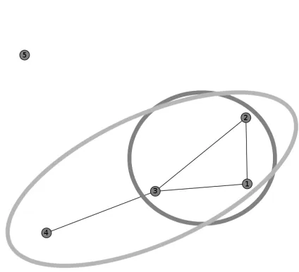
Note that we remove self-loops for clarity; a “cluster of one” is considered trivial. The graph itself can be seen in Figure 1.1. If a cluster is defined as a clique, sequences (rows) 1, 2, and 3 form a cluster. If a cluster is defined as a connected component, as in this paper, sequences 1, 2, 3, and 4 form a cluster.

1.2.2

Application

Figure 1.1: Graph corresponding to adjacency matrixM. If a cluster is defined as a clique, sequences 1, 2, and 3 form a cluster (dark grey). If a cluster is defined as a connected component, as in this paper, se-quences 1, 2, 3, and 4 form a cluster (light grey).

[4, 7–9]. The literature surveyed here focuses primarily on HIV, both because it has been the focus of many efforts to leverage genetic information in public health and because studies focusing on HIV are most closely related to the work in this thesis.

Several studies use the size of sequence clusters to infer the number of neighbors of each patient in the transmission network; this approach also allows for direct estimation of the basic reproduction numberR0 [10–12].2 Further, [12] shows that the distribution of

cluster sizes can be used to estimate prevalence of HIV as well asR0. When temporal data

is available, the time between infections in a cluster can be used to estimate transmission rates (the number of transmissions per unit time) [13,14]. In addition, [14] incorporates data on infection stages to determine that transmission rates vary over the course of infection.

Viral genetic linkage analysis becomes especially useful, however, when clustering be-tween and within communities and populations is analyzed. For example, [13] compares transmission rates estimated from epidemics occurring within heterosexual transmission networks to those estimated from MSM (men who have sex with men) networks, and finds that epidemics in heterosexual populations exhibit lower transmission rates. There is

par-2_{The basic reproduction numberR}

1.2. VIRAL GENETIC LINKAGE ANALYSIS 21 ticularly strong public health interest in understanding which clusters new infections tend to fall into, with the hope that targeting these clusters for treatment can reduce the rate of new infections. Several papers have noted that new infections tend to cluster with other recent infections [4, 15]. Drug resistance is another characteristic of interest, and sequences featuring resistance mutations also tend to cluster together [7]. Epidemics in heterosexual, MSM, and IDU (intravenuous drug user) populations feature different avenues of transmis-sion and different epidemiological characteristics; viral genetic linkage analysis has shown that sequences from any one of these subpopulations tend to cluster together [16]. However, clusters often contain both heterosexual and IDU patients, indicating that while the MSM epidemic is relatively isolated, cross-transmission occurs between the heterosexual and IDU epidemics. At a broader level, VGL has been used to assess transmission dynamics between communities. One study replicated the finding that heterosexual and MSM epidemics do not intermix, but did find clusters spanning multiple countries and noted evidence of trans-mission between populations in Nairobi and coastal Kenya [17]. A similar study using all publicly available HIV-1 polymerase sequences built a global map of viral genetic linkage between all countries and found multiple transmission clusters that crossed borders [18].

to individuals with high risk scores predicted significantly reduced HIV transmission across the whole network.

1.3

Impact of Missing Data on Genetic Linkage

Analysis

The clusters studied in Viral Genetic Linkage Analysis become challenging to work with when data is missing because they depends on interactions between data points. Because of these dependencies, even data that is missing uniformly at random can induce bias in estimates. In particular, suppose that the property of interest, which we will call c, is defined as the proportion of sequences in the dataset that fall into any cluster. That is, how many sequences out of the total are close enough to some other sequence to fall below the genetic distance threshold? Because sequences and the distances between them are analyzed in a very high-dimensional space (for example, 1,000 dimensions define a 1,000-nucleotide sequence), it is hard to visualize how deletions affect the distances between sequences. However, the same principles apply to points in smaller spaces, like 2-dimensional Euclidean space, as well. Later chapters will demonstrate an empirically observed bias incas sequences are deleted from HIV datasets (See Figures 2.1 and 2.2, as well as Table 2.1); this section will illustrate how missingness leads to biases in the distribution of distances by examining more easily visualized data in 2-dimensional space.

Figure 1.2 shows 128 points drawn at random from the unit square, that is withx, y∈

1.4. REVIEW OF MISSING DATA METHODS 23 the proportion of points falling into a cluster tends to decrease (0.95, 0.86, 0.69, 0.63, 0.75). The threshold distance here is a Euclidean distance of 0.1. Note that though these are clear trends they are not monotonic. Occasionally, by random chance, the deleted points will be those which are far away from the rest; these deletions will decrease the average distance between points. Figure 1.3 shows histograms of the distance of each point to its nearest neighbor, which demonstrate that the distribution of minimum distances between points spreads out to larger and larger values as more points are deleted. In particular, the more points are deleted, the less probability mass remains on the left side of the threshold distance.

The overall proportion of clustering for a gene sequence alignment is calculated in the same way and can be interpreted as the probability mass of sequences that fall left of the threshold genetic distance, so it is vulnerable to the same mechanism of bias. As more sequences are deleted from the dataset, the distribution of distances between sequences becomes skewed toward larger values and less clusters emerge. Previous work has found that, in HIV testing studies, up to 40% of data is missing (minimum response rates are 60% among men and 70% among women) [20]. This illustrates the need for methods which can address the biases induced by missing sequence data.

1.4

Review of Missing Data Methods

Figure 1.2: Plots of randomly generated points in 2-dimensional space, with x, y∈ (0,1). This visualization shows that as points are deleted, the average distance between points increases. When distance metrics are used to define clusters, fewer clusters will be observed as points are deleted, even if deletions are uniformly random. The bias introduced in VGL sequence analysis is exactly the same but in a much higher-dimensional space.

1.4. REVIEW OF MISSING DATA METHODS 25 have developed for addressing missing data, from heuristics to rigorously justified alorithms.3 Mechanisms of missingness and common methods for addressing missing data are discussed below.

1.4.1

Mechanisms of Missingness

It is possible to distinguish between three types of missing data, as discussed in [22]. Methods for addressing missingness will vary based on the mechanism by which data went missing.

• Missing Completely at Random (MCAR): In these cases, the probability that a particular data point from the full dataset goes missing is distributed uniformly, so that all points are equally likely to be missing. This is the least challenging scenario because ignoring the missing data still yields a dataset that is a representative, random sample from the population. However, as noted in the previous section, MCAR still results in bias when the statistic of interest is a function of the distances between data points in some space. Thus many methods that are generally assumed to work under MCAR will not always be suitable for VGL analysis.

• Missing at Random (MAR): When data are missing at random, the probability that a data point is missing depends on observed characteristics of the data but not on unobserved characteristics. For example, it is possible to categorize HIV patients into multiple demographic groups. If sequences from patients in different demographic groups have different probabilities of going missing, but all patients within a given group are equally likely to be missing, the data are MAR. This setting is more chal-lenging because ignoring missing data doesnot result in a representative random sam-ple. However, knowledge of which data are most likely to be missing makes it possible

to adjust for the missing data by stratifying before performing inference, reweighting existing data points or simulating new data. This is the case that applies when we know how many sequences in each demographic group are missing, but not what the sequences are.

• Not Missing at Random (NMAR): Data are NMAR if missingness depends on unobserved characteristics of the missing data; for example, if whether a sequence goes missing depends on properties of the actual sequence. Addressing missingness in this framework is extremely challenging, and is impossible without specifying a model for the process by which data goes missing. In the context of HIV, sequences would be NMAR if missingness depended on the distance between a sequence and its nearest neighbor, which is impossible to estimate without knowing the missing sequence. Though the NMAR setting is not explicitly studied in this thesis, so long as a mechanism for missingness can be specified, the subsampling-based methods presented in Chapters 3 and 4 can incorporate this mechanism to address NMAR data.

1.4.2

Methods for Addressing Missing Data

• Complete case analysis simply refers to eliminating missing data from analysis (only studying complete cases). It has the advantage of being very simple, but is problematic because it fails in all but the MCAR scenario. Complete case analysis can also reduce power because the size of the dataset is reduced.

1.4. REVIEW OF MISSING DATA METHODS 27 will occur in all but MCAR settings), mean imputation will reinforce the wrong mean. Mean imputation is particularly problematic in the sequence analysis setting: the most natural implementation would be to replace all missing sequences with the consensus sequence.4 _{However, this causes particularly serious problems when properties of}

interest depend on genetic distance, as introducing many copies of the same consensus will result in a large number of zero genetic distances (in contrast, the datasets used here involve the variableenv gene and have no zero distances). Thus, in VGL studies, mean imputation may be worse than complete case analysis.

• Regression imputation uses a regression model to predict values of the missing data based on the observed data, then performs analysis on the “full” dataset. This method works very well in the MCAR setting, and is also effective in MAR if the variables that determine missingness are included in the regression. This method does tend to unrealistically reduce variance of the data by imputing data along the regression line; however, this problem can be overcome by adding noise to the imputed values (stochastic regression imputation). More importantly, in the context of VGL analysis, it is difficult to generate new sequences based on observed ones with a simple regression; more sophisticated models are required. In addition, stochastic regression imputation draws noise from the observed distribution of residuals, which may not give an accurate assessment of the variance of estimates for arbitrary properties of interest.

• Reweighting methods, in particular inverse probability weighting, weight data points that were more likely to go missing under the missingness model more highly in the analysis. Reweighting methods are a very popular way to handle missing data, but

some types of data cannot be reweighted in a straightforward manner. In particular, it is challenging to reweight genetic distance data between pairs of points. However, recent work in our research group has made progress on applying concepts from inverse probability weighting to sequence linkage analysis [23].

The techniques listed above do not constitute an exhaustive list; however, they do rep-resent some of the most common approaches to handling missing data. Many of them are difficult to apply to VGL analysis or will yield biased estimates of the properties we are interested in studying. For this reason, the first method we present will be a very powerful technique not yet mentioned: multiple imputation.

1.5

Overview of Following Sections

Chapter 2

Multiple Imputation

One of the most intuitive approaches to dealing with missing data is to build a random model that can be used to simulate additional data until the dataset is “complete.” Iterating this process multiple times to account for model variance and averaging across the results is known as multiple imputation, and is widely regarded as a gold standard technique for handling missing data. In this section, I demonstrate how a multiple imputation approach can reduce bias and improve estimates of variance in VGL analyses. Most of this section is based on work in my research group submitted for publication in [24].

2.1

Framework

Recall that we start with a matrix A representing a genetic sequence alignment of n se-quences and m sites. The rows of this alignment are a proper subset of the rows of an unobserved, “true” full dataset which we’ll call A∗. Let us rewritenasno, for the number

of observed sequences, and denote the number of missing (unobserved) sequences asnm, so

that the total number of sequences inA∗ isnt=no+nm. The goal is to use theno×m

alignmentAto estimate a set of new imputed alignments{A01...A0k}, each annt×m

align-ment. For a given A0

i, the first no rows should correspond exactly to A while the last nm

rows represent inferred sequences.

Suppose we are interested in estimating a property c of the true alignment A∗, and letf denote the function that calculates this property, so that c =f(A∗).1 _{Estimating c}

from the observed data, cobs = f(A) is the most obvious solution; we may even be able

to estimate the variance vobs = Var(c) of this estimate by bootstrapping [25].2 However,

this estimator is biased for most properties of interest (examples were shown in Section 1.3) and bootstraps may give incorrect variance estimates. In the multiple imputation framework, we use the imputed alignmentsA0_i to obtain a more accurate estimate ofc and its variance. In particular, we calculateCimp={c1imp...ckimp}={f(A01)...f(A0k)} as well as

Vimp={vimp1 ...vkimp}={Var(c1imp)...Var(ckimp)}. Then the multiple imputation estimate for

cis just the mean of Cimp:

cimp=

Pk

i=1c

i

imp

k

The variance estimate is calculated as in [26]:

vimp=

Pk

i=1v

i

imp

k +

k+ 1

m Var(Cimp)

In [26] the first term is referred to as the “within-imputation variance”, and represents the average variance of any individual estimate. The second term is the “between-imputation variance”, and represents the variance of the vector of all estimates taken together.

1_{In all work in this paper, alignmentsA, A}0_{, A}∗_{are matrices of characters or discrete integers representing}

those characters, and the properties cto be estimated are real numbers. While functions mapping, for example, from matrices to vectors or other objects are not considered in this paper, it is usually possible to incorporate them into this framework.

2.1. FRAMEWORK 31 The multiple imputation formulas given above allow for the estimation of arbitrary statistics and the construction of confidence intervals even when data is known to be missing, so long as it is possible to impute full datasets{A0₁...A0_k}.

The main remaining question is how to imputek datasets ofnt×m rows and columns

from the observed data. If all that is observed is theno×mmatrixA, we may not even know

nt. Not only are we unaware of the content of the missing rows, we do not even know how

many rows there are! It is essential to have some information about how much data is missing and what kind of data it is. The approach adopted here makes use of two additional kinds of information to begin the imputation process, both acquired from census data. First, HIV prevalence statistics can be used to calculate the expected number of HIV patients in a population. This number is used asnt, the observed number of sequences isno and

nm=nt−no. Second, demographic information can be used to place patients into categories

that provide more information about patterns of missingness. For example, if there are d

different demographic categories in the population, then each sequence can be assigned a number between 1 anddrepresenting which category it falls into. Thus, demographic data for the entire population can be represented as a vector T of length nt where each entry

is a patient’s demographic category. Given this information, we know both the number and type of missing sequences. For example, if there are two demographic categories of interest, prevalence data may tell us not only that there arenmmissing sequences but that

twice as many of these sequences fall into category 1 as into category 2. This allows us to construct a vector F of probabilities, with length d, where the ith entry represents the proportion of the population falling into category i. Thus, the available information for imputation consists of an alignmentA, a number of missing sequencesnm, and perhaps also

demographic proportions F. The next section will show how to use this information to simulate thenmmissing sequences.

2.2

Multiple Imputation Method

Given the information above, a model of evolutionary mutations can be used to impute the

nm missing genetic sequences. The key observation enabling imputation is that each

se-quence in the population has a nearest neighbor, as measured by genetic distance. In terms of the pairwise genetic distance matrixD, the nearest neighbor for sequence i is given by argmin_j(Dij).3 To impute a new sequence, two key assumptions are made: first, that the

sequence’s nearest neighbor is one of the observed sequences, and second, that the distance between the sequence and its nearest neighbor is represented in the observed distribution of pairwise distances. Under these assumptions, a new sequence can be generated by drawing a genetic distance from the observed distribution of pairwise distances, then copying an ex-isting sequence and mutating that sequence until it is the desired distance from the original. Throughout this process, it is assumed that the demographic information Tobs and F is

available; when no demographic information is available, the entire population is considered as one demographic group. In these cases,Tobs is a vector assigning every sequence to the

category 1, andF = (1). That is,F denotes that the entire population falls into the single available category.

Before imputing, we need to know how many sequences to impute. If no demographic information is available, the number of sequences to impute is simplynm. If demographic

information is available, we can calculate how many sequences should be imputed in each

2.2. MULTIPLE IMPUTATION METHOD 33 category in order to make the demographic proportions in the data equal toF; denote these numbers asFimp.4

The first step in the imputation process is building the distribution of pairwise distances to be drawn from. In particular, we want to sample a plausible distance between the imputed sequence and its nearest neighbor, so the desired distribution is built from the distance between each observed sequence and its nearest neighbor,N ={minj(Dij)|i∈no}. When

demographic traits are given, this additional information can be incorporated by building nearest-neighbor distributions for each pair of demographic groups. Nab={minj(Dij)|Ti=

a, Tj =b} is the distribution of nearest-neighbor distances from a sequence in groupato a

sequence in group b. BecauseNab and Nba are different distributions (i being j’s nearest

neighbor does not meanj isi’s nearest neighbor), this results in a total ofd2_{distributions,}

though the total number of nearest-neighbor distances is the same regardless of how many distributions these distances are partitioned into.

Next, a specific sequence is imputed. Its demographic category a is drawn from Fimp.

Next, the demographic categorybof its nearest neighbor needs to be chosen. We drawb∈ {1...d}with probability proportional to|Nab|. This guarantees that demographic categories

which are most frequently seen as nearest neighbors of sequences in category a are most likely to be chosen as nearest neighbors for the imputed sequence.5 _{A nearest-neighbor}

distancel is then drawn fromNab.

The new sequencesj is initialized as a copy of its nearest neighbor sequencesi, chosen

uniformly at random from the demographic category b. Mutations are then applied to sj

untild(sj, si) =l. In general, these mutations can be applied in very simple ways (such as

4_{If no demographic information is available, sequences will be imputed uniformly at random until there} arentsequences

making mutations to the sequence uniformly at random), or very sophisticated ones ( [27] presents software for simulating sequence evolution along a phylogeny). The method used here strikes a balance between simplicity and sophistication, and has the added benefit that it makes no prior assumptions about mutation frequencies, instead estimating these frequencies from the data. In particular, a nt× |Σ| matrix W is constructed where each

rowWe is a multinomial probability distribution over the characters found at sitee in the

observed alignment A. Sites are chosen one at a time for mutation; the probability of mutating sitee is proportional to 1−max(We). Thus sites that are highly conserved are

only rarely mutated while sites that are highly variable are mutated frequently. When a character at a specific site is mutated, the replacement character for that site is drawn as a weighted sample fromWe. This process is repeated untild(sj, si) =l.

The new sequence sj is added to the alignment, and the above steps are repeated to

impute new sequences until the alignment has nttotal rows, resulting in an alignmentA01.

Note that as the alignment grows in size, previously imputed sequences may be chosen as nearest-neighbor sequences to be copied and mutated. The process is repeated k times to yield k alignments of size nt×m. Estimation of alignment properties and variance is

performed as described above.

2.3

Evaluation

2.3. EVALUATION 35 of my research group’s work in [24], we evaluated the above method on HIV genetic data collected from Mochudi, Botswana.

The evaluation dataset consists ofnt= 371 HIV subtype C sequences collected from the

community survey in Mochudi, Botswana mentioned in Section 1.1. The overall percentage of the population which fell into a cluster was used as the estimated property of interest

c. Sets of 50, 100, and 200 sequences were repeatedly deleted from the full dataset: for each nm ∈ {50,100,200}, 100 different subsampled datasets of no = nt−nm sequences

were generated. In this study, the population was divided into demographic categories – young males, young females, old males, and old females. Females were deleted at a rate 10 times higher than that of males to demonstrate the effectiveness of the method when different population subgroups are missing at different rates. For each subsample, multiple imputation ofk= 10 datasets was performed 100 times to yield 100 estimates ofcas cimp

and variances of these estimates, vimp. Thus, for each number of deletions, it is possible

to compare 10,000 multiple imputation estimates to estimates resulting from the observed data over a random sample of possible deletions.

For each multiple imputation, we compared the clustering values c calculated from the full dataset to values calculated from only the observed (subsampled) data and to values calculated from a multiple imputation estimate. We also estimated coverage of 95% confi-dence intervals around the estimates from observed data and from multiple imputation – the proportion of times that a 95% confidence interval around an estimatecobsorcimpcontained

95%. In general, the closer the coverage is to 95% the more reliable the estimator. In gen-eral, the clustering statistic estimated only from observed data, cobs, is biased downwards.

Multiple imputation (cimp) substantially reduces bias (though does not eliminate it), and

improves coverage proportions. As more sequences are deleted, estimates from the observed data suffer from an increasing degree of bias. The multiple imputation estimate suffers from less bias, though as missingness becomes severe it does display downward bias as well. The full results, calculated for [24], are presented in Table 2.1 below.

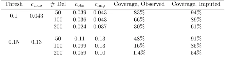
Table 2.1: Mean clustering statistics c and coverage proportions for full data (ctrue), observed data (cobs), and multiple imputation estimate (cimp), over 1,000

simulations

Thresh ctrue # Del cobs cimp Coverage, Observed Coverage, Imputed

50 0.039 0.043 83% 94% 0.1 0.043

100 0.036 0.043 66% 89% 200 0.024 0.037 30% 61%

50 0.11 0.13 48% 91%

0.15 0.13

100 0.099 0.13 16% 85% 200 0.059 0.10 1.4% 54%

Thresh indicates the minimum genetic distance (in proportion of total sequence length) below which two sequences were considered part of a cluster. The average clustering value estimated by multiple imputation is closer to the true value than that estimated with the observed data alone, and coverage proportions are also higher.

2.4. DISCUSSION 37

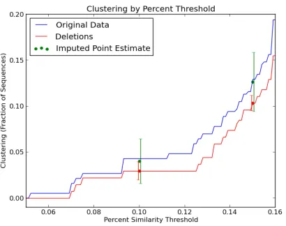
Figure 2.1: A representative dele-tion of 100 sequences substantially reduces clustering, and imputation recovers much of this bias. Also note that only confidence intervals around the imputed estimates include the true clustering value.

at the 0.1 and 0.15 genetic distance thresholds, the difference betweenc in the full dataset and the subset is equal to the median difference across 100 different subsamples.

First, calculations using only the dataset that underwent deletions are biased; clustering is substantially lower in the dataset that experienced deletions than in the original data. Second, calculations based on the dataset that experienced deletions underestimate the variance of c; note that the red bars indicating 95% confidence intervals for the value of

c using the dataset that experienced deletions do not include the true value. Estimates from multiple imputations are less biased and considerably closer to the true value ofc. In addition, these estimates exhibit larger variance and confidence intervals that include the true value ofc.

2.4

Discussion

One important reason is that the imputation method presented here imputes new sequences in a way that maintains the observed distribution of minimum genetic distances between sequences; however, this observed distribution itself is likely biased by deletions. Because the clusterng proportion is based on the distribution of minimum distances, preserving bias in this distribution will ensure some bias always remains in estimates ofc.

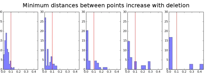
The bias in minimum distance distribution can be seen through simulation; in the figure below, subsets of 100 and 200 sequences were repeatedly deleted uniformly at random from the full dataset of 371 sequences. Minimum distances from 100 independent repetitions were pooled and the distributions compared at each number of deletions. Small but statistically significant increases in genetic distance are seen with each increase in the number of deleted sequences. Median genetic distances are 97.0 for the original data (n=371), 98.0 for datasets with 100 deletions (n=2710), and 101.0 for datasets with 200 deletions (n=1710). Differences between distributions were significant as follows:

• Original Data and 100 Deletions: p <0.05 (Mann-WhitneyU-test, U= 472856)

• Original Data and 200 Deletions: p <0.00001 (Mann-Whitney U-test,U = 267360)

• Original 100 Deletions and 200 Deletions: p <0.000001 (Mann-WhitneyU-test,U = 2086828.5)

(Note that power differs between tests because of different sample sizes).

2.4. DISCUSSION 39

Figure 2.2: Distri-butions of minimum distances from original dataset of 371 se-quences, datasets with 100 sequences deleted, and datasets with 200 sequences deleted. Visual inspection and Mann-Whitney U test confirm that the dis-tribution of genetic distances tends to increase a small but significant amount as more sequences are deleted.

Chapter 3

Subsampling-Based Likelihood

Optimization

3.1

Background

This chapter will attempt to address some of the main shortcomings of the multiple impu-tation framework. One concern about this framework is that it makes multiple assumptions that are difficult to justify. In particular, the random model used to impute new sequences by applying mutations is a drastic oversimplification of real biological evolution. Applying mutations independently at each site with probability proportional to their frequency in the observed data ignores correlations between mutations at different sites and assumes the ob-served data is a representative sample of mutation frequencies. Another example of a flawed assumption in multiple imputation is the method’s reliance on preserving the observed dis-tribution of minimum distances between sequences, though this disdis-tribution is biased as discussed at the end of the last chapter. It is of course possible to use many different models

to impute missing sequences, and more realistic models than the one presented in Chapter 2 certainly exist. However, it is unlikely that any model will perfectly replicate sequence evolution, so some biases will persist. Multiple imputation has no way to account for flaws in the imputation model; rather, it blindly averages results over multiple runs of the model. This accounts for the variance of estimates but ignores biases in the model. A second, re-lated concern is that multiple imputation treats all imputed datasets equally by taking an unweighted average over results from each imputation. Some imputed datasets will more accurately fill in missing sequences than others, but the multiple imputation framework has no way to prefer such “higher-quality” datasets.

Both of these concerns could be addressed in a straightforward way if the full datasetA∗

were known. Given a statistic of interestccalculated using the functionf and an imputed dataset A0, we can compare the values of c calculated from the full dataset and imputed dataset,c∗=f(A∗) andcimp=f(A0) respectively. DatasetsA0for which|cimp−c∗|is small

are less biased and should be preferred in the estimation process. Though this weighting process is simple, it is also impossible to use in practice becauseA∗ andc∗ are unknown. If we knewc∗, we would not have to estimate it at all!

In practice, estimation procedures have access only to the observed, incomplete dataset

Aand the statistic estimated from this datasetcobs =f(A). The only information available

about the full datasetA∗ is that, after undergoing deletion ofnmsequences, it gives rise to

the observed alignmentAand observed statisticcobs. Intuitively, we should prefer imputed

datasets which, when they undergo deletion ofnmsequences, yield observed statistics close

3.2. SUBSAMPLING METHOD 43

3.2

Subsampling Method

Given an imputed dataset A0 and full, unobserved dataset A∗, both consisteng of nt

se-quences, one way to assess how close A0 is to A∗ is to subsample no sequences fromA0 a

total of k different times, resulting in k incomplete datasets A1

sub...Aksub. Calculating the

statistic of interest on each of these incomplete datasets yieldskestimates ofc,c1

sub...cksub.

The average of these estimates, or

csub=

Pk

i=1c

i

sub

k

approximates the expected value ofc when estimated from any subsample ofno sequences

fromA0. DatasetsA0 for which|csub−cobs|is small are favorable because they are similar

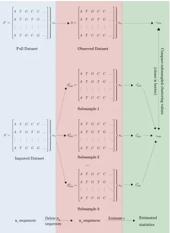
to A∗ in the one way we can observe: when they undergo deletions, they result in similar estimates of the statisticc. See Figure 3.1 for an illustration of this comparison process.

While it can be shown that imputed datasets that minimize|csub−cobs|produce more

ac-curate estimates ofc, the resampling procedure used to calculatecsubposes several problems.

First, repeated subsampling and calculation ofcfor each subsample can be computationally expensive. Second, it is unclear a priori how many subsamples are required to produce a stable estimate of the expected subsampled value ofc, orcsub. Fortunately, for the statistic

Figure 3.1: Diagram of a process for assessing quality of an imputed dataset. Both the imputed dataset and the complete data have the same number of sequences, but the complete dataset is unavailable for comparison. The imputed dataset is subsampled multiple times, resulting in many datasets of the same size as the observed data. The average estimate of

c, or csub across these datasets is compared to the observed value of c, or cobs. The more

3.3. CLOSED-FORM CALCULATION 45

3.3

Closed-Form Calculation

Consider an imputednt×m alignmentA0. Recall that the pairwise distance matrix, here

denotedD0, is constructed by measuring the genetic distance between all pairs of sequences; for distance metricd,D_ij0 =d(si, sj). Letdmax be the maximum possible genetic distance;

because we generally want to ignore sequences whose only neighbor is themselves, it is generally convenient to setd(si, si) =dmax. For some thresholdt∈(0,1), any two sequences

siandsj for whichD0ij≤tdmaxare considered “linked” and will be part of the same cluster.

The statistic of interestcis the proportion of sequences which are part of any cluster; that is, which are close enough to any other sequence to share a cluster with it. The clustering matrixM0is a binary matrix with entries defined as 1 if the distance between two sequences falls below the threshold and 0 otherwise: M_ij0 =I(Dij ≤tdmax)I(i6=j). The statisticc is

then simply the proportion of rows that contain a 1 at any point, or

c=

Pnt

i=1I(

Pnt

j=1Mij ≥1)

nt

This is simple to calculate with a single pass over the matrix M0_{. However, we want to}

calculate not justcbut csub, which is the expected value ofccalculated on a subsample of

no sequences fromA0. In other words, ifc were calculated using each of the _nnt

o

possible subsampled alignments, its mean value would be csub. It is possible to approximate csub

by randomly generating subsamples of A0, but exactly calculating csub this way is wildly

impractical. For the 371-sequence sample considered here, a typical subsample where 100 sequences are missing yields 371₂₇₁possible subsamples, or roughly 3.73×1092.

each subsample. However, by using linearity of expectationcsub can indeed be calculated

in closed form. LetAbe a matrix-valued random variable which is ano×mmatrix drawn

uniformly at random from all subsamples ofnosequences fromA0. Denote the corresponding

pairwise distance matrix asD and the clustering matrix asM. Then:

csub=E

Pno

i=1I(

Pno

j=1Mij ≥1)

no

!

By linearity, we can move the expectation inside the sum:

csub=

Pno

i=1E

I(Pno

j=1Mij ≥1)

no

=

Pno

i=1P(

Pno

j=1Mij≥1)

no

(3.1)

This expression still depends on the specific form of the clustering matrixM corresponding to the subsample A, however. We would like it to depend only on M0, the full clustering matrix. We focus on the termPPno

j=1Mij ≥1

: P   no X j=1

Mij≥1



=

nt

X

i0₌₁

P   no X j=1

Mij ≥1|Ai =A0i0 

P(Ai=A0i0)

3.3. CLOSED-FORM CALCULATION 47 complement of the probability that no neighbors are sampled:

P   no X j=1

Mij≥1|Ai=A0i0 

= 1−P 



no

X

j=1

Mij= 0|Ai=A0i0 

= 1− _n

m

nt

Pntj=1M 0

i0j

(3.2) Because sampling happens uniformly at random, each sequence is chosen to be part of the subsample independently of the other sequences. Thus the probability that no neighbors of sequencei0 are sampled is the probability of any individual sequence not being sampled

nm

nt

raised to the power of the number of neighbors sequence i0 has. The numerator on the RHS of (3.1) can now be written as

no X i=1 P   no X j=1

Mij ≥1

 = no X i=1 nt X

i0₌₁

1−

_n

m

nt

Pntj=1M 0

i0j!

P(Ai=Ai0)

All sequences in the alignmentA0 are equally likely to end up as a given sequenceAi in A,

soP(Ai =Ai0) = 1

nt. Upon making this substitution, the expression no longer depends on

i, so we can simplify:

no

X

i=1

nt

X

i0₌₁

1−

_n

m

nt

Pntj=1M 0

i0j!

P(Ai=Ai0) =

nt

X

i0₌₁

no nt 1− _n m nt

Pntj=1M 0

i0j!

The full equation forcsub from the RHS of (3.1) can now be written as:

csub=

Pnt

i=1

no

nt

1−nm

nt

Pntj=1M 0 ij no = nt X i=1 1 nt 1− _n m nt

Pntj=1M 0

ij!

(3.3)

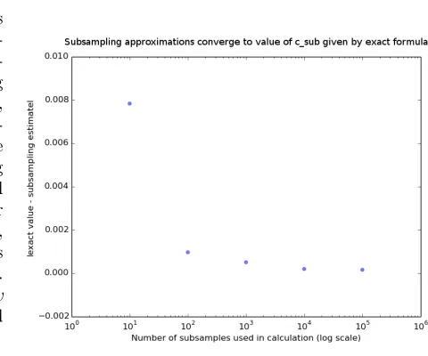
Figure 3.2: Convergence of sub-sampled csub estimates to

ex-actly calculated value. X-axis represents number of subsam-ples used to estimate csub

(es-timated subsampled clustering value using Hamming distance, as used throughout this pa-per). Y-axis represents absolute difference between subsampling estimate and exactly calculated value for csub. As the number

of subsamples used increases, the estimate of csub converges

to the exactly calculated value. Dataset is 200 HIV-C env

gp120 V1C5 sequences collected from Mochudi, Botswana.

combinatorial explosion of terms involved in calculating csub by subsampling. Figure 3.2

below demonstrates that values of csub calculated using subsampling converge to the value

calculated with the exact formula. The key property that allows for closed-form calcula-tion ofcsub is that d(si, sj) is independent of other sequences, that is, of all sk for which

k 6= i, k 6= j. This property is what lets us relate Mij and Mi0_j in equation (3.2); the

probability that sequenceiin Ahas at least one neighbor depends entirely on whether one of its neighbors in the original alignment A0 _{was sampled. It’s worth noting that not all}

distance metrics have the property thatd(si, sj) depends only onsiandsj; in particular, for

distances calculated using a phylogeny,d(si, sj) depends on all other sequences in the

3.4. EVALUATION 49

3.4

Evaluation

3.4.1

Data

Because the work in this chapter and those succeeding it occurred at a later date than the work presented in Chapter 2, a new dataset was available for analysis. All subsequent re-sults are based on a dataset consisting of a 1248-sequence, 1797-nucleotide alignment of the V1C5 region of HIV-Cenv gp120 sequences collected from patients in Mochudi, Botswana. Because the methods presented later in this thesis are, in general, more computationally intensive, subsets of the full dataset are often chosen. As there are many possible sub-sets, many (generally 100) subsamples are considered and the subsample with the median clustering proportioncis chosen.

3.4.2

Results

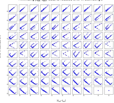
As can be seen in Figure 3.3, minimizing |csub−cobs| does indeed reduce absolute error

in estimatingc over 100 different 30-sequence subsamples of a 50-sequence dataset (all se-quences from the dataset discussed immediately above). The median correlation between

|csub−cobs| and absolute error in estimatingc isr = 0.38. The heterogeneity of behavior

under subsampling is surprising, however. A substantial number of subsampled datasets ex-hibit behavior we would expect of rare, pathological cases: for these subsamples,|csub−cobs|

points; others have two offset positively correlated lines and a single set of negatively corre-lated points. This implies that, while the behavior of sequence datasets when subsampled is complex, this behavior can be decomposed into combinations of a few simple behaviors. Future studies into the structure of these correlations could yield valuable information. In addition, that the correlation is somewhat weaker than expected supports the expansion of this method by comparing not just one subsampled statistic but many. If weak positive correlations hold for all of these statistics, favoring datasets that minimize|csub−cobs|for

many statisticscshould minimize error even further in estimating all properties of interest. These results also have implications for how we should use information about csub to

inform missing data analysis. Given that there is a correlation between |csub−cobs| and

estimation error, one approach to dealing with missing data would be to impute a dataset and iteratively optimize it to minimize |csub−cobs|. This is the best dataset to analyze

in the sense that it behaves most similarly to the original data in the ways that we can observe (that is, its behavior under subsampling). Though the results in this section imply that datasets generated using such a method would be more likely to be accurate than an arbitrarily chosen imputed dataset, the wide range of correlations observed in Figure 3.3 imply that it will still often yield inaccurate estimates, because in a substantial minority of subsamples |csub−cobs| exhibits a negative correlation with error. In these cases, the

optimized dataset is being optimized in the wrong direction! While a single dataset which minimizes|csub−cobs| is an improvement over a random imputed dataset, we can still do

better. Generating adistributionof datasets, each optimized to different values of|csub−cobs|

3.4. EVALUATION 51

Figure 3.3: Minimizing |csub−cobs| favors datasets that minimize error in estimating c.

This set of simulations started with a dataset of 50 sequences × 1797 nucleotides; out of 100 such subsamples of the full dataset, the one with median clustering valuecwas chosen for representativeness. One hundred different subsamples of 30 sequences were taken, and 100 imputations of 20 new sequences performed on each. For each subsampled dataset, a scatter plot is shown of the absolute difference between the subsampled clustering value

csub for the imputed dataset and the clustering value observed in the subsampled dataset

of 30 sequencescobs (x-axis) and the absolute error in the imputed dataset’s estimate of c

(plots sorted by decreasing correlation coefficient). Most datasets demonstrate a positive correlation between |csub −cobs| and error in the estimate of c; for some datasets this

correlation is smaller and in some cases it is negative. These exceptions are expected in our model; some subsets of the data are outliers in terms of their values ofcobs and are not

representative of the typical behavior of the orignal dataset under subsampling. Overall, the relationship between |csub−cobs| and estimation error is usually positive, with mean

Chapter 4

Distribution-Based Approaches

The resampling-based approach presented in the last section demonstrates reduced bias and error in recovering clustering estimates, in that imputed alignmentsA0 that minimize

|csub−cobs|are more likely to produce accurate estimates ofc. However, it is not immediately clear how to incorporate this knowledge into a method that not only provides estimates of

cbut also allows for construction of accurate confidence intervals around the estimate. The approaches presented below seek to recover a distribution over the true value of c that incorporates as much information as possible from the observed data.

4.1

A Full Distribution over Missing Data

It is relatively clear that, because datasets with lower values of|csub−cobs|tend to produce

more accurate estimates, they should be weighted more highly. However, it is difficult to justify any particular weighting scheme over any other. For example, w= _|c 1

sub−cobs| (used

above) andw= 1− |csub−cobs|both prefer datasets with smaller differences between the

The arbitrary nature of the weighting function underlies a fundamental question: can we generate a distribution over all possible datasets that fill in missing data representing our belief that a given dataset represents the “truth”?

The problem is not at all trivial; first, it requires exploring a massive space. In the examples in Chapter 2, the full dataset consists of 371 sequences and a deletion of 100 is considered, so the goal is to use 271 observed sequences to impute 100 more. Considered as nucleotides, these 100 sequences consist of 1647 bases; each can be one of five characters (A,C,T,G, or gap). The total number of possible ways to fill in these sequences is the number of ways to generate one hundred 1647-character strings from an alphabet of 5 characters, or 5100×1647≈10427096_{(for comparison, there are only 10}81_{atoms in the observable universe).}

Second, the problem requires constructing a reasonable way to weight each of these possible datasets so that it is possible to make quantitative measurements of how much more likely one dataset is than another. Finally, a method for drawing datasets according to this metric from a huge sample space is required to obtain actual numerical results.

The overall process can be split into two steps: formulating a desired distribution over all possible datasets, and approximating this distribution by sampling. As in Chapter 3, our only source of information about the full distribution is the subsample we observe and the statistic estimated from it,cobs. Thus, rather than specifying the relative frequencies with

which each dataset should be drawn, we can specify the relative frequencies with which datasets with given values of csub should be drawn. The idea that datasets minimizing |csub−cobs|result in the most accurate estimates implies our distribution should place the

most weight on these datasets. In addition, by bootstrapping the columns of the observed alignment A, we can estimate the variance of the statisticcobs and require that the target

distribu-4.2. MCMC SAMPLING 55 tion overcsub that determines what proportion of the desired sample has various expected

clustering values after subsampling. We will call this proxy distribution P; the goal is to draw datasets so that the values ofcsubcorresponding to each dataset fit the distributionP.

This collection of datasets represents our belief about the likely ways to fill in the missing sequence data. Given such a collection of datasets, it is possible to calculate an estimate of

c, by averaging over ci =f(A0i) for each datasetA0i in the distribution. Similarly, the

vari-ance of the estimate is the varivari-ance of theci. Higher order moments can also be estimated

because the datasetsA0_iare samples from the distribution over all possible datasets. The challenge that remains is to draw samples from this distribution. The following sections present two sampling methods for this task. The first, a Markov Chain Monte Carlo based approach presented in Section 4.2, was ultimately unsuccessful. The second, based on optimizing a distribution of datasets for similarity to the distribution P, was successfully implemented and is presented in Section 4.3.

4.2

MCMC Sampling

4.2.1

Overview of MCMC

The first step in implementing Metropolis-Hastings is to initialize the first state of the Markov chain. In this case, the states being considered are datasets, so the first state will ideally be a candidate full dataset of relatively high probability. The multiple imputation method discussed in Chapter 2 provides a convenient method for generating a plausible initial state; simply impute a singlent×mdatasetA01as the first step of the chain.

To generate the rest of the chain, we require a rule for stepping from state to state which will cause the chain to converge to the target distributionT. Given a stateA0_i, the key idea of Metropolis-Hastings is to propose a new state A0prop. The next state in the chain state

A0

i+1 will be chosen with some probability fromA0i and A0prop, and the process will begin

again. Theacceptance probability ais the probability thatA0_propwill become the next state

A0_i+1; if not, we setA0_i+1=A0_i and continue. The value ofais defined as

a= min

_T(A0

prop)

T(A0

i)

Q(A0

prop→A0i)

Q(A0

i→A0prop)

,1

(4.1)

whereT(A0_i) andT(A0_prop) represent the likelihoods of the current state and proposed new state in the target distribution and only need be determined up to a constant of proportion-ality. That is,T(A0

i) andT(A0prop) do not need to be exactly determined so long as the ratio

T(A0 prop)

T(A0

i)

is correct. Q(A0_i→A0_prop) represents the probability of proposing stateAprop from

4.2. MCMC SAMPLING 57

4.2.2

Proposal Methods

Given some state A0_i which is a full dataset ofnt sequences that fills in the missing data,

there are many ways to propose a new stateA0_prop. The only absolute requirements are that the proposal method alters only the nmmissing sequences, not the no observed sequences

(as these are known to represent sequences actually present in the population), and that the likelihood of steps between states can be calculated up to a proportionality constant (so that it is possible to calculate the term Q(A

0 prop→A

0

i)

Q(A0

i→A0prop)

). Three proposal methods are easily available based on previous work and the techniques presented in this thesis:

• Uniform Proposal: Simply make a certain number of random mutations for each proposal. Pick k sites to mutate, uniformly distributed across the nm unobserved

sequences and m sites in each sequence, and mutate the character currently present at each site to another character uniformly at random.

• Transition Matrix: Pick k sites to mutate as in the uniform proposal. However, instead of mutating the characters at these sites uniformly at random, use a transition matrixH that allows for differential rates of mutation between different characters, so thatHij represents the probability of mutation from characterito characterj. Many

such transition matrices have been constructed from empirical data for phylogenetic analysis, and can readily be applied in this proposal method. This approach has the advantage of making mutations that are more frequently observed in real sequences. One important advantage of these first two methods is that they can be used to generate

symmetric proposals; that is, proposals in which Q(A0

prop →A0i) =Q(A0i → A0prop). Such

methods are advantageous because there is no need to explicitly calculate Q(A

0 prop→A

0

i)

Q(A0

i→A0prop)