Noise and Mismatched Joint Decoding
.
White Rose Research Online URL for this paper:
http://eprints.whiterose.ac.uk/92233/
Version: Accepted Version
Article:
Vehkaperä, M., Riihonen, T., Girnyk, M.A. et al. (4 more authors) (2014) Asymptotic
Analysis of SU-MIMO Channels With Transmitter Noise and Mismatched Joint Decoding.
IEEE Transactions on Communications, 63 (3). pp. 749-765. ISSN 0090-6778
https://doi.org/10.1109/TCOMM.2014.2385051
[email protected] https://eprints.whiterose.ac.uk/ Reuse
Unless indicated otherwise, fulltext items are protected by copyright with all rights reserved. The copyright exception in section 29 of the Copyright, Designs and Patents Act 1988 allows the making of a single copy solely for the purpose of non-commercial research or private study within the limits of fair dealing. The publisher or other rights-holder may allow further reproduction and re-use of this version - refer to the White Rose Research Online record for this item. Where records identify the publisher as the copyright holder, users can verify any specific terms of use on the publisher’s website.
Takedown
If you consider content in White Rose Research Online to be in breach of UK law, please notify us by
Asymptotic Analysis of SU-MIMO Channels With
Transmitter Noise and Mismatched Joint Decoding
Mikko Vehkaper¨a, Taneli Riihonen, Maksym Girnyk, Emil Bj¨ornson,
M´erouane Debbah, Lars K. Rasmussen, and Risto Wichman
Abstract—Hardware impairments in radio-frequency compo-nents of a wireless system cause unavoidable distortions to transmission that are not captured by the conventional linear channel model. In this paper, a ‘binoisy’ single-user multiple-input multiple-output (SU-MIMO) relation is considered where the additional distortions are modeled via an additive noise term at the transmit side. Through this extended SU-MIMO channel model, the effects of transceiver hardware impairments on the achievable rate of multi-antenna point-to-point systems are studied. Channel input distributions encompassing practical discrete modulation schemes, such as, QAM and PSK, as well as Gaussian signaling are covered. In addition, the impact of mismatched detection and decoding when the receiver has insufficient information about the non-idealities is investigated. The numerical results show that for realistic system parameters, the effects of transmit-side noise and mismatched decoding become significant only at high modulation orders.
I. INTRODUCTION
M
IMO, i.e., multiple-input multiple-output, wireless links are a mature research subject and their theory is already well understood [1]. However, the extensive body of literature on link-level analysis conventionally concerns signal models of the formy=Hx+nreckoning with an additive thermal-noise term, namely n, only at the receiver after the fading channel H. In this paper, we investigate single-user MIMO channels and adopt a generalized (‘binoisy’) input–output relation from [2]–[11]:y=H(x+v) +w, (1)
wherewis an additive receive-side distortion-plus-noise com-ponent. The system model (1) allows including an additive noise term, namely v, also at the transmitter, thus making the total effective noise term Hv+w colored and correlated with the fading channel. This small but significant complement yields a MIMO link model whose performance analysis is still an open research niche in many respects.
Although we primarily aim at extending the capacity theory of binoisy SU-MIMO channels under fading without commit-ting to any particular application, the signal model (1) origi-nally stems from the practical need for modeling the combined effect of various transceiver hardware impairments which are detailed in [12], [13], and the references therein. However, it is worth acknowledging that the additive noise assumed herein is only a simplified representation of complex nonlinear phenomena occurring due to hardware impairments, especially
This research has been supported by the Academy of Finland, the Swedish Research Council and the ERC Starting Grant 305123 MORE.
transmitter receiver
separate encoding
joint decoding
?
distortion
and noise channelfading and noisedistortion
x y
v w
[image:2.612.313.564.183.277.2]H
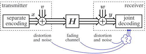
Fig. 1. System model for non-ideal MIMO communications with transmit and receive distortion. The receiver might be misinformed or ignorant of some of the variables in the transmission chain leading to mismatched decoding.
when considering their joint coupled effects or trying to model residual distortion after compensation. Thus, the binoisy signal model should be regarded as a compromise between facilitating theoretical analysis and resorting to measurements or simulations under more accurate modeling. Yet the central limit theorem further justifies the model by averaging the combined effects of different impairments to additive Gaussian noise when the signal model (1) is understood to represent a single narrowband subcarrier within a wideband system.
Additive receiver hardware impairments can be incorporated into the conventional signal model by increasing the level of the thermal-noise termnby a constant noise figure, e.g., about 3–5dB, or by scaling it in proportion to the input signal level such that it matches withw. On the other hand, regarding the joint effect of transmitter hardware impairments as an additive transmit-side noise term v is analogous to the principles of practical radio conformance testing. In particular, the common transmitter quality indicator is error-vector magnitude (EVM) which reduces the distortion effects to an additive component and measures its level relatively to signal amplitude [14].
Typical target EVM values guarantee that the signal x is at least 20–30 dB above the transmit-side noise v. On the other hand, for basic discrete channel inputs such as quadrature phase-shift keying (QPSK),Hxis usually at most10–15dB above the receive-side noisew, after which the communication is not anymore limited by noise but the lack of entropy in the modulation alphabet. This implies that transmitter hardware impairments can be justifiably omitted in the analysis of simple low-rate wireless systems: Either Hv is well below the receive-side noisew(say5–20dB) or the signal-to-noise ratio (SNR) is set to an uninterestingly high level. However, there has been a trend to improve data rates by using, e.g., quadrature amplitude modulation (QAM) up to 64-QAM at relatively high SNR, in which case the transmit-side noise begins to play a notable role in the link-level performance.
The considered system setup corresponding to (1) is shown in Fig. 1. As for MIMO processing, we focus on regular spatial multiplexing where a conventional transmitter separately en-codes and sends an independent stream at each of its antennas without having channel state information or being aware of the transmit-side noise it produces; the receiver jointly decodes the output signals of the MIMO channel knowing its instantaneous realizationHand some noise statistics. However, conventional receivers are designed and implemented based on the conven-tional signal model (wherev=0) due to which they are prone
to lapse into suboptimalmismatched decodingby inaccurately postulating the statistics of the actual noise term Hv+w. Even if off-the-shelf receivers can adapt to colored receiver noise, they may not be able to track the variable statistics of the componentHvpropagated from the transmitter since it is correlated with the fading channel. Only an advanced receiver would be able to performmatched decodingknowing perfectly the noise statistics as if it was designed and implemented explicitly based on the generalized binoisy signal model (1).
A. Related Works
The key reference results for the present study are re-ported in [2]–[11]. These seminal works originally formulated the research niche around (1) and established the baseline understanding of MIMO communication in the presence of transmit-side noise with numerical simulations and theoretical analysis. The majority of the related works, e.g., [2], [3], [6], [8], concern regular spatial multiplexing using separate encoding like the present paper but also different variations of joint encoding have been creditably investigated, e.g., in [4], [7]. On the other hand, all the studies that we are aware of assume (implicitly) advanced receivers that know the presence of transmit noise, no matter what form of decoding is used.
Especially, the reference results are polarized such that the scope of analytical studies [6], [8] typically differs from that of studies reporting simulations [6], [7], [9] or measurements [4]– [6]. Except for [2], practical discrete modulation schemes, e.g., QAM, have not been previously analytically evaluated in the presence of transmit noise, and simulation-based studies usually concern bit/symbol/packet error rates, not transmission rates which could be more interesting when studying modern adaptive encoding. In contrast, all the analytical capacity stud-ies assume Gaussian signaling and the throughput simulations of [3] with adaptive modulation and coding are their closest counterpart when it comes to experimental work.
If the receiver does not properly account for the additional transmit-side noise in the received signal, conventional mutual information (MI) is not anymore the correct upper bound for coded transmissions. Rather, due to mismatched decod-ing, one has to employ other metrics, such as generalized mutual information(GMI) [15], [16] adopted herein. Another common use for GMI is the analysis of bit-interleaved coded modulation [17], while also transceiver hardware impairments [18] and effects of imperfect channel state information at multi-antenna receiver [19], [20] are analyzed in terms of GMI. In particular, MI and GMI are evaluated herein using the replica method [21], [22], originating from the field of
statistical physics and introduced to the analysis of wireless systems by [23], [24]. Since then, the replica method has been applied to various problems in communication theory, e.g., MIMO systems [25]–[27]. For some special cases like Gaus-sian signaling, the replica trick renders exact asymptotic results when the number of antennas grows without bound, while they can be otherwise considered accurate approximations as shown by comparisons to Monte Carlo simulations.
B. Summary of Contributions
In this paper, we investigate two aspects of binoisy MIMO channels that are unexplored in related works despite their fundamental role in understanding the effects of hardware impairments in wireless systems. Firstly, analytical capacity results are limited to Gaussian signaling while practical digital modulation is evaluated only based on simple simulations or measurements. Secondly, the earlier literature focuses on the optimistic case of matched decoding by employing receivers that are actually not available off the shelf but implicitly updated to take account of transmit-side noise.
In particular, this paper contributes to the capacity theory of MIMO communication links by examining the effects of transmit-side noise as follows.
• Analytical GMI expressions are calculated for studying the rate loss of mismatched decoding when using a conventional receiver which is unaware of the transmit-side noise. Especially, it is shown that the performance remains the same irrespective of how well the noise covariance matrix is known if it is a constant.
• The above analysis is further translated into correspond-ing asymptotic high-SNR limits for Gaussian signalcorrespond-ing as a complement for the results of [10], which covers matched decoding and conventional MI.
• The analytical expressions provided for both conventional MI and GMI cover many practical discrete modulation schemes such as variations of PSK and QAM. This resolves the serious problem that evaluating (G)MI with direct Monte Carlo simulations for the present system is computationally infeasible except for cases with small number of antennas and low order modulation sets. Extending beyond the scope of the paper, the replica analysis of GMI is also a new aspect at large.
C. Outline of the Paper and Its Nomenclature
in Appendix A for the convenience of the reader. Appen-dices B contains general description of the replica method and Appendix C sketches the derivation of the main results in Section III.
Notation: Complex Gaussian random variables (RVs) are always assumed to be proper and the density of suchx∈CN with mean µand covariance R is denotedg(x|µ;R). For the zero-mean proper Gaussians, we say they are circularly symmetric complex Gaussian (CSCG). For convenience, both discrete and continuous RVs are said to have a probability density function (PDF) that is denoted by p, and we do not separate RVs and their realizations. For postulated PDFs we write q and add tilde on top of the related RVs (most of the time). Given a RVxthat has a PDFp(x), we writex∼p(x) (andx˜∼q(˜x)for the postulated case). Statistical expectation is denoted E{ · }and, unless stated otherwise, calculated over all randomness in the argument using true or postulated PDFs, depending on which type of RVs are present. Integrals w.r.t. real-valued variables are always over R (for vectors over the appropriate product space) and we tend to omit the integration limits for notational simplicity. For a complex variable z =
x+ jy, we denote R( )dz = R( )dxdy, and similarly for complex vectors. Logarithms are natural logs and denoted ln unless stated otherwise.
II. SYSTEM MODEL
Consider the system model depicted in Fig. 1 and the signal model of y ∈ CN written in (1) where H ∈CN×M is the channel matrix andx∈CM the signal of interest. The receive-side distortion plus noise component is divided into two parts, namely w = n+ω ∈ CN where n is caused by thermal noise andωrepresents hardware impairments arising from the non-ideal behavior of the radio-frequency (RF) transceivers. Similarly, v = m+ν ∈ CM where m and ν are related to thermal noise and hardware impairments or distortions, respectively, at the transmit-side. In practice, the effect of m is often negligible compared toν. In conventional MIMO literature it is common to consider only the thermal noise at the receiver, which translates to assuming ω =ν =m =0
in our more generic system model.
Let us denote the PDF of the transmit vectorxbyp(x)and assume it factorizes as
p(x) = M Y
m=1
p(xm), (2)
so that independent streams are transmitted at each transmit antenna. Furthermore, let p(xm) be a zero-mean distribution with varianceγ¯m. For later convenience, we letΓbe a diago-nal matrix whose non-zero elements are given by¯γ1, . . . ,γ¯M, that is, Γ = E{xxH}. The channel H is assumed to have
independent identically distributed (IID) CSCG elements with variance11/M. The thermal noise samples at the transceivers
1Typically the total power emitted from the transmit antennas in MIMO
systems is constant; that is,tr(Γ) = ¯γ, whereγ¯is some fixed power budget that does not depend onM. Hence the elements ofΓneed to be functions ofM in order to satisfy the transmit power normalization. For the following analysis, however, it is more convenient to treat the elements of Γ to be independent ofM and let the transmit power normalization be a part of the channel. Clearly, both approaches are mathematically fully equivalent.
are modeled as CSCG random vectors m and n that have independent elements. For simplicity, we assume that any given noise or hardware impairment component is independent of any other RVs in the system. The transmit- and receive-side impairments ν and ω are taken to be CSCG random vectors with covariance matrices Rν and Rω, respectively. The distortion plus noise vectors v and w are thus CSCG random vectors whose covariance matrices we denote Rv and Rw, respectively. Notice that these matrices can be functions of the statistics of some other RVs albeit we suppress the explicit statement of such dependence at this point for notational convenience. The SNR without transmit-side noise is defined astr(Γ)/tr(Rw).
The PDF of the received signal, conditioned on x, v and H, is given by
p(y|x,v,H) =g(y|H(x+v);Rw), (3)
and the receiver is assumed to know H and the true dis-tribution p(x) of the channel input. However, the additional transmit-side termv is in general unknown at the receive-side and, thus, the PDF (3) cannot be directly used for detection and decoding. Herein, we consider two different scenarios for the joint decoding operation at the receiver:
1) The receiver knows H, the PDFs of the noise plus distortion terms v andw as well as the distribution of the data vectorx.Matched joint decodingis then based on the conditional PDF
p(y|x,H) =Ev{g(y|H(x+v);Rw)} (4) =g(y|Hx; Rw+HRvH
H
), (5)
where the second equality follows by first using (62) to calculate the expectation w.r.t.v and simplifying the end result using (63) and (64). Note that the effective noise covariance matrix in (5) depends now on the instantaneous channel realization H.
2) The receiver has perfect knowledge of H and the PDF of the data vectorx. Instead of (4), however, the device uses a postulated channel law
q(y|x,H) =g(y|Hx; ˜R), (6)
for mismatched joint decoding [15], [16]. In contrast to Rw in (5), that is a random matrix, the postulated covariance matrix R˜ in (6) is fixed.
If matched joint decoding is employed, the conventional metric for evaluating the (ergodic) achievable rate of the system for given input distribution p(x) is the MI between the channel inputs and outputs, namely,
I(y;x) =E{lnp(y|x,H)} −E{lnp(y|H)}, (7)
III. MISMATCHEDJOINTDECODING: GENERALIZEDMUTUALINFORMATION
A. Definition and the Special Case of Gaussian Signaling
Let us assume that the received signal is given by (1) but the receiver uses (6) for decoding. Givenp(x), the (ergodic) GMI between the channel inputs and outputs is defined as [15], [16]
IGMI(y; x) = sup
s>0
IGMI(s)(y;x), (8)
where, denoting q(s)(y | H) =
Ex{q(y | x,H)s}, the s -dependent part reads
IGMI(s)(y;x) =E{lnq(y|x,H)
s
} −E{lnq(s)(y|H)}. (9) Since we consider ergodic rates, the expectations in (9) are w.r.t. all RVs in the system model, including the channel matrix H. If I is the maximum ergodic rate that can be transmitted over the channel (1) using input distributionp(x) and decoding rule (6), then I ≥IGMI [15], [16]. Herein, the
decoding based on the true channel law (4) cannot be obtained as a special case of the mismatched case sinceR˜ is fixed (see footnote 6 and (87) in Appendix C) and, thus, the case of matched decoding is considered separately in Section IV.
We are first interested in evaluating thes-dependent part of the normalized GMI per transmit stream M−1I(s)
GMI(y;x) for
given s > 0. The optimization over the free parameter s is carried out after the suitable expressions are found. The first term in (9) can be written as
1
ME{lnq(y|x,H)
s }
=−
=c(s)
z }| {
s M
Nlnπ+ ln det ˜R
− s
ME
(Hv+w)H˜
R−1(Hv+w)
=−c(s)−Ms
tr( ˜R−1Rw) + 1
M tr( ˜R
−1) tr(R
v)
. (10)
The first equality follows from (6) by the fact that y − Hx = Hv +w when x is given. The second equality is a consequence of the assumption that the channels and noise vectors are all mutually independent andHhas zero-mean IID entries with variance 1/M. Notice that (10) is independent of
p(x) and hence valid for all channel inputs. Evaluating the second term in (9) is more complicated but for the special case of Gaussian inputs we have the result shown below.
Example 1. For the special case of Gaussian inputs; that is,
p(x) =g(x|0;Γ),
1
MI (s)
GMI(y;x) =
1
MEH
ln det ˜R+sHΓHH
+str Rw+H(Rv+Γ)HH R˜+sHΓHH−
1
−str( ˜R−1Rw)−
s M tr( ˜R
−1) tr(R
v)−ln det ˜R
. (11)
The result is obtained by first using (62) and then simplifying with (63) and (64). Inserting the RHS of (1) into the obtained expression and taking the expectations w.r.t. the noise terms
v andw completes the derivation. ♦
Example 1 shows that for Gaussian signals we only need to average over the channel to obtain thes-dependent part of GMI. This is doable with Monte Carlo simulation. However, finding the optimalsis time consuming even in this case and a simple analytical expression that does not explicitly depend on the form of the marginals in (2) would be highly desirable. With this in mind, we adopt the following restriction to our system model from the physical characteristics of typical real transmitters for simplifying the analysis.
Assumption 1. The covariance matrix for the transmit-side distortion plus noise termv is diagonal so that we may write Rv = Rm +Rν = diag(r
(1)
v , . . . , r(vM)). Hence, v has independent (but not necessarily identically distributed) entries drawn according top(vm) =g(vm|0;r(vm)). ♦ The physical meaning of this assumption is that hardware impairments at different transmitter branches arise in separate electrical components and there are no mechanisms which generate significant correlation between the elements of the distortion noise vector. Furthermore, it is actually not neces-sary for the replica analysis but it helps simplify the end result to a form whose numerical evaluation is computationally easy.
B. Analytical Results via the Replica Method
If the goal is to calculate the expectations related to the latter term in (9) analytically and for general input distributions, we need to employ somewhat more advanced analytical tools than the basic probability calculus used in Example 1. As we shall see shortly, employing the replica method provides a formula that is applicable to a variety of input constellations, such as Gaussian or QAM. To begin, let us first denote
−1
MElnq
(s)(y|H) =c(s)+f(s), (12)
wherec(s)is defined in (10) and the latter term, equivalent of
the so-called free energyin statistical mechanics, reads
f(s) (13)
=−M1 EnlnEx˜
e−[H(x+v−x˜)+w]HsR˜−1[H(x+v−x˜)+w] o .
Now the inner expectation over the postulated channel input ˜
xis w.r.t. a generic PDF (2) and cannot be solved using (62) as before. The outer expectation is w.r.t. the rest of the RVs in the system, namely{x,v,w,H}. Due to (9) and (10) the expression to be optimized in the GMI formula thus becomes
1
MI (s)
GMI(y;x)
=f(s)−Ms
tr( ˜R−1Rw) + 1
M tr( ˜R
−1) tr(R
v)
. (14)
Remark 1. By (13) and (14), it is clear that if the receiver assumes that the additive noise in the system is spatially white
˜
R = ˜rIN with some finite sample variance ˜r, the GMI remains the same for all r >˜ 0 since the optimization over
The main obstacle in evaluating (14) is clearly f(s). This term happens to be, however, of a form that can be tackled by the replica method (see Appendix B). The following result is derived in Appendix C under the assumption of the so-called
replica symmetric (RS) ansatz when the system approaches the large system limit (LSL), that is, M, N → ∞ with finite and fixed ratio α = M/N > 0. The limit notation is omitted below and the results should therefore be interpreted as approximations for systems that have finite dimensions.
Proposition 1. Let m= 1, . . . , M and denote
χm=xm+vm, (15)
˜
χm= ˜xm, (16)
where xm,x˜m ∼ p(xm) and vm ∼ g(vm | 0;r(vm)) are
independent for allm by assumption. Let
p(zm|χm) =g(zm|χm;η−1), (17)
q(zm|χ˜m) =g(zm|χ˜m;ξ−1), (18)
be the PDF of an output zm of an additive white Gaussian
noise (AWGN) channel whose input is either (15) or (16), respectively, and corrupted by additive noise with variance η−1 orξ−1, respectively. The parameters η, ξ satisfy
η = 1
α
h
1
N tr ˜Ω−
1i2 1
N tr ˜Ω−1ΩΩ˜−1
, (19)
ξ= 1
αN tr ˜Ω
−1, (20)
for the given matrices
Ω=Rw+εIN, (21)
˜
Ω=s−1R˜ + ˜εIN, (22)
and variables
ε= 1
M
M X
m=1
E|vm+xm− hx˜miq|2 , (23)
˜
ε= 1
M
M X
m=1
E|x˜m− hx˜miq|2 . (24)
The notation hx˜miq above refers to a decoupled posterior mean estimator
hx˜miq = E˜xm{x˜mq(zm|x˜m)}
q(zm)
, (25)
where q(zm) =Eχ˜m{q(zm|χ˜m)}. If we also write p(zm) =
Eχm{p(zm | χm)}, the free energy f(s) defined in (14) is
given under the assumption of the RS ansatz by
fRS(s) =
1
αN
ln det ˜Ω+ tr ˜Ω−1Ω−ln det(s−1R)˜
−
lnπ
ξ + ξ η +
1
M
M X
m=1
Z
p(zm) lnq(zm)dzm
−ξε+ξ(ξ−η)
η ε.˜ (26)
If multiple solutions to the coupled fixed point equations(19)–
(24) are found, the one minimizing(26)should be chosen.
Proof: An outline of the derivation is given in Ap-pendix C.
The above result extends some previous works such as [23], [24] in the direction of correlated noise at the receiver and additive transmit-side impairments. It is thus clear that the original GMI term (9) of the MIMO system that suffers from transceiver hardware impairments has an interpretation in terms of an equivalent decoupled2 scalar system. This de-coupled channel has only additive distortions but unlike in the conventional case of replica analysis [23], [24], the transmit-side has its own noise term. It should be remarked, however, that the implicit assumption here is that fRS(s) =f(s); that
is, the system is not replica symmetry breaking (RSB). We leave the RSB case as a possible future work and check the validity of the solution with selected numerical simulations.
For simplicity of presentation, we consider next a few prac-tical special cases of Proposition 1 where the transmit power is the same for all antennas and the noise and distortions at the transmit-side are spatially uncorrelated, namely,Γ= ¯γIM andRv=rvIM. The receiver postulates spatially white noise
˜
R= ˜rIN with some variancer >˜ 0. This allows us to write 1
MIGMI(y; x) = sup˜s>0
n
f(˜s)−α−1˜s[N−1tr(Rw) +rv] o
,(27)
wheref(˜s)is given by (13) withsR˜−1replaced bys˜I
N. Fur-thermore, in this case all variables are identically distributed for allm= 1,2, . . . , M so we may omit the subscripts related tomin the following. We still need to fix the input distribution (2) to obtain the parameters (23) and (24). For this, we give two concrete examples: 1) Gaussian signaling; and 2) discrete channel inputs, such as, QAM.
Example 2. Let the channel inputs (2) be IID Gaussian, namely, p(x) = g(x | 0; ¯γIM) so that p( ˜χm) = p(xm) = g(x|0; ¯γ)andp(χm) =g(χm|0; ¯γ+rv)in Proposition 1. The parameterξ can then be obtained explicitly as
ξ=γ¯˜s(1−α)−α+ p
4αγ¯˜s+ [¯γs˜(1−α)−α]2
2α¯γ , (28)
whileη andεare obtained by solving the coupled fixed point equations
η= 1
α[N−1tr(R
w) +ε]
, (29)
ε= ηrv+ ¯γ(η+ξ
2γ¯) η(1 +ξ¯γ)2 =
¯
γ+rv (1 +ξγ¯)2 +
1
η(1 + 1/ξ¯γ)2. (30)
Additional algebra shows that for IID Gaussian inputs, the free energy (26) reduces to
fRS(˜s) =
1
α
ξ
η + ln ˜s+ ln
1
αξ
−ξε+ ln(1 +ξγ¯)+ ξrv 1 +ξ¯γ.
(31)
Note that the expression for parameter ε˜ in (24) is not explicitly given here but it is implicitly a part of (28) due
to relations (20) and (22). ♦
2This decoupling property is ubiquitous in replica analysis (see for example
TABLE I
HOW TOOBTAINGMIFORGAUSSIANSIGNALING FROMEXAMPLE2 1) Choose the parameters that define the MIMO system of interest, namely, antenna ratio α = M/N, transmit- and receive-side distortion plus noise covariance matricesRv =rvIM andRw, respectively, and the average transmit power per antenna¯γ. Let also the optimization parameter˜s >0be given.
2) Plug the values of{α,γ,¯ ˜s}to (28) and obtainξ.
3) Insert ξ along with the rest of the necessary parameters in (29) and (30), and solve η numerically, e.g., using an iterative substitution method.
4) Use the solutions ofξandηin (31) to obtain the free energy. 5) Optimize (27) overs >˜ 0.
The computational formula for obtaining the GMI with the above example is detailed in Table I. Notice that there are two non-trivial steps in the algorithm: 1) the optimization over s > 0; and 2) the problem of solving a system of two nonlinear equations with two unknowns. The first difficulty is not specific to the current study and is present in any work that considers GMI as means to analyze mismatched decoding. The computational complexity of the second problem is negligible compared to the original task of taking an expectation over the channel matrices in (11). Indeed, a typical solution for η
and εis obtained after some tens of iterations of an iterative substitution method.
For the high-SNR case where¯γ→ ∞for a fixed covariance matrix Rw, the result in Example 2 can be further simplified as shown in Example 3 below.
Example 3. Let us consider the case of Gaussian signaling as given in Example 2 in the limit γ¯ → ∞. We assume for simplicity (see, e.g., [10]) that Rw =rwIN and rv = ¯γκ2 where κ >0 and rw >0 are fixed and finite parameters. At high-SNR, there are two possibilities for the parameter s˜=
s/r˜in the GMI: 1) the optimal value ofs˜is a strictly positive constant; and 2) the value of˜sgoes to zero when¯γ→ ∞. For the first case,M−1I(s)
GMI(y;x)→ −∞so in order to obtain a
consistent solution for the fixed point equations, the parameter ˜
s has to be inversely proportional toγ¯, i.e.,s˜=sγ¯/γ¯ where sγ¯is a strictly positive finite constant. Thenξ→0as¯γ→ ∞,
and the normalized GMI reduces to 1
MI
∞
GMI(y; x) = sup
s¯γ>0
1
αln
s
¯
γ
αξγ¯
+ ln(1 +ξγ¯)
+ κ
2ξ ¯
γ 1 +ξ¯γ −
sγ¯κ2 α
, (32)
in the limit ¯γ→ ∞. The auxiliary parameterξ¯γ ,ξγ >¯ 0 is given by
ξγ¯=
s¯γ(1−α)−α+ p
4αsγ¯+ [s¯γ(1−α)−α]2
2α . (33)
Compared to the finite-SNR case in Example 2, the GMI is
now directly given by (32). ♦
The next example provides explicit formulas for the com-putation of GMI given finite discrete constellations, such as, PSK or QAM.
Example 4. Let A be a discrete modulation alphabet with fixed and finite cardinality|A|and consider the GMI (27). Let
the channel inputsxmbe drawn independently and uniformly from A. The parameters of the decoupled channel model in Proposition 1 can be obtained by first solvingξandε˜from
ξ= ˜s
α(1 + ˜sε˜), (34)
˜
ε= ¯γ− Z
q(z)|hx˜iq|2dz, (35)
using the following definitions for the decoupled estimator and the postulated channel probability
hx˜iq = 1
q(z)|A| X
˜
x∈A ˜
xg(z|x˜;ξ−1), (36)
q(z) = 1 |A|
X
x∈A
g(z|x;ξ−1), (37)
respectively. Note that this implies solving two parameters from two nonlinear equations and can be done, for example, by using an iterative substitution method. After obtaining the solutions for ξ (and ε˜), the rest of the parameters can be obtained by solving the two coupled equations
η= 1
α[N−1tr(R
w) +ε]
, (38)
ε=E|v+x− hx˜iq|2 , (39) for η and ε, where the expectation is w.r.t. the true joint probability of{x, v, z}. Finally, the free energy reads
fRS(˜s) =
1
α
ξ
η + ln ˜s+ ln
1
αξ
−ξε+ξ(ξ−η)
η ε˜
−
ξ η + ln
π ξ +
Z
p(z) lnq(z)dz
, (40)
where we denoted
p(z) = 1 |A|
X
x∈A
g(z|x;η−1+rv), (41)
for the decoupled PDF of the received signal. ♦
Notice that the form ofη in Example 4 is the same as in Example 2, but the parameterεhas now a different structure. Compared to the Gaussian case, the equivalent result for IID discrete channel inputs looks in general more cumbersome. First of all, we need to solve now two sets of equations instead of just one. They both contain terms that involve |A| summations and there are also two expectations left to evaluate, one in (35) and another in (39). However, both expectations involve only scalar variables. This is in stark contrast to the original problem that involved computing|A|M summations for every channel and noise / distortion realization and taking expectation over the channel and noise that are multidimensional integrals. This makes direct Monte Carlo computation of the GMI for discrete signaling in practice infeasible for large constellations and numbers of antennas.
IV. MATCHEDJOINTDECODING
A. Definition and the Special Case of Gaussian Signaling
I(y;x) =Mln|A| −N− 1 |A|
X
x∈AM
Ev,w,H (
ln X
˜
x∈AM
e−[H(x−x˜+v)+w]H(Rw+HRvH)−
1[H(x
−x˜+v)+w]
!)
(44)
receiver. The first entropy term in (7) reads
E{lnp(y|x,H)}=−EH{ln det(Rw+HRvHH)} −c, (42) wherec=Nln(eπ). It should be remarked that there is still an expectation left w.r.t. the channel realizationsH in (42). This could be evaluated, for example, using Monte Carlo methods or random matrix theory [28], [29]. For the special case of Gaussian inputs, the identities in Appendix A allow us to partially calculate also the latter entropy term in (7), providing the following result that is useful for Monte Carlo simulations.
Example 5. Letp(x) =g(x|0;Γ). Then,
1
MI(y;x) =
1
MEH{ln det(Rw+H(Γ+Rv)H
H
)}
−M1 EH{ln det(Rw+HRvHH)}, (43)
is the normalized ergodic MI for matched decoding. ♦
The above expression is relatively easy to compute also by brute-force Monte Carlo methods since there is only an expectation over the fading. Unfortunately, to the best of our knowledge, the latter entropy term in (7) is mathematically intractable for rigorous methods like random matrix theory when p(x) is an arbitrary distribution that satisfies (2). For example, given discrete inputs as in Example 4, calculating
E{lnp(y | H)} and combining it with (42) reduces the MI to (44) given at the top of this page. This form is computationally very complex and can be evaluated using Monte Carlo methods only for small number of antennas and simple constellations. To obtain a result for general input distributionp(x)that has lower computational complexity, we resort to the replica method (see Appendix B). As before, the results that follow have been written in a simplified form where the assumption of LSL is suppressed for notational simplicity.
B. Analytical Results via the Replica Method
Proposition 2. Let us write for notational convenience
χm=xm+vm, m= 1, . . . , M, (45)
where xm ∼ p(xm) and vm ∼ g(vm | 0;rv(m)) are
independent for allm. Let
p(zm|χm) =g(zm|χm;η−1), (46)
be a conditional PDF of an AWGN channel whose input is(45)
and noise variance isη−1. The conditional mean estimator of χmreceived over this channel reads
hχmi=Eχm{χmp(zm|χm)}
Eχm{p(zm|χm)}
, (47)
where the parameterηis given, along with another parameter ε, as the solution to the coupled fixed point equations
η= 1
αN tr
(Rw+εIN)−1
, (48)
ε= 1
M
M X
m=1
¯
γm+rv(m)−E|hχmi|
2.
(49)
If we also define a second set of parametersη′andε′ that are
solutions to the coupled fixed point equations
η′= 1
αNtr
(Rw+ε′IN)−1, (50)
ε′= 1
M
M X
m=1 r(vm)
1 +η′r(vm), (51)
the per-stream MI is finally given by
1
MI(y;x) =
ln det(Rw+εIN)−ln det(Rw+ε′IN)
αN
−(ηε−η′ε′) + 1
M
M X
m=1
I(zm;χm)−ln(1 +η′r(vm))
, (52)
where
I(zm;χm) =−1−ln
π η −
Z
p(zm) lnp(zm)dzm, (53)
is the MI of the Gaussian channel defined by(45) and (46).
Proof: The result can be obtained using Appendix B for two separate MIMO channels. For the first one, we replace everywhere xa → xa+va, a= 0,1, . . . , u and and an application of the RM provides the equations (45)–(49). The formulas (50)–(53), on the other hand, are obtained by substitutingxa→va, a= 0,1, . . . , uin Appendix B.
Just like Proposition 1 in Section III, Proposition 2 is valid for any input distribution that satisfies (2). The solutions to the coupled equations (48) and (49) as well as (50) and (51) can be obtained numerically, e.g., using an iterative substitution method.
For concreteness, we again give examples for Gaussian and discrete signaling when the noise plus distortion is spatially whiteRv=rvIM and transmit power is uniformly allocated
Γ = ¯γIM. This makes the channels m = 1,2, . . . , M
identically distributed so we omit the subscript m in the following.
Example 6. Let Rv = rvIM and consider the special case of Gaussian inputsp(x) =g(x|0; ¯γIM). Then
I(z;χ) = ln1 +η(¯γ+rv)
, (54)
ε= ¯γ+rv 1 +η(¯γ+rv)
, (55)
We next consider the high-SNR case γ¯ → ∞ as in Example 3 and compare it to the result obtained in [10] using completely different mathematical methods.
Example 7. For the caseRw=rwI,Rv=κ2γ¯I (see, e.g., [10]) we find that if α≤ 1 then ¯γ → ∞ yields η =η′ and
ε=ε′. The high SNR limit is therefore
1
MI
∞(y;x) = log
1 +κ2 κ2
, α≤1. (56)
For the case α >1, bothη andη′ tend to zero at high SNR whileεandε′grow without bound. This is not yet sufficient to solve (52). However, combining this with the relationsη′ε′=
ηε andε′=ε κ2
1+κ2, that hold in the limit¯γ→ ∞ for α >1, provides the second part of the high SNR result
1
MI
∞(y;x) = 1
αlog
1 +κ2
κ2
, α >1. (57)
The asymptotic mutual information expressions in (56) and (57) coincide exactly with the results obtained previously in
[10], as expected. ♦
Example 8. If the channel inputs are from a discrete alphabet Aas in Example 4, the parameterεin (49) is obtained using
hχi= 1
p(z) X
x∈A
1
|A|g(z|x;η −1+r
v)
x+ηrvz 1 +ηrv
, (58)
E|hχi|2= Z
p(z)E|hχi|2 dz, (59)
in Proposition 2. Herep(z) is given by (41) andhχidenotes the conditional mean estimator of (45) from the observations (46). The related MI term reads by definition
I(z;χ) = ln
η
eπ
−
Z
p(z) lnp(z)dz. (60)
Both (49) and (60) need, in general, to be solved numerically.♦
V. NUMERICALEXAMPLES
In the following, assume for simplicity that Γ = ¯γI,
Rw = I and Rv = κ2γ¯I, where κ = 10EVM/20 and
EVM denotes the EVM of the transmitter in decibels. The SNR without transmit-side noise is therefore simply γ¯, or in decibels, ¯γdB = 10 log10(¯γ). Furthermore, all cases assume a
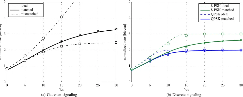
symmetric antenna setupα=M/N = 1for simplicity. The first numerical experiment plotted in Fig. 2 examines the accuracy of the asymptotic analytical results when applied to finite-sized systems. The EVM is fixed to a rather pes-simistic value EVM = −10 dB to highlight the differences between the ideal and imperfect hardware configurations. The normalized rate is shown using the asymptotic replica analysis (lines) and Monte Carlo simulations (markers) for a finite-size symmetric antenna setup with M = N = 4. In the case of Gaussian signaling, plotted in Fig. 2(a), the analytical approximations for the normalized rateM−1I(y;x)given by
Examples 2 and 6 are quite good when compared to the finite size simulations based on Examples 1 and 5. For discrete signaling depicted in Fig. 2(b) we have plotted only the case of matched decoding due to the computational complexity
of Monte Carlo simulations in the mismatched case. The gap between asymptotic result presented in Example 8 and Monte Carlo averaging of (44) is similar to the Gaussian case for both constellations. Figure 2 shows that the analytical approximation given by the replica method is reasonably good already at M = N = 4, even though formally the limit
M, N → ∞is required by the analysis. Note that Monte Carlo simulation of (44) has exponential computational complexity and the system size cannot be increased much higher than
M = 4. Therefore, the rest of the examples are generated using only the analytical results given in the previous sections. Figure 3 illustrates the performance of anM =N MIMO system for a more realistic EVM value EVM=−20 dB. For the case of matched decoding we used Examples 6 and 8, while Examples 2 and 4 were used to obtain the curves representing mismatched decoding. In Fig. 3(a), the normal-ized rate M−1I(y;x) is depicted as a function of SNR
¯
γ in decibels. For clarity of presentation, we have plotted only the ideal case and the case of non-ideal hardware with matched decoding. The Gaussian curves (black lines) here are the same as the simulation curves in [10, Fig. 2] given the parameter value κ = 0.1. Apart from 64-QAM and Gaussian signaling, the figure seems to imply that lower order constellations exhaust the source entropy before the transmit-side noise has any significant effect for this choice of EVM. To see more clearly the effect of transmit noise, Fig. 3(b) shows the rate loss (in percentage) for the case with transmit noise EVM = −20 dB when compared to the ideal case
EVM = −∞ dB. The solid lines represent again matched decoding while dash-dotted lines are for mismatched decoding. As expected, mismatched decoding reduces the achievable rate when compared to matched decoding, but the effect is relatively minor when compared to the total rate loss caused by the presence of transmit noise itself. The markers depict the points where maximum relative rate loss is experienced for matched decoding. The same markers are also plotted in Fig. 3(a) for comparison.
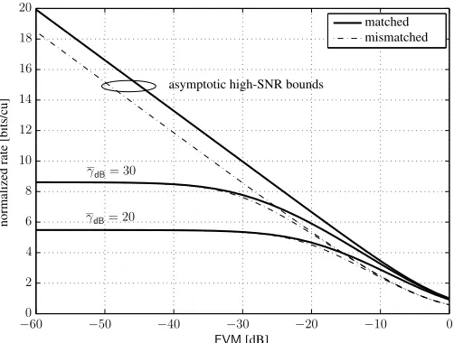
In Fig. 4 we have plotted the asymptotic high-SNR results given in Examples 3 and 7. Note that given a finite value of EVM, the normalized rates for matched and mismatched decoding have a gap in this case. For more realistic, but still quite high SNR values of20dB and30dB, the two decoding strategies converge to the same value roughly when γ¯dB <
−EVM. The apparent discrepancy is explained by recalling that the asymptotic cases assume γ¯ → ∞ for a fixed and nonzero EVM and, thus, as a finite SNR approximation implies ¯
γ ≫1/κ2. As may be observed from the lower right corner
of the figure, the SNR values 20 dB and 30 dB have also a similar behavior near γ¯ ≫1/κ2. Thus, the high-SNR result
is consistent with the finite-SNR cases.
mismatched matched ideal
n
o
rm
al
iz
ed
ra
te
[b
it
s/
cu
]
γdB
0 5 10 15 20 25 30
0 1 2 3 4 5
(a) Gaussian signaling
QPSK matched QPSK ideal 8-PSK matched 8-PSK ideal
n
o
rm
al
iz
ed
ra
te
[b
it
s/
cu
]
γdB
0 5 10 15 20 25 30
0 1 2 3 4 5
[image:10.612.59.553.63.261.2](b) Discrete signaling Fig. 2. Normalized rateM−1
I(y;x)in bits per channel use (cu) vs. SNR for MIMO transmission. Lines for replica results and markers for Monte Carlo simulations forM =N= 4antenna configuration. Selected cases of ideal hardwareEVM=−∞dB and hardware impairments (EVM=−10dB) with matched and mismatched decoding are plotted.
QPSK 16-QAM 64-QAM Gaussian
n
o
rm
al
iz
ed
ra
te
[b
it
s/
cu
]
γdB
0 5 10 15 20 25 30
0 1 2 3 4 5 6 7 8 9
(a) Normalized rate M−1
I(y;x) given ideal hardware (dashed lines) or non-ideal hardware and matched decoding (solid lines).
QPSK 16-QAM 64-QAM Gaussian
ra
te
lo
ss
%
γdB
0 5 10 15 20 25 30
0 5 10 15 20 25 30
(b) Rate loss percentage compared to ideal hardware for matched (solid lines) and mismatched (dash-dotted lines) decoding.
Fig. 3. Performance of a MIMO system withM=Nantennas and given ideal (EVM=−∞dB) or non-ideal hardware (EVM=−20dB) for different signaling methods. Markers depict the points where discrete constellations and matched decoding with hardware impairments experience the maximum rate losses compared to the ideal cases.
linear, function of SNR. A simple linear approximation that provides a lower bound for the case of Gaussian signaling with matched decoding is given by
EVM=−0.7·¯γdB−13, (61)
in decibels for the depicted region. This can be used as a simple rule-of-thumb for worst-case maximum allowed EVM in the system, although we recommend that EVM target values obtained in this way are always rounded down to1–5dB preci-sion to include extra safety margin. For discrete constellations, the EVM requirement first follows the Gaussian case but then starts to get looser at higher SNRs. This is expected, as can be observed from Fig. 3(a), since the maximum achievable rate for a discrete constellation saturates at a certain SNR when
the input distribution runs out of entropy. After this point, the rate loss can be held fixed for increasing SNR by increasing the transmit-side noise variance, or EVM, accordingly.
VI. CONCLUSIONS ANDFUTUREWORK
[image:10.612.57.555.315.504.2]mismatched matched
n
o
rm
al
iz
ed
ra
te
[b
it
s/
cu
]
EVM[dB]
γdB= 20 γdB= 30
asymptotic high-SNR bounds
−60 −50 −40 −30 −20 −10 0 0
[image:11.612.50.301.52.242.2]2 4 6 8 10 12 14 16 18 20
Fig. 4. Normalized rate M−1
I(y;x)in bits per channel use vs. EVM in decibels for MIMO transmission with Gaussian signaling. Solid lines for matched decoding and dash-dotted lines for mismatched decoding.
Gaussian mismatched Gaussian matched 64-QAM,(22.5,−28.2)
16-QAM,(15.3,−22.9)
8-PSK,(12.0,−19.7)
QPSK,(6.5,−16.4)
m
ax
im
u
m
E
V
M
fo
r
5
%
ra
te
lo
ss
γdB
0 5 10 15 20 25 30
−35
−30
−25
−20
−15
−10
[image:11.612.50.299.292.486.2]−5
Fig. 5. Maximum allowed EVM in decibels for matched decoding so that the system experiences at most 5% loss in rate compared to the case with ideal hardware (EVM = −∞ dB). Markers depict the worst case EVM requirement for the discrete constellations and parenthesis in the legend provide the respective values as(¯γdB,EVM). All discrete cases correspond
to matched joint decoding at the receiver.
studied via generalized mutual information. The mathematical expressions provided in the paper cover practical discrete mod-ulation schemes, such as, quadrature amplitude modmod-ulation, as well as Gaussian signaling. The numerical results showed that for realistic system parameters, the effects of transmit-side noise and mismatched decoding become significant only at high modulation orders. Furthermore, the effect of mismatched decoding was found to be relatively minor compared to the total rate loss caused by the presence of transmit noise itself. The results were also used to identify the maximum EVM values that allows for certain system operation.
A. Future Work
For the ease of exposition, the present paper considered the analysis of a relatively simple SU-MIMO system where
the channel had IID Gaussian elements. An extension of the replica analysis to Rayleigh fading channels with Kronecker correlation can be done by following, e.g., the derivations in [26]. Establishing the effects of transmit-side noise for the case of correlated channel is an important avenue for future work. As a further extension, it is important to investigate whether similar phenomena as observed in the present paper are present also for more complicated signal models with discrete channel inputs. Such systems already analyzed in the ideal setting with the replica method include, for example, multiuser MIMO and base station collaboration [30], channels with interference and precoding [31] andK-hop relay channels [32]. Combining the ideas from the present paper and [30]–[32] would provide a possible approach to solving such cases.
APPENDIXA USEFULRESULTS
Here we collect useful results that are used often in the paper. All matrix operations below are implicitly assumed to be well-defined. The Gaussian integrationformula for vector x∈CN is given by (see, e.g., [33, Appendix I])
1
πN Z
e−xHM x+2ℜ{bHx}dx= 1 det(M)e
bHM−1b
, (62)
and used in Sections II – IV and Appendix C. Similarly, the
matrix inversion lemma[34]
(W−1+U T−1VH)−1
=W −W U(T+VHW U)−1VHW, (63) and the relateddeterminant identity
det(W−1+U T−1VH)
= det(T+VHW U) det(W−1) det(T−1), (64) are employed several times in the paper.
APPENDIXB REPLICAMETHOD
Consider a function Z that maps RVs to real numbers3 and define two sets of RVs, V ∈ V and X ∈ X, with joint probabilityPV,X. Assume for convenience thatPV,X can be described in terms of a joint PDF p(V, X) and denote the marginal PDFs ofX andV pX(X)andpV(V), respectively. Then, both in statistical mechanics and communication theory, we often encounter a formula
f =− 1
MEV
lnEX{Z(V, X)}
=− 1
M
Z
V
pV(V) lnZ(V) dV, (65)
whereZ(V) =RXpX(X)Z(V, X)dX. In physics jargon, the variablesV are said to bequenched and the quantity (65) is the average free energy densityof a system whose partition functionisZ(V). Two concrete examples of (65) are:
3In the following we refrain differentiating random variables and their
1) Let Z(V, X) = g(y | Hx;Rw) be the conditional PDF of the observation in an ideal MIMO channel with
V ={y,H} andX ={x}, wherex has IID elements from a discrete modulation setA, such as PSK or QAM. Then (65) represents a normalized version of the second term in (7), namely, the (normalized) totalentropyof the received signalygiven a realization ofH and averaged over all possible realizations ofH.
2) Let Z(V, X) = eβσH
J σ, where β > 0 denotes the inverse temperature,V =J ∈RM×M a coupling matrix andX =σ ∈ {±1}M a spin configuration. If p
V(V) is a uniform probability over σ and J has, e.g., IID Gaussian elements, then (65) is the averagefree energy density of a mean-field Ising spin glass in the absence of external field (up to trivial constants).
In both cases, f captures important properties of the system at hand and obtaining a computable formula for (65) would be of great interest. This seems infeasible though since the number of terms in the expectation is exponential inM.
A. Outline of the Replica Method
One method for solving (65) is the replica method (RM) from equilibrium statistical mechanics. While the RM is extremely versatile, it unfortunately lacks mathematical rigor in some parts (see, e.g., [21]–[23]). However, due to its success both in physics and engineering, it is generally agreed to be at least a valuable starting point for analysis of problems that seem otherwise too difficult to handle. A cursory overview of literature about the RM inside a specific field or topic may paint the picture that the RM is a fixed set of mathematical methods which can be applied to any suitable problem at hand. This is not entirely accurate and conceptually the RM can be seen more like a systematic way of turning a very difficult problem into a more manageable one than a set of specific tools that actually solve the problem. Indeed, the mathematical methods that are used at different stages of the RM can often be chosen from a variety of choices, although it is very common to have some form oflarge deviations theory
as part of the analysis (see Step 2 below). Thus, instead of trying to be entirely general, we describe next (one form of) the steps taken in the RM in the context of the first example above.
Step 1 (Replica trick). Consider (65) and write it as
f =−1
M ulim→0+
∂
∂ulnEV{[Z(V)]
u }
=−M1 lim u→0+
∂ ∂ulnEV
X
x∈AM
pX(x)Z(V,x)
u
=−M1 lim u→0+
∂
∂uln Ξ(u), (66)
where u∈ R and we denoted Ξ(u) =EV{[Z(V)]u}. Then,
assume that we can treat u as an integer when we take the
expectation, namely,
Ξ(u) =EV
u
Y
a=1
X
xa∈AN
pX(xa)Z(V,xa)
(67)
= 1
πuN(detR w)u
×EV
X
{xa}
u Y
a=1
e−(y−Hxa)
H R−1
w (y−Hxa)p
X(xa)
,
where the summation in the last expression is over the set {xa}ua=1. After taking the expectations, if we manage to write
(67) in a form that does not explicitly forceuto be an integer,
invoke analytical continuityto extend uto real numbers. ♦
The step above is at the very heart of the RM. It is important to realize that the equalities in (66) are provably true if differentiation under the integral sign is permitted andu∈R. The part lacking rigorous mathematical justification is (67), especially when combined with the next two steps. Somewhat surprisingly, however, the end results of RM can sometimes be proved to be exact. Examples of such cases are: MIMO channel with Gaussian inputs, random energy model (REM) and Sherrington-Kirkpatrick model of spin glasses (see, e.g., [21]–[24] and references therein).
Step 2 (Large system limit). Let the system approach the LSL, that is, the dimensions of the channel matrix H grow without bound at a finite and fixed ratio α = M/N > 0. Furthermore, assume that the limits w.r.t.uandM commute, so that we can first calculate the expectations in (67) in the
LSL and then letu→0, as in (66). ♦
The LSL assumption is natural in equilibrium statistical mechanics (e.g. the second example above), where the systems contain usually very large numbers of interacting particles
M. In communication theory, the equivalent would be, e.g., a MIMO systems with large antenna arrays or a CDMA with large number of simultaneous users. It is in fact quite common to write the LSL assumption directly as a part of the replica trick in (66). The steps are separated here since the replica trick could also be used for finite sized systems. Due to mathematical difficulty of such cases, however, both steps are usually found together. The assumption of commuting limits is typically postulated a priori and rigorous justification of this step is beyond the scope of this paper.
Let us denote the true transmitted vector x0, so that
y =Hx0+w is the generating model for the observation
yand we can equivalently write V ={w,x0,H}. Returning
then to Step 1, we note that although the replicated vectors {xa}ua=1 act as IID RVs drawn according topX in (67) when conditioned on V, they can be correlated if not conditioned on V. We examine this through the empirical correlations between the vectors in the setXu+1={xa}ua=0usingoverlap matrix Q ∈ C(u+1)×(u+1), whose (a, b)th element4 is given
byQa,b=M−1xHbxa. Then, the structure that is imposed on
4The row/column indexes ofQare0,1, . . . , uso that the correlations are
measured also w.r.t. the true transmitted vectorx0. Furthermore, due to (2),
Q divides the replica analysis into two rough categories as described below.
Step 3 (Replica symmetry). The RS ansatz or RS assump-tion means that the indexes a = 1, . . . , u are permutation symmetric andQcan be written in terms of four parameters, for example, Q0,0=p,Q0,a =m, a≥1, Qa,a=Q, a ≥1, andQa,b=q, a6=b≥1. Note thatQ=QH by construction. If Q is not of the RS form, it is said to have replica symmetry breaking (RSB) structure whose analysis is much more involved [21], [22].
The importance of the RS assumption will become clear when we present a rough sketch of the analysis of an ideal MIMO channel. We also note that the overlap matrix given in
Step 3 allows the “zeroth” index to be treated separately to take into account the possibility that eitherx0has different
dis-tribution thanxawhena≥1, or the decoder uses mismatched statistics, i.e.,Z(V,xa)does not match the probability law of the observation y = Hx0+w as in Appendix C. For the
simplified case considered below, however, we have p = Q
and m =q since the indexes a = 0,1, . . . , ucan be treated on equal footing and two parameters is sufficient to define the RS form of Q.
Next we give a brief and informal example of replica analysis for ideal MIMO channel. The reader may be surprised to find out that most of the discussion below deals with details about how to obtain the necessary formulas when we follow the three stages above and not about those stages per se.
B. Average Over the Channel and Noise
The starting point of our replica calculations is (67), where we use the generating model of y to write in the exponential y−Hxa=w−H(x0−xa). The first task is then to compute the expectation w.r.t.w andH for a fixedXu+1={xa}ua=0
that satisfies the correlations of the RS overlap matrixQ. Note that we cannot assume anymore that the vectors inXu+1 are
independent since we changed the order of expectations in (67) and the average over Xu+1 is carried out (later) without
conditioning on w and H. With this in mind, it follows that given Xu+1, the set {Hxa} consists of CSCG RVs
with correlations EH{(Hxa)(Hxb)H} = M−1xHbxaIN =
Qa,bIN that are deterministic in the LSL. Thus, we can replace {H(x0 −xa)}ua=1 by a set of CSCG RVs {∆a}ua=1 and
use Gaussian integration (62) to average over both w and {∆a}ua=1 to obtain (for details, see Appendix C-B.)
Ξ(u) = Z
eN G(u)
(Q)µ(Q)dQ, (68)
G(u)(Q) =−uln det[Rw+ (Q−q)IN]
−ulnπ−ln(u+ 1) (69)
where Q should be understood to be in its RS parametrized form and µ(Q)is the PDF of the overlap matrix Q.
Remark 2. Firstly, note that due to the RS assumption (Step 3), the function (69) is of a form that does not restrict
uto be an integer, as desired. This is one of the reasons why we need to express matrix Q in a parametrized way instead
of using it “as-is”. Secondly, there is some universality in this derivation and the form (68) is a typical result of replica analysis. In some cases, however, different techniques are needed. One example is non-IID “mixing matrix” that requires
direct matrix integration [35], [36]. ♦
C. Distribution of the Overlap Matrix and Large Deviations
The second major step in the analysis is to find an explicit formula for µ(Q), i.e., for the probability weight of the set {xa}ua=0 that satisfies Qa,b =M−1xHbxa. The form of (68) suggest that we should try to representµ(Q)as an exponential whose argument is linear inN (orM) so that we can employ Laplace’s method or the method of steepest descent to evaluate the integral w.r.t. Q. If xa ∈ RM, due to (2), the elements of xa are IID for alla= 0,1, . . . , u andµfollows the large deviation principle [22], [37]. Informally this implies5µ(Q)≍
e−M c(u)(
Q), where therate function
c(u)(Q) = sup
˜
Q
tr(QQ)˜ − lim M→∞
1
M lnφ (u)( ˜Q)
, (70)
describes the exponential behavior of the probability,
φ(u)( ˜Q) =EXu+1
exp
u
X
a,b=0
˜
Qa,bxHbxa
, (71)
is the moment generating function (MGF) associated with
µ(Q)and the supremum is over all(u+ 1)×(u+ 1)matrices ˜
Q that have the same RS form as Q, that is, Q˜0,0 = ˜p,
˜
Q0,a= ˜m, a≥1,Q˜a,a= ˜Q, a≥1,andQ˜a,b = ˜q, a6=b≥1. Thus, we can assess (68) in the LSL up to the leading order by using the exponential form of µ and Laplace’s method, namely,
Ξ(u)≍ Z
eM α−1G(u)(Q)
e−M c(u)(Q)dQ
= Z
exp N[α−1G(u)(Q)−c(u)(Q)]dQ (72)
≍exp
Msup Q,Q˜
T(u)(Q,Q)˜
, (73)
where we denoted for notational convenience
T(u)(Q,Q) =˜ 1 αG
(u)(Q)−tr(QQ) + lim˜
M→∞ 1
M lnφ (u)( ˜Q).
(74) For complex vectors {xa}, the end result is essentially the same and the solution to the supremum is found among the critical points of the argument (see e.g., [26], [27], [35]). The large deviations analysis also guarantees that Q˜ is in general a real symmetric matrix and if (Q∗,Q˜∗) is the solution of the optimization problem in (73) then T(u)(Q∗,Q˜∗)∈R, as expected sincef is in our case real.
However, in RM there is some ambiguity as to whether the correct point in the saddle-point approximation (73) minimizes or maximizes the exponential when we letu→0 [21], [22].
5We use notation a
M ≍ bM to denote “equality up to the leading
exponential order”, that islimM→∞M −1
Thus, in RM, we seek in practice the critical points and (66) is thus of the form
f =− lim u→0+
∂ ∂uextrQ,Q˜
T(u)(Q,Q)˜ , (75)
where extrX{h(X)} denotes finding the critical points of a functionh(X).
D. Decoupled MGF and Critical Points
The second part of replica analysis where the RS assumption plays an important role (for the first one, see Remark 2) is when we try to solve (71) and find the critical points of
T(u)(Q,Q). For the simplified setup in this section where˜
Q andQ˜ are represented with parameter {Q, q} and{Q,˜ q˜}, respectively, the MGF can be expressed as (see, e.g., [24] for details)
φ(u)( ˜Q) = M Y
m=1
" ˜
q π
−uZ
Exmg(zm|xm; ˜q
−1)u+1
dzm #
,
(76)
wherezmare just dummy variables. On the other hand, finding the critical points involves taking eight partial derivatives for the RS case in Step 3 (for the simplified case here, four is enough). Then, one should pick the solution that satisfies the conditions at the critical point while providing the global extremum of (66). In the case considered here, we can actually get rid of two parameters since p =M−1
Ekxk2 andp˜= 0
always at the critical point. Note that if we did not parametrize Q, the critical points would be described byu(u+1)equations and Ξ(u) would depend explicitly on the fact that u is an integer. This is one of the reasons why even the full-RSB solution (see [21], [22]) uses a round-about way of presenting Q instead of using it “as-is”.
Finally, we remark that it is quite common (see, e.g., [24]) to represent the end result in terms of new variables. For example, if we have equal transmit powers for each antennas¯γ= ¯γmin the simplified case considered here, then the parametersη= ˜q
andε=Q−q= ¯γ−qfully describe the RS matricesQand ˜
Q at the critical point. The former variable is inverse noise variance of a decoupled Gaussian channel
z=x+w, p(w) =g(w|0;η−1), (77)
and the latter variable ε is the MMSE of this channel when the inputs are drawn according to pX(x). The rest of RM is straightforward, albeit tedious algebra to arrive at (66).
APPENDIXC
REPLICAANALYSIS FORMISMATCHEDCASE
The analysis herein follows the main steps of RM as listed in Appendix B. Reader who is not familiar with the RM is encouraged to use discussion there as a guide to the derivations below.
A. Replica Trick
Let us consider the function f(s)(free-energy) defined in (13). We then postulate that it can be expressed in the LSL using the standard replica trick (cf. Appendix B)
f(s) =− lim M→∞
1
M ulim→0 ∂ ∂uln Ξ
(u,M)(s),
(78)
where we defined for later convenience
Ξ(u,M)(s) =E
u
Y
a=1
e−[w+H(χ0−χa)]
H
Σ−1[w+H(χ0−χ
a)]
,
(79) and denoted6 Σ = s−1R˜ along with χ
0 = x0 +v0 and
χa = xa, a = 1, . . . , u. Here x0 is the original
trans-mit vector in (1) and {xa}ua=1 are replicated data vectors,
which are IID drawn according top(x)when conditioned on {x0,v0,w,H}. On the other hand, v0 represents the noise
plus distortion component at the transmit-side that is CSCG with covariance matrixRv. Starting with (79), the goal is then to obtain a functional expression forΞ(u,M)(s)in the LSL that
does not enforceuto be an integer and then use (78) to obtain the desired quantity. In the following, explicit limit notations are often omitted for notational convenience.
B. Average Over the Channel and Noise
To proceed with the evaluation of (79), we first make the RS assumption
p=M−1kχ
0k2, (80)
m=M−1χH0χa, a= 1, . . . , u, (81)
Q=M−1kχak2, a= 1, . . . , u, (82)
q =M−1χHaχb, a6=b∈ {1, . . . , u}. (83)
and remind the reader that if we average first over H, the empirical correlations between {xa}u
a=0 are not zero in
general as discussed in Appendix B. Thus, noticing that
EH{[H(χ0−χa)][H(χ0−χb)]H}
= (
p−(m+m∗) +QI
N, a=b,
p−(m+m∗) +qIN, a6=b, (84)
we may replace {H(χ0−χa)}ua=1 in (79) in the LSL by
CSCG vectors{∆a}ua=1 that are constructed as
∆a =dapQ−q+tpp−(m+m∗) +q (85)
=da √
A+t√B, (86)
wheret,{da}u
a=1 are IID standard complex Gaussian RVs
independent ofw. Plugging (86) intoΞ(u,M)(s)and recalling
6 We remind the reader that for the case of mismatched decoding, the
postulated covariance matrixR˜ is fixed by definition so thatΣ= s−1˜
R