White Rose Research Online
eprints@whiterose.ac.uk
Universities of Leeds, Sheffield and York
http://eprints.whiterose.ac.uk/
This is an author produced version of a paper accepted for publication in
IEEE Transactions on Ultrasonics Ferroelectrics and Frequency Control.
White Rose Research Online URL for this paper:
http://eprints.whiterose.ac.uk/43139/
Paper:
Cowell, DMJ and Freear, S (2010)
Separation of Overlapping Linear Frequency
Modulated (LFM) Signals Using the Fractional Fourier Transform.
IEEE
Separation of Overlapping Linear Frequency
Modulated (LFM) Signals using the
Fractional Fourier Transform
D M J Cowell, and S Freear,
Member, IEEE
Abstract—Linear frequency modulated (LFM) excitation com-bined with pulse compression provides an increase in signal to noise ratio (SNR) at the receiver. LFM signals are of longer du-ration than pulsed signals of the same bandwidth. Consequently, in many practical situations, maintaining temporal separation between echoes is not possible. Where analysis is performed on individual LFM signals, a separation technique is required. Time windowing is unable to separate signals overlapping in time. Frequency domain filtering is unable to separate signals with overlapping spectra. This paper describes a method to separate time overlapping LFM signals through the application of the fractional Fourier transform (FrFT), a transform operating in both time and frequency domains. A short introduction to the FrFT, its operation and calculation are presented. The proposed signal separation method is illustrated by application to a simulated ultrasound signal, created by the summation of multiple time overlapping LFM signals and the component signals recovered with ±0.6% spectral error. The results of an experimental investigation are presented where the proposed separation method is applied to time overlapping LFM signals, created by the transmission of a LFM signal through a stainless steel plate and water-filled pipe.
I. INTRODUCTION
I
N many ultrasound measurement systems, time and fre-quency analysis methods operate on individual ultrasonic signals and are unable to support signals overlapping in time. Individual ultrasonic signals must be separable. When multiple signals have a temporal overlap, time domain windowing is unable to provide a method of signal separation. Frequency domain filtering is unable to provide signal separation due to the similarity between spectra of the ultrasound echo signals. Frequency domain analysis of time overlapping signals using the Fourier transformation does not produce the spectrum of the individual signals. The frequency-phase relationship of the individual signals is incoherent causing periodic constructive and destructive interference, resulting in a spectrum with irregular characteristics that is representative of the combined signal rather than the individual ultrasound signals.Time overlapping ultrasound signals are encountered when-ever the ultrasound signal(s) duration is longer than time delay between echoes. For example, industrial applications where this condition is found are in the non-destructive testing (NDT) of laminates or plates and non-invasive measurements on metal industrial vessels and pipes. In medical applications,
D Cowell and S Freear are with the Ultrasound Group, School of Electronic and Electrical Engineering, University of Leeds, Leeds, LS2 9JT, England. E-mail: d.m.j.cowell@leeds.ac.uk, s.freear@leeds.ac.uk (see http://www.engineering.leeds.ac.uk/ultrasound/).
tissues contains complex structures that reflect the ultrasound wave. In both these cases the overlapping condition is due a combination of layer thickness, or distance between reflectors, and ultrasonic speed in the material. Either the overlapping condition must be removed or analysis capable of operating on overlapping signals is required.
One potential solution to eliminate the condition of over-lapping echoes would be to use broadband transducers with a high central frequency and pulsed excitation creating an ultrasonic wave of shorter duration than the period between echoes [1]. Unfortunately, whilst this approach may be able to eliminate the overlapping condition, as attenuation generally increases with frequency, using high frequency transducers is not suitable for every measurement situation. The case in point is where highly attenuating material and long ultrasonic path lengths are found resulting in insufficient signal to noise ratio (SNR) at the receiver. Excitation voltage may be increased to the physical limit of the transducer to attempt to achieve sufficient SNR at the receiver. If increasing the excitation energy is unable to achieve the required SNR at the receiver, then the operating frequency must be lowered, reintroducing the overlapping condition.
Methods for the separation of overlapping broadband ultra-sonic signals have been suggested by various authors [2]–[4]. These analysis methods attempt to model the physical systems that would generate the received signal. With modelling, solutions are not always unique and the implementations potentially complicated.
The use of a long duration excitation signal provides a means to increase the energy of an ultrasound signal without increasing the peak power, hence overcoming limitations in excitation voltage. Continuous wave (CW), or tone burst excitation, whilst increasing excitation energy, is narrowband and contains no spectral information. Time overlapping CW signals cannot be separated using time domain techniques and as each ultrasound signal is the same frequency, frequency domain filtering techniques are unable to provide signal sep-aration.
analysis of the received signal. LFM excitation provides many advantages beyond that of both pulsed broadband or CW narrowband excitation. Pulse compression using matched filters allows the compression of long duration LFM signals into narrow peaks recovering axial resolution and providing a gain in SNR at the receiver. In medical applications, the gain in SNR is used to allow imaging deeper into the body and reduce image noise. In industrial applications, the gain in SNR can provide an increase in measurement range or allow the use of materials with increased attenuation. Although pulse compression allows the identification of the magnitude of time overlapping LFM signals, pulse compression, time, or frequency analysis techniques do not allow separation and analysis of the individual component LFM signals.
Whilst a LFM signal is broadband, the linear relationship between frequency and time allows the signal to be considered to be narrowband at any instant in time. If multiple LFM signals are overlapping in time and a time delay exists between each LFM signal, then the signals are unique and can be separated in instantaneous frequency.
This paper explores the application of the fractional Fourier transform (FrFT), a time-frequency transform, to the separa-tion of LFM signals overlapping in the time domain. In secsepara-tion II, the basic properties of the LFM signals are introduced and a synthetic ultrasound signal is created by superimposing multiple time overlapping LFM signals. Section III describes the fractional Fourier transform, the discrete time fractional Fourier transform and methods for its digital calculation. Sec-tion IV proposes a method for separaSec-tion of overlapping LFM signals using the fractional Fourier transform. This separation method is demonstrated using the synthetic signal created in Section II. In Section V, the fractional Fourier transform based separation method is applied to experimental data from industrial scenarios where overlapping signals are present.
II. LINEARFREQUENCYMODULATEDSIGNALS
A linear frequency modulated signal is defined as
ψ(t) = (
ej2π(2BTt2+(f
c−B2)t) for 0≤t≤T
0 otherwise (1)
where B is the bandwidth, T is the duration and fc is the
central frequency. Calculation of the instantaneous frequency,
fi, of the LFM signal reveals the time-frequency relationship.
The instantaneous frequency of a narrowband signal can be calculated [5] by
fi(t) =
1 2πφ
0(t) (2)
where φ(t) is the instantaneous phase of the signal. The
LFM signal is not narrowband but since the instantaneous phase of the LFM signal is differentiable then fi can be
interpreted as the dominant frequency at each instant in time. The instantaneous frequency of the LFM signals is found by substitution of (1) into (2),
fi(t) =
d 2BTt2+ fc−B2t
dt =
B Tt+fc−
B
2, (3) confirming the linear relationship between frequency and time. Substitution of the operating limits allows the frequency sweep
interval to be calculated as fc 2 fc 2 , confirming
band-width,B, centred at frequency, fc. The complex LFM signal,
(1), is windowed in time using an envelope ofw(t), with the real part of the resulting signal,η(t),
η(t) =w(t)·ℜ(ψ(t)), (4) used as an excitation signal. Due to the linear relationship between time and instantaneous frequency, windowing in the time domain affects the frequency content of the signal.
A. Generation of synthetic multicomponent signal comprising of overlapping LFM signals
A synthetic signal is required to illustrate the use of the FrFT for decomposing signals containing multiple time overlapping LFM signals. The synthetic signal mimics an ultrasound wave reverberating inside a metal plate by the summation of multiple delayed LFM signals and is defined as
e(t) = n
∑
i=1
ai−1w(t−id−c)ℜ(ψ(t−id−c)). (5)
nis the total number of LFM components,acontrols the rate of decay of signal magnitude,d the time delay between each LFM component andcthe initial time delay. Each component LFM signal shares the following common characteristics: having a central frequency, fc, of 2.5 MHz, bandwidth, B, of
2.5 MHz and duration, D, of 10 µs. The initial delay,c, was
chosen to be 1.5µs, with a delay between each component,d,
of 3 µs. The peak magnitude of each successive LFM signal
has a decaying magnitude such thatais 0.5.
A Hann function was chosen to window the time-magnitude profile of each LFM signal, mimicking the frequency response of a typical broadband transducer. The Hann window, also known as the raised cosine window, is defined as
w(t) =
1
2
1−cos 2πt T
for 0≤t≤T
0 otherwise (6)
whereT is the total duration of the window.
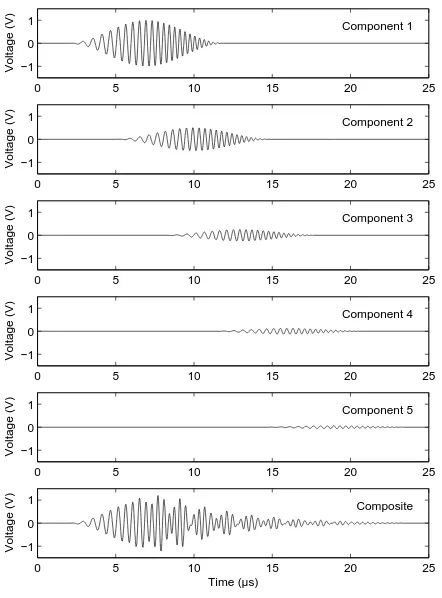
To limit the synthetic signal’s duration, the summation is performed on the first five component LFM signals (i=5). As the magnitude of the individual components decays, their effect becomes negligible. The five component LFM signals and the composite signal are shown in figure 1.
Figure 2 shows the spectra of the five individual com-ponent LFM signals and that of the composite signal after Fourier transformation. The individual component signals have a smooth spectra due to the application of Hann window and decaying maximum magnitude. The spectrum of the composite signal is not smooth as the frequency-phase relationship of the individual component signals is incoherent causing periodic constructive and destructive interference.
0 5 10 15 20 25 −1
0
1 Component 1
Voltage (V)
0 5 10 15 20 25
−1 0
1 Component 2
Voltage (V)
0 5 10 15 20 25
−1 0
1 Component 3
Voltage (V)
0 5 10 15 20 25
−1 0
1 Component 4
Voltage (V)
0 5 10 15 20 25
−1 0
1 Component 5
Voltage (V)
0 5 10 15 20 25
−1 0
1 Composite
Time (µs)
[image:4.612.322.544.62.239.2]Voltage (V)
Fig. 1. Construction of synthetic ultrasound signal through the summation of five LFM signals overlapping in the time domain
III. THEFRACTIONALFOURIERTRANSFORM
In 1980 Namias described the fractional Fourier Transform (FrFT) in its incomplete form [6], the FrFT being a general-isation of the Fourier Transform (FT). In 1987 McBride and Kerr published an extended analysis of FrFT [7] upon which most recent work is based. Whereas the conventional Fourier transform allows signals in the time domain to be transformed to the frequency domain and vice versa, the fractional Fourier transform allows signals to be transformed into a fractional domain. A fractional domain is neither time nor frequency but an intermediate domain between both time and frequency domains.
The Fourier transform is expressed as
X(f) =
Z ∞
−∞
B(f,t)x(t)dt (7)
whereB(f,t)is the transform kernel,
B(f,t) =exp(−j2πf t), (8)
and t is time and f is frequency. The FrFT is defined by modifying the Fourier transform kernel to the form [7], [8]
Bϕ(x,y)=Aϕexp
jπ x2cot(ϕ)−2xycsc(ϕ) +y2cot(ϕ)
(9)
0 1 2 3 4 5
0 0.2 0.4 0.6 0.8 1 1.2 1.4 1.6 1.8 2
Frequency (MHz)
Magnitude (AU)
Component 1 Component 2 Component 3 Component 4 Component 5 Composite
Fig. 2. Spectra of individual component LFM signals and composite signal
where
Aϕ=|sin(ϕ)|
1 2 exp
−
jπsgn(sin(ϕ))
4 +j
ϕ
2
(10)
wherexandydefine the axes of the fractional domain. Rather than defining the fraction of the transform as an angle,ϕ, in the interval [−π,π] radians, a new variable,α, is defined as the order of the transform, is valid in the interval [-2, 2] and is defined as
α=2ϕ
π . (11)
Certain transform orders are particularly noteworthy as the results of the fractional transform are identical to mathematical transforms [9] commonly used by the ultrasound community and help to provide an understanding of the functionality of the FrFT. For instance, whenα is equal to 0 (ϕ=0), the result of the FrFT is the identity transform, that is, the result is identical to the time domain signal. Whenα is equal to 1 (ϕ=π2), the result of the FrFT is identical to that of the Fourier transform (FT), the frequency domain representation of the signal. When
α is equal to -1 (ϕ=−2π), the fractional transform is identical
to the inverse Fourier transform. All other transform orders are fractional and do not correspond to conventional Fourier or time transforms.
The most relevant interpretation of the FrFT to ultrasound is the clockwise rotation of the Wigner-Ville distribution of a signal, by angle ϕ, in the time-frequency plane [10], [11]. Such a rotation is illustrated in figure 3 (left) where the time-frequency plane (t−f) is rotated clockwise by angle
ϕ forming a new reference plane, (x−y). Many derivations of the relationship between the FrFT and rotations in the time-frequency plane have been published [8], [10], [12]. A practical application of the FrFT is to the pulse compression of LFM signals, specifically in medical tissue harmonic imaging [13] and radar [14].
A. Discrete time FrFT
[image:4.612.63.284.74.373.2]Fig. 3. Clockwise rotation of time-frequency plane (t−f) by angle, ϕ, through the use of the FrFT forming a new reference plane, (x−y) (left). Rotation of the time-frequency domain using the discrete FrFT indicating the centre of rotation, Nyquist frequency and unit circle defining the compact region (right)
axis with half the total duration of the time domain signal, as illustrated in figure 3 (right). Visualisation is simplified if the frequency is considered between −fN and fN where fN is
the Nyquist sampling frequency defined as half the sampling frequency, fs, rather than between 0 and fs.
As the time-frequency domain boundaries are defined and limited by the sampling frequency and total number of sam-ples, it is possible that signal energy may be rotated outside of the valid domain. As such, the signal must be compact in the time-frequency plane, that is, must contain its energy within the unit circle as defined in figure 3 (right). Signal padding or interpolation may be required to achieve a compact signal and will increase the computational power required to perform the transform.
Direct analysis in the fractional domain is complicated by the geometrical transformation constituting the FrFT trans-form. Projection of the time axis onto the fractional axis can be achieved using simple trigonometrical transformations. Due to the rotation of the time-frequency plane forming the fractional plane, time, t, is projected onto the fractional axis,x, by [15]
µα=µtcos
α π
2
, (12)
where α is the transform order. For a discrete sampled
waveform there exists an offset between the origins of the fractional and time domains that can be calculated by [9]
Mα=
bN fs
sin
α π
2
(13)
where b is the LFM start frequency and N total number of samples.
B. Digital calculation of the FrFT
To date no definitive fast implementation of the discrete FrFT is known. Authors coining the term fast FrFT are approximating the continuous FrFT using algorithms based on the fast Fourier Transform (FFT). However, these approx-imate implementations are suitable for practical application. Ozaktas [11], [16] published details of an algorithm for digital calculation of the FrFT of computational complexity
O(N logN). Computational requirements to implement this
algorithm are similar to that of the fast Fourier transform (FFT), also of computational complexity O(N logN) [17]. Hence, applications benefiting from the FrFT require minimal additional implementation cost compared to that of the FFT.
IV. SEPARATION OF OVERLAPPINGLINEARFREQUENCY
MODULATED SIGNALS USING THEFRACTIONALFOURIER
TRANSFORM
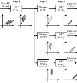
Separation of the individual LFM signals from the compos-ite signal is a three stage process:
1. A FrFT of orderαoptis performed on the composite signal
transforming the overlapping LFM signals in the time domain into separable pulses in the fractional domain. 2. The individual pulses are identified and windowed
creat-ing multiple signals each containcreat-ing one pulse.
3. The signals containing the windowed pulses are restored to the time domain using a FrFT of order −αopt thus
separating the individual LFM signals.
Each stage of the separation process is described in detail below. Figure 4 illustrates the proposed method with time-frequency plane representations of the signals at each stage of the separation process. The separation process is illustrated by the separation of the five overlapping LFM signals from the composite signal as shown in figure 1.
Fig. 4. Signal flow diagram illustrating the three stage required for separation of temporally overlapping LFM signals using the FrFT
Stage 1: Transform time domain signal using FrFT
[image:5.612.312.563.359.629.2]results in the individual LFM signals being perpendicular to the fractional axis, x, as illustrated in figure 5 (right). Under this optimal condition the projections of the LFM signals on the fractional axis are maximally separated.
Fig. 5. Rotation of Wigner-Ville distribution of three overlapping LFM signals by angleϕoptusing the FrFT to produce three non-overlapping signals
in the projection onto the fractional domain
The rate of change of frequency, d fdt, or chirp rate of the sig-nal, defines the rotation of the individual LFM signals within the time-frequency plane and hence forms the definition of the optimal rotation,ϕoptand corresponding optimal transform
order,αopt, required to maximally separate the individual LFM
signals. The optimum transform orderαopt can be defined [9]
as
αopt=−
2
πtan
−1
1 2a
(14)
wherea=B/T is the chirp rate,Bis the bandwidth in Hertz andT is the total signal duration in seconds. It should be noted that calculation of αopt only requires knowledge of the chirp
rate, a known excitation parameter. The central frequency of individual LFM signals and their location in the time domain signal is not required.
Since the input to the discrete FrFT is time sampled and hence according to Nyquist sampling theory limited in fre-quency to±fs, calculation of the optimal transform order
re-quires knowledge of the time and frequency resolution of the system,δtandδf respectively. The optimal discrete transform
order,αopt (discrete), is defined as [18]
αopt (discrete)=−
2
πtan
−1
δf/δt
2a
(15)
whereδf=fs/N andδt=1/fs, therefore
αopt (discrete)=−
2
πtan
−1
f2
s/N
2a
(16)
where fs is the sampling frequency in Hertz, N is the total
number of time samples in waveform and a is the chirp rate. The proposed method is applied to the composite signal described in II-A. The LFM signals have a bandwidth, B, of 2.5 MHz and duration, D, of 10 µs. The composite signal
has a sampling frequency, fs, of 100 MHz and total duration
of 25 µs, hence the total number of samples, N, is 2500. Using (16) the optimal transform order for the composite LFM signals is calculated asαopt=−0.9841. The FrFT is performed
in Matlab using the algorithm of Ozaktas [11], [16].
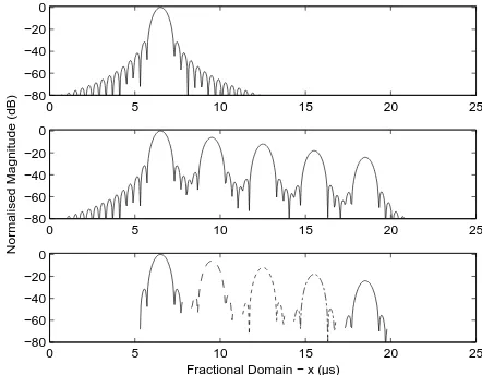
Figure 6 (top) shows the first component LFM signal, as defined by (5), after applying the FrFT transformation of op-timal order (αopt=−0.9841). Like the FFT, the output of the
FrFT is complex. In the fractional domain, the magnitude (and phase) of the signal should be examined rather than the real and imaginary data. To aid interpretation, time has been pro-jected onto the the fractional axis using (12) and (13).
Applying the FrFT transform of optimal order,αopt, to an
LFM signal maximally compresses the signal in the fractional domain, where a mainlobe and sidelobes with decaying mag-nitude are found. This illustrates the use of the FrFT for pulse compression of LFM signals.
Stage 2: Windowing in the fractional domain
The composite signal, after applying the FrFT of optimal order, is shown in figure 6 (middle). Although the mainlobe associated with each component LFM signal is clearly visible, they are in fact superimposed with the sidelobes from adjacent signals.
In order to perform separation of the LFM signals, a rect-angular window is placed around each mainlobe and the com-posite signal split into five signals. The width of the window has been optimised so that energy from a single signal is max-imised whilst minimising the energy from adjacent signals. In this simulation the width of the rectangular window is the same as the separation of the LFM signals, centred on the mainlobe. Figure 6 (bottom) shows the composite signal, in the optimum fractional domain, split into five individual signals.
Rectangular windowing is used so that the energy distri-bution of the composite signal is maintained when individual signals are created. It is also possible to use a Tukey [19] (tapered cosine) window withα, the tapering coefficient, such
that the amplitude of the mainlobe is undistorted. The use of windows which distort the amplitude of the mainlobe, for example Hann, Blackman-Harris or Gaussian windows, would introduce significant signal distortion in the time, frequency or fraction domains.
0 5 10 15 20 25
−80 −60 −40 −20 0
0 5 10 15 20 25
−80 −60 −40 −20 0
Normalised Magnitude (dB)
0 5 10 15 20 25
−80 −60 −40 −20 0
Fractional Domain − x (µs)
Fig. 6. First component LFM signal (i=1) (top) and composite signal (mid-dle) after transformation into the optimal fractional domain (αopt=−0.9841).
[image:6.612.322.543.522.694.2]Stage 3: Restore windowed signal to time domain
The individual windowed signals in the fractional domain are restored to the time domain using the inverse FrFT (iFrFT), a FrFT transformation of order −αopt, resulting in separation
of the individual component LFM signals. The output of the proposed separation method process, s(t), can be described mathematically as
s(t) =F−αopt w Fαopt(e(t))
(17)
where Fαopt is the optimal fractional transform, w(x), is the
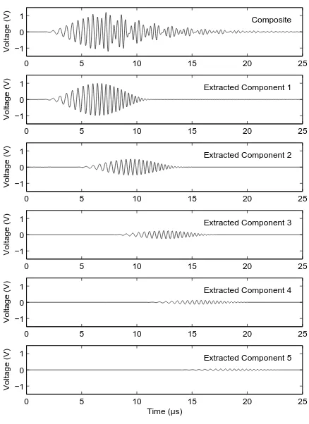
window in the fractional domain and e(t)is the input signal. The original composite signal created in section II-A and the individual LFM signals after separation by the proposed method are shown in figure 7. Comparison of the separated LFM signals with the original component signals in the time domain shows successful extraction. The separated signals are not shifted in phase and have a maximum amplitude error of ±0.6% compared to the original component signals. The spectra of the separated LFM signals are shown in figure 8 along with summation of the spectra of all the separated signals. The summation of the separated spectra is free from constructive and destructive interference present in that of figure 2. Figure 9 shows the percentage error between the spectra of the original component LFM signals and the sepa-rated signals, showing a maximum spectral error of ±0.6% is achieved using the proposed separation method. These small errors occur in the time and frequency domains and have two potential sources, both of which will distort the extracted signals. Firstly, windowing in the fractional domain cannot include the entire sidebands of the signal. Secondly, upon windowing a signal in the fractional domain, the sidebands of other signals are also windowed.
V. EXPERIMENTALINVESTIGATION
Synthetic signals are useful to assess the potential of the FrFT. Experimental validation has been performed to ensure that the effects of excitation and receiver circuitry, transducer and wave propagation on the ultrasonic signal do not severely impact the FrFT performance. The results from two experi-mental investigations are presented to assess the application of FrFT based LFM signal separation to non-invasive industrial measurement.
A. Experimental Setup
In the first investigation, a 6 mm, 304 grade stainless steel plate was placed in a water bath with a pitch catch transducer configuration for transmission measurements as illustrated in figure 10. This setup could be found in the immersion testing of metal components. Transmission of a single ultrasonic wave through the plate will result in the formation of a series of echoes with decaying magnitude, separated by the round trip time of the metal plate.
The immersion transducers used were model V323 man-ufactured by Olympus NDT with a central frequency of 2.25 MHz and fractional bandwidth of 55%. A custom linear frequency modulated excitation circuit [20] was used. The
0 5 10 15 20 25
−1 0
1 Composite
Voltage (V)
0 5 10 15 20 25
−1 0
1 Extracted Component 1
Voltage (V)
0 5 10 15 20 25
−1 0
1 Extracted Component 2
Voltage (V)
0 5 10 15 20 25
−1 0
1 Extracted Component 3
Voltage (V)
0 5 10 15 20 25
−1 0
1 Extracted Component 4
Voltage (V)
0 5 10 15 20 25
−1 0
1 Extracted Component 5
Voltage (V)
[image:7.612.326.545.73.374.2]Time (µs)
Fig. 7. Simulated ultrasound signal (top) and five component LFM signals extracted using the FrFT based method
0 1 2 3 4 5
0 0.2 0.4 0.6 0.8 1 1.2 1.4 1.6 1.8 2
Frequency (MHz)
Magnitude (AU)
Extracted 1 Extracted 2 Extracted 3 Extracted 4 Extracted 5 Combined
Fig. 8. Spectra of individual extracted LFM signals and summation on individual spectra
excitation parameters were frequency, f0, of 2.25 MHz,
band-width, B, of 2.5 MHz, duration, D, of 10 µs and excitation
voltage, Vpk-pk of 180 V. The receiver was a LeCroy 44Xi
oscillscope, with a sampling frequency, fs of 100 MHz,
[image:7.612.324.544.446.619.2]0 0.5 1 1.5 2 2.5 3 3.5 4 4.5 5 −0.8
−0.6 −0.4 −0.2 0 0.2 0.4 0.6
FFT error (%)
Frequency (MHz)
[image:8.612.313.562.50.210.2]Extracted 1 Extracted 2 Extracted 3 Extracted 4 Extracted 5
Fig. 9. Spectral error between original and extracted LFM signals
[image:8.612.64.281.62.237.2]without amplification or buffering.
Fig. 10. Schematic representation of experimental setup for ultrasound transmission through a stainless steel plate
In the second investigation, measurements of the transmis-sion of a LFM ultrasonic signal through a water-filled steel pipe were made as illustrated in figure 11. The pipe was 5 inch nominal diameter, schedule 80, manufactured from 304 grade stainless steel. The internal diameter of the pipe was 122.2 mm and wall thickness 9.5 mm. This setup is as would be found in non-invasive measurement on pipelines. Transmission of a sin-gle ultrasonic wave through the pipe does not result in echoes with decaying magnitude. Instead, due to echoes formed in both sides of the pipe wall superimposing, the magnitude in-creases, peaks, then decays. The experimental apparatus used is identical to that described above.
B. Results and Analysis
Figure 12 (top) shows the received ultrasonic waveform af-ter transmission through the stainless steel plate. Initially, be-tween 35 and 40 µs, a LFM signal is visible. Once the echo signals are received, superimposition and interference between the overlapping echoes makes the received signal appear as a
Fig. 11. Schematic representation of experimental setup for ultrasound transmission through a stainless steel pipe
series of discrete broadband pulses rather than a long duration LFM signal. Inspection in the time domain does not allow analysis of the waveform.
Applying (16) and with knowledge of the excitation param-eters, the optimum FrFT transform order,αopt, was calculated
to be -0.844. After applying the FrFT of order αopt to the
time domain signal, the signal is maximally compressed in the fractional domain. The resulting waveform is presented in figure 12. The individual echoes are clearly visible and sep-arable in the optimum fractional domain as individual peaks with decaying magnitude. The direct transmission pulse and first five echoes were windowed and restored to the time do-main, using the inverse FrFT of optimal order. These five LFM signals are shown in figure 12. An FFT was performed on the original received signal and the five separated signals as shown in figure 13. The spectrum of the original signal has the same interference characteristics as that found in the simulated waveforms in figure 2. The extracted spectra are free from interference and have the same broadband characteristics of a single LFM signal.
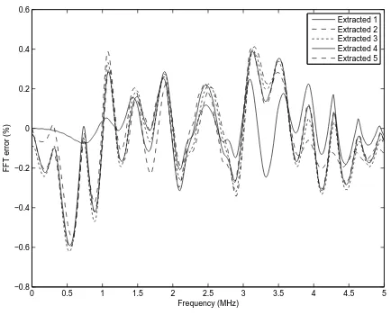
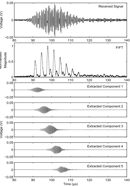
Figure 14 (top) shows the received ultrasonic waveform, consisting of overlapping direct transmission and echo signals, after transmission through the water filled stainless steel pipe. In the time domain, no individual signal component is visi-ble. As the excitation parameters remain unchanged between the two experimental investigations, the optimum transform order remains -0.844. In the optimum fractional domain the individual signals can be identified (figure 14 (middle)). Due to the change in experimental geometry and the presence of two pipe walls, each generating echoes which in turn super-impose, the pulse magnitude initially increases before peaking and decaying. After windowing in the fractional domain the individual signals are restored to the time domain as shown in figure 14 (bottom). The spectra of the direct transmission signal and individual echoes are shown in figure 15 and do not show interference.
VI. CONCLUSIONS
[image:8.612.50.301.306.471.2]30 35 40 45 50 55 60 65 70 −0.5
0 0.5
Received Signal
Voltage (V)
30 35 40 45 50 55 60 65 70
0 0.5 1
Normalised Magnitude
FrFT
−0.5 0 0.5
Extracted Component 1
−0.5 0 0.5
Extracted Component 2
−0.5 0 0.5
Extracted Component 3
Voltage (V)
−0.5 0 0.5
Extracted Component 4
30 35 40 45 50 55 60 65 70
−0.5 0 0.5
Extracted Component 5
[image:9.612.320.546.88.411.2]Time (µs)
Fig. 12. Received ultrasound signal after transmission through a 6 mm stainless steel plate, associated fractional Fourier transform and first five extracted ultrasound signals
0 1 2 3 4 5
0 0.5 1 1.5 2
Frequency (MHz)
Magnitude
[image:9.612.55.283.89.412.2]Received Signal Extracted 1 Extracted 2 Extracted 3 Extracted 4 Extracted 5 Combined
Fig. 13. Spectrum of received ultrasound signal after transmission through a 6 mm stainless steel plate and spectra of the first five extracted ultrasound signals
80 90 100 110 120 130 140
−0.05 0 0.05
Received Signal
Voltage (V)
80 90 100 110 120 130 140
0 0.5 1
Normalised Magnitude
FrFT
−0.05 0 0.05
Extracted Component 1
−0.05 0 0.05
Extracted Component 2
−0.05 0 0.05
Extracted Component 3
Voltage (V)
−0.05 0 0.05
Extracted Component 4
80 90 100 110 120 130 140
−0.05 0 0.05
Extracted Component 5
[image:9.612.322.543.517.692.2]Time (µs)
Fig. 14. Received ultrasound signal after transmission through a large stainless steel pipe, associated fractional Fourier transform and first five extracted ultrasound signals
0 1 2 3 4 5
0 0.05 0.1 0.15 0.2 0.25 0.3 0.35 0.4 0.45 0.5
Frequency (MHz)
Magnitude
Received Signal Extracted 1 Extracted 2 Extracted 3 Extracted 4 Extracted 5 Combined
[image:9.612.63.282.518.692.2]separation of temporally overlapping LFM ultrasound signals. Combining LFM excitation with pulse compression provides an increase in SNR at the receiver which is beneficial for ultra-sound measurements where high signal attenuation is found. LFM signals are of longer duration that pulsed signals, increas-ing the possibility of echoes temporally overlappincreas-ing. Tempo-rally overlapping LFM signals cannot be separated using con-ventional time domain windowing or frequency domain fil-tering as their spectra overlap. The FrFT allows filfil-tering to be performed spatially in the time-frequency plane thus over-coming limitations of filtering in either the time or frequency domains. Transformation of temporally overlapping LFM sig-nals with an FrFT of optimum order, as defined by the chirp rate of the LFM excitation, maximally compresses the signal in the fractional domain. Temporally overlapping signals become separated upon which windowing is performed to isolate indi-vidual signals. Depending on the application, these signals can be transformed into either the time or frequency domains for further analysis. The technique has been demonstrated using simulated temporally overlapping LFM signals. Comparing the spectra of the source signals with those of the FrFT separated signals showed a maximum magnitude error of ±0.6%.
This technique is especially suited to the analysis of ultra-sound signals created where layered structures are encountered creating temporally overlapping echoes. As such, two experi-mental investigations have shown the successful separation of temporally overlapping echoes created in immersion testing of stainless steel plates and non-invasive transmission through a water-filled stainless steel pipe. Many practical industrial applications are found such as composites analysis, non-inva-sive flow measurement, multi-phase flow imaging and spec-troscopy. This FrFT based signal separation technique shows great potential as the ability to decompose temporally overlap-ping signals will allow the development of new measurement applications.
REFERENCES
[1] M. Greenwood, J. Adamson, and J. Bamberger, “Long-path measure-ments of ultrasonic attenuation and velocity for very dilute slurries and liquids and detection of contaminates,”Ultrasonics, vol. 44, no. Supplement 1, pp. e461–e466, Dec. 2006.
[2] J. Martinsson, F. Hgglund, and J. Carlson, “Complete post-separation of overlapping ultrasonic signals by combining hard and soft modeling,”
Ultrasonics, vol. 48, no. 5, pp. 427 – 443, 2008.
[3] L. Wang, B. Xie, and S. I. Rokhlin, “Determination of embedded layer properties using adaptive time-frequency domain analysis,”The Journal of the Acoustical Society of America, vol. 111, no. 6, pp. 2644–2653, 2002.
[4] R. Demirli and J. Saniie, “Model-based estimation of ultrasonic echoes. Part I: Analysis and algorithms,”Ultrasonics, Ferroelectrics and Fre-quency Control, IEEE Transactions on, vol. 48, no. 3, pp. 787–802, May 2001.
[5] B. Boashash, Ed., Time frequency signal analysis and processing: a comprehensive reference. Amsterdam: Elsevier, 2003.
[6] V. Namias, “The Fractional Order Fourier Transform and its Application to Quantum Mechanics,”IMA J Appl Math, vol. 25, no. 3, pp. 241–265, Mar. 1980.
[7] A. C. McBride and F. H. Kerr, “On Namias’s Fractional Fourier Transforms,”IMA J Appl Math, vol. 39, no. 2, pp. 159–175, Jan. 1987. [8] H. Ozaktas, B. Barshan, D. Mendlovic, and L. Onural, “Convolution, filtering, and multiplexing in fractional Fourier domains and their relation to chirp and wavelet transforms,”J. Opt. Soc. Am. A, vol. 11, no. 2, pp. 547–, Feb. 1994.
[9] C. Capus and K. Brown, “Short-time fractional Fourier methods for the time-frequency representation of chirp signals,”J. Acoust. Soc. Am., vol. 113, no. 6, pp. 3253–3263, Jun. 2003.
[10] A. W. Lohmann, “Image rotation, Wigner rotation, and the fractional Fourier transform,”J. Opt. Soc. Am. A, vol. 10, no. 10, pp. 2181–, Oct. 1993.
[11] H. Ozaktas, Z. Zalevsky, and M. Kutay,The Fractional Fourier Trans-form: with Applications in Optics and Signal Processing. Wiley, 2001. [12] L. Almeida, “The fractional Fourier transform and time-frequency rep-resentations,”Signal Processing, IEEE Transactions on, vol. 42, no. 11, pp. 3084–3091, 1994.
[13] M. Arif, D. M. J. Cowell, and S. Freear, “Pulse compression of harmonic chirp signals using the fractional Fourier transform,” Ultrasound in Medicine & Biology, vol. In Press, Corrected Proof, 2010.
[14] O. Akay and E. Erzden, “Employing fractional autocorrelation for fast detection and sweep rate estimation of pulse compression radar waveforms,” Signal Processing, vol. 89, no. 12, pp. 2479 – 2489, 2009, special Section: Visual Information Analysis for Security. [On-line]. Available: http://www.sciencedirect.com/science/article/B6V18-4W4JDK7-4/2/662f9d642c68fa15417094092fe294be
[15] C. Capus and K. Brown, “Fractional Fourier transform of the Gaus-sian and fractional domain signal support,” Vision, Image and Signal Processing, IEE Proceedings -, vol. 150, no. 2, pp. 99–106, 2003. [16] H. Ozaktas, O. Arikan, M. Kutay, and G. Bozdagt, “Digital computation
of the fractional Fourier transform,”Signal Processing, IEEE Transac-tions on, vol. 44, no. 9, pp. 2141–2150, 1996.
[17] J. W. Cooley and J. W. Tukey, “An Algorithm for the Machine Calcula-tion of Complex Fourier Series,”Mathematics of Computation, vol. 19, no. 90, pp. 297–301, 1965.
[18] C. Capus, Y. Rzhanov, and L. Linnett, “The analysis of multiple linear chirp signals,” inTime-scale and Time-Frequency Analysis and Applications (Ref. No. 2000/019), IEE Seminar on, Y. Rzhanov, Ed., 2000, pp. 4/1–4/7.
[19] J. W. Tukey, “An introduction to the calculations of numerical spectrum analysis,” in Advanced Seminar on Spectral Analysis of Time Series, B. Harris, Ed. New York: John Wiley, 1967, pp. 25–46.
[20] D. Cowell and S. Freear, “Quinary excitation method for pulse compres-sion ultrasound measurements,”Ultrasonics, vol. 48, no. 2, pp. 98–108, Apr. 2008.
David Cowellreceived his M.Eng. degree in electronic and electrical engi-neering from the school of Electronic and Electrical Engiengi-neering at the Uni-versity of Leeds in 2004, conducting major projects in parallel computing and embedded system design. He completed his Ph.D. degree with the Ultrasound Group in 2008, conducting research into advanced coding excitation tech-niques and excitation circuit design for industrial instrumentation and medical imaging systems. During this time, he has performed extensive consultancy in instrumentation, FPGA, and high-speed digital hardware design. After work-ing as a research consultant in measurement and instrumentation, he joined the Ultrasound Group as a research Fellow. His main research is currently focused on non-invasive industrial ultrasound measurement. His other active research areas include advanced miniaturized ultrasound excitation systems with low harmonic distortion for phased array imaging, ultrasound system design, and signal processing.