A multi-layer active elastic metamaterial with tuneable and simultaneously negative mass and stiffness

promoting access to White Rose research papers

White Rose Research Online

eprints@whiterose.ac.uk

Universities of Leeds, Sheffield and York

http://eprints.whiterose.ac.uk/

This is a copy of the final published version of a paper published via gold open access

in Smart Materials and Structures.

This open access article is distributed under the terms of the Creative Commons

Attribution Licence (http://creativecommons.org/licenses/by/3.0), which permits

unrestricted use, distribution, and reproduction in any medium, provided the

original work is properly cited.

White Rose Research Online URL for this paper:

http://eprints.whiterose.ac.uk/79762

Published paper

This content has been downloaded from IOPscience. Please scroll down to see the full text.

Download details:

IP Address: 143.167.33.230

This content was downloaded on 11/07/2014 at 12:41

Please note that terms and conditions apply.

A multi-layer active elastic metamaterial with tuneable and simultaneously negative mass and

stiffness

View the table of contents for this issue, or go to the journal homepage for more 2014 Smart Mater. Struct. 23 075020

(http://iopscience.iop.org/0964-1726/23/7/075020)

A multi-layer active elastic metamaterial with

tuneable and simultaneously negative mass

and stiffness

S A Pope and H Laalej

Department of Automatic Control and Systems Engineering, University of Sheffield, Mappin Street, Sheffield S1 3JD, UK

E-mail:s.a.pope@sheffield.ac.uk

Received 5 March 2014, revised 26 April 2014 Accepted for publication 11 May 2014 Published 12 June 2014

Abstract

All conventional acoustic/elastic media are restricted to possess positive constants for their constitutive parameters (density and modulus). Metamaterials provide an approach through which this restriction can be broken. By making these parameters negative and/or tuneable a broader range of properties becomes possible. This paper describes thefirst experimental implementation of an acoustic/elastic metamaterial in which the material parameters can be both simultaneously negative in afinite frequency band and the magnitude of the parameters independently tuneable on demand. The design is an active metamaterial (meta-mechanical-system) which is realized by directly applying feedback control forces to each layer within the metamaterial. The ability to tune the magnitude of the negative parameters has important implications for the use of a standard design that can be tuned to a particular application, or one which can adapt to a changing performance requirement. The implementation of the design is relatively large scale and low frequency, but the unit-cell length is significantly smaller than the wavelength in the double negative band. Importantly, assuming appropriate control hardware is available, the design can be both reduced in scaled and expanded to greater degrees of freedom.

S Online supplementary data available fromstacks.iop.org/sms/23/075020/mmedia

Keywords: metamaterial, active control, density, bulk modulus, experiment

(Somefigures may appear in colour only in the online journal)

1. Introduction

Metamaterials are artificially structured periodic media which can be designed to produce an effective homogeneous response which breaks the restrictions imposed by conven-tional media. Early work conducted in electromagnetics/ optics, led to metamaterial designs in which the material parameters (permittivity and permeability) can be negative and a function of frequency (Pendryet al1996,1999, Smith

et al 2000). For a material with a simultaneously double

negative response (negative permittivity and permeability),

‘exotic’material properties arise, such as a negative refractive index and frequency dependent wave velocity (Vese-lago1968). A negative refractive index has been subsequently shown to be required for the construction of innovative devices such as invisibility cloaks (Pendry et al 2006) and sub-wavelength super lenses (Pendry 2000). Later work in other domains, such as mechanical/elastic/acoustic materials, where the parameters are the density and various elastic moduli, has yielded similar results (Li and Chan 2004, Liu

et al 2005, Wang et al 2006, Fang et al 2006) and the associated applications of invisibility cloaks (Milton

et al2006) and sub-wavelength lenses (Guenneauet al2007). In an acoustic metamaterial the propagating wave is a pres-sure wave in afluid, whereas with elastic metamaterials the

0964-1726/14/075020+11$33.00 1 © 2014 IOP Publishing Ltd Printed in the UK Smart Materials and Structures

Smart Mater. Struct.23(2014) 075020 (11pp) doi:10.1088/0964-1726/23/7/075020

Content from this work may be used under the terms of the

propagating wave can include pressure, shear or surface waves in a solid. However, there are a limited number of experimental demonstrations of acoustic metamaterials (materials in which the density and bulk modulus are the focus) which possess a frequency band with a simultaneously double negative response. Thefirst double negative acoustic metamaterial consisted of a one-dimensional tubefilled with air in which side holes are drilled and separated internally by membranes (Leeet al 2010). A second design used a com-bination of split hollow spheres and hollow rods to create a double negative response in a narrow bandwidth (Chen

et al 2013). This double negative acoustic metamaterial is described as three dimensional. However, in reality its novel response is present in two dimension and tested in one dimension using an impedance tube, whereas it is the con-struction that is three dimensional. Subsequent work showed the negative refractive behavior of the metamaterial in two dimensions (Zhaiet al 2013). A third design uses a ‘ space-coiled’metamaterial in which the incident wave is forced to follow a pre-defined path within a unit-cell (Xieet al2013). A potential problem with this design is the considerable extra distance that the wave has to travel within the unit-cellcom-pared to free space. This potentially increases the losses and the phase difference of the manipulated wave compared to a wave in free space, which can be an issue in cloaking applications. Experiments were conducted for a two dimen-sional arrangement of units cells, which showed a negative refractive index. However, the negative effective parameters were only measured for a single discrete unit cell and the bulk property of the metamaterial was inferred from these mea-surements. The lack of experimental demonstrations of dou-ble negative acoustic or elastic metamaterials is in despite some properties, such as larger wavelengths compared to electromagnetic applications, removing the need for micro or nano-fabrication in some cases, which leads to a more amenable design prospect. However, in contrast the full elastodynamic wave equation leads to a more complex response requiring both pressure and shear wave effects to be designed for and as yet elastic metamaterials that do this have not been manufactured. In-fact all experimental double negative metamaterials have focused on pressure waves. No experiments of negative density and shear modulus meta-materials have been presented. The importance of developing the field of metamaterials in domains other than electro-magnetics has been recently highlighted (Wegener 2013). One particularly promising route is the potential of active acoustic (AAM) and active elastic (AEM) metamaterials. Active digital control provides the potential to realize designs which are not possible with passive components alone, have a wide range of parameter values and which are tuneable almost instantly on demand. Other proposed tuneable designs rely on soft media (Brunet et al2013), which can limit their use to applications with low load bearing requirements, or require changes in constituent media to implement the tuning (Liang

et al2012), which does not allow the design to be tuned easily

in situ. Compared to electromagnetic applications, the con-siderably lower frequency of most noise and vibration applications brings digital active control well within the

boundaries of current technology. For example, the visible light spectrum is about 430–790 THz, requiring extremely high sample rates. In contrast, the audible frequency spectrum is about 20 Hz–20 kHz, which is well within the reach of current digital electronics. For this reason electromagnetic/ optical active metamaterials have relied on other designs (Boardmanet al2011), which do not necessarily possess the

flexibility associated with digital control.

A theoretical design for a one-dimensional AEM with both mass and in-plane stiffness which can become simulta-neously negative and tuneable across a designed frequency band has been previously proposed (Pope and Daley 2010, Pope et al 2012). These designs were based on a series of actively controlled resonators connected to a viscoelastic transmission system. Recently a design for a one-dimensional AAM which has a positive bulk modulus and a density response which is negative and tuneable across a designed frequency band was experimentally demonstrated for a single layer (unit cell) (Popaet al2013). Other related work includes a design for a theoretical one-dimensional AAM in which both the density and bulk modulus can be simultaneously tuned to a wide range of positive values across a frequency range (Akl and Baz 2013). These designs are based on actively controlled periodic membranes and Helmholtz reso-nators. Other work has proposed theoretical designs for acoustic lenses based on AAMs (Wen et al2013).

This paper presents the experimental implementation and characterization of the previously proposed double negative AEM (Pope and Daley 2010, Popeet al 2012). As with the previous passive double negative acoustic metamaterials (Lee

et al2010, Chenet al2013) the design is tested using a one-dimensional setup, which is sufficient to provide proof of principle. However, unlike the previous passive designs, the paper shows how the feedback control system can be used to tune the magnitude of the negative parameters on demand. This has important implications for the use of metamaterials in applications which need to adapt to a changing environ-mental or user scenario. In addition, the double negative frequency band is located at approximately 30 Hz, which is at least an order of magnitude below what has been achieved with the previous passive designs. The location of this fre-quency band places it within the domain applicable to seismic and civil applications.

2. AEM—theory

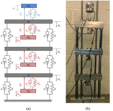
The AEM infigure1(a) consists of several layers (unit cells). Each layer is composed of a pair of masses m connected together by linear springs k and dashpot dampers c in the Kelvin–Voigt arrangement for viscoelasticity. This is the

transmission system (Pope and Daley2010). This system was shown to theoretically possess a double negative (negative mass and stiffness) frequency band when subjected to a pre-designed feedback control force. The AEM infigure 1(a) is almost identical to the earlier theoretical design, with the inertial mass of the actuator replacing the locally resonant masses. The only difference is that in this system the active force acts across the actuator, such that it is applied to the transmission mass and with inverse phase to the inertial mass. The effects of using an inertial actuator on the theoretical performance and stability of an AEM has previously been investigated (Popeet al2012). One important benefit of using an inertial actuator is that because it does not require afixed termination, the control force is effectively embedded locally within the material.

Three masses are sufficient to demonstrate that negative effective parameters have been achieved and the response is homogeneous over multiple unit cells. More cells can be added, but little is gained in terms of knowledge. Even though this is a single dimension design and any propagating wave is constrained to be in-plane pressure variations, the concept can

be generalized to higher dimension and for both pressure and shear waves. With this design the onlyfixed connection point is between the bottom mass and the base. This is an important addition to the design and experiment. The previous experi-ments using double negative passive acoustic metamaterials have assumed a free boundary condition and thus no static load bearing capability. The design here explicitly includes a

fixed boundary point, allowing the metamaterial to be load bearing. In addition, many practical applications of metama-terials (such as an invisibility cloak attached to and sur-rounding an object) will also inherently require metamaterials to exhibit their desired response when integrated into an arrangement with afixed boundary.

The equations of motion of the three transmission masses are (1a)–(1c). f=f_d +c ud

(

˙ − ˙d u1

)

+kd(ud− u1)is the total

disturbance force applied by the disturbance actuator

¨ = ˙ − ˙ + −

+

(

˙ − ˙

)

+ − + −

(

)

mu c u u k u u

c u u k u u f f a

2 2 ( )

( ) (1 )

a a a a

1 2 1 2 1

1 1 1

1 1

[image:5.595.109.496.69.449.2]

Smart Mater. Struct.23(2014) 075020 S A Pope and H Laalej

Figure 1.The active elastic metamaterial. (a) Is the theoretical design in which the elements with no subscript indicate the transmission system, elements labeled with the subscript a the control actuator components and elements with the subscript d the disturbance actuator components. (b) is the experimental implementation, which is aligned with the theoretical design in (a) for ease of comparison.

¨ = ˙ + ˙ − ˙ + + −

+

(

˙ − ˙

)

+ − −

(

)

(

)

mu c u u u k u u u

c u u k u u f b

2 2 2 2

( ) (1 )

a a a a

2 1 3 1 1 3 2

2 2 2

2 2

¨ = ˙ − ˙ + −

+

(

˙ − ˙

)

+ − −

(

)

(

)

mu c u u k u u

c u u k u u f c

2 2 2 2

( ) . (1 )

a a a a

3 2 3 2 3

3 3 3

3 3

The equations of motion of the three inertial actuators are (2a)–(2c)

¨ =

(

˙ − ˙

)

+ − +

m ua a1 c ua 1 ua1 ka(u1 ua1) f1 (2 )a

¨ =

(

˙ − ˙

)

+ − +

m ua a2 c ua 2 ua2 ka(u2 ua2) f2 (2 )b

¨ =

(

˙ − ˙

)

+ − +

m ua a3 c ua 3 ua3 ka(u3 ua3) f3. (2 )c

Converting into a frequency domain form of the equations of motion, and substituting for the motion of the inertial masses from (2a)–(2c) into (1a)–(1c), leads to (3a)–(3c) and (4).U_n,F_nand Fare the harmonic form of the variables u_n, f_n and f. The passive resonance of the inertial actuator leads to an initial frequency dependent form for the effective stiffnessm_p

( )

jω , which will be further modified by the feedback control force f

n

ω ω ω

ω ω ω − = + − + + − + +

( )

(

) (

)

m i U c i k U U F

m

m c i k F a

2

(3 ) p

a

a a a

2

1 2 1

2

2 1

ω ω ω

ω ω ω − = + + − + − + +

( )

(

) (

)

m i U c i k U U U

m

m c i k F b

2 2

(3 ) p

a

a a a

2

2 1 3 2

2

2 2

ω ω ω

ω ω ω − = + − + − + +

( )

(

) (

)

m i U c i k U U

m

m c i k F c

2 2

(3 ) p

a

a a a

2

3 2 3

2 2 3 ω ω ω ω = + + − + +

( )

(

)

m i m m c i k

m c i k . (4)

p

a a a

a a a

2

The feedback control force can be divided into a part designed to control the effective mass of the system and a part designed to control the effective stiffness, such that

= +

f_n f_n f_n

m k. The aim is to select the control forces so that

each of equations (3a)–(3c) can be written in the form for an homogeneous effective system in which each equation of motion has the same effective mass and stiffness function. For the effective mass this is straightforward to achieve using a collocated control system that feeds back the acceleration of each local transmission mass, such that f_n = −m u_c¨_n

m , where

m_c is the control parameter. This leads to the three frequency domain control forces (5a)–(5c)

ω

=

F1 mc U (5 )a

2 1 m

ω

=

F2 mc U (5 )b

2 2 m

ω

=

F3 mc U. (5 )c

2 3 m

For the effective stiffness the motion of the adjacent transmission masses need to be included in the control force. For an infinite number of transmission masses this leads to the non-collocated feedback force fn_k = k uc

(

n−1+un+1− 2un

)

,

in whichk_c is the control parameter. The use of the feedback control system allows the boundary conditions to be explicitly taken into consideration to maintain the homogeneous struc-ture. This is important for the stiffness control force f

nk since

it inherently includes the motion of the connections either side of each transmission mass. The three stiffness control forces that take into account the free boundary for the top mass and the zero motion of the fixed boundary (point four) at the bottom mass are (6a)–(6c). By comparison of (6a)–(6c) with (3a)–(3c), it is clear that the displacements in each of the stiffness control forces are chosen so that the feedback signal can combine with the passive equivalent stiffness c iω +k, i.e. the stiffness control system emulates the connections required to influence the effective stiffness of the system

=

₍

−

₎

F1k kc U2 U1 (6 )a

=

(

+ −

)

F2k kc U1 U3 2U2 (6 )b

=

₍

−

₎

F3k kc U2 2U3 . (6 )c

On substitution of the control forces (5a)–(5a) and (6a)–(6c) into (3a)–(3c), the homogeneous effective system of (7a)–(7c) is realized, in which the effective mass (8) and the effective stiffness (9) are both complex functions of frequency and independently controlled by m_c andk_c respectively. The real parts of the mass (8) and stiffness (9) determine the wave propagation characteristics such as phase velocity in the effective medium. The imaginary parts constitute the losses in the effective medium

ω ω ω

−m ie

( )

U =k ie

( ) (

U −U

)

+F (7 )a

2

1 2 1

ω ω ω

−m ie

_{( )}

U =k ie

_{( ) (}

U +U −2U

₎

(7 )b

2

2 1 3 2

ω ω ω

−m ie

( )

U =k ie

( ) (

U −2U

)

(7 )c

2

3 2 3

ω ω ω

ω ω

= + + +

− + +

(

)

( )

m i m m m c i k

m c i k (8)

e

a c a a

a a a

2

2

ω ω ω

ω ω

= + +

− + +

( )

(

)

k i c i k m k

m c i k

2 . (9)

e

a c

a a a

2

2

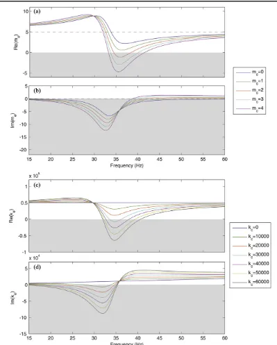
The simulated response of the effective mass and stiffness for a range of feedback gains is plotted infigure 2. The para-meters for the simulation are taken to match the identified parameters of the experimental implementation shown in

figure1(b). The experimental system is described in more detail in the next section. These simulated effective parameters include the electrical characteristics of the voice-coil in the control actuators. This can be modeled by an inductanceL_a, resistorR_a

mass (10) and stiffness (11). g

ea and gma are the gains for the

voice-coil and driver amplifier respectively. The explicit deriva-tion of (10) and (11) is included in the supplementary material (available atstacks.iop.org/SMS/23/075020/mmedia).

ω

ω ω ω ω

ω ω ω ω

=

+

+ + + +

− + + + +

(

)

(

)

( )

(

) (

)

(

)

m i

m

m m g g g i c i k L i R

m c i k L i R g i (10)

e

a c e m e a a a a

a a a a a e

2 2

2 2

a a a

a

ω ω

ω

ω ω ω ω

= +

+

− + + + +

(

)

( )

(

)

(

)

k i c i k

m k g g

m c i k L i R g i

2

. (11) e

a c e m

a a a a a e

2

2 2

a a

a

Both the effective mass and stiffness contain a resonance at 30 Hz which is associated with the mechanical components of the actuator and can be independently controlled through the feedback gains m_c andk_c respectively. The effect of this resonance is to amplify the feedback control forces in the

[image:7.595.97.496.61.558.2]

Smart Mater. Struct.23(2014) 075020 S A Pope and H Laalej

Figure 2.The frequency response of the simulated material parameters of the effective system representation of the active elastic metamaterial. (a) and (c) are the real part effective mass and stiffness respectively of the simulated system when the feedback back gains are

=

[

]

mc 0, 4 andkc=

[

0, 60 000

]

. (b) and (d) are the imaginary parts of the effective mass and stiffness respectively. The grey regions mark

the negative domain. The dashed black lines in (a) and (b) are the parameters for the transmission system (the system without any actuators attached), which for the stiffness of the simulated system is the same as whenkc=0.

region immediately above the resonant frequency. The effect of the resonance on the control forces can be seen by the resonant transfer function in each of the terms on the right-hand side of (3a)–(3c). The polarity of the feedback signal is such that the real parts of the effective parameters can be driven negative in this frequency region for sufficiently large feedback gains. As the feedback gains are increased the magnitude of the parameters in the negative band increase. Another way of viewing the system is that, in this frequency region f_n

m causes the acceleration of each transmission mass

to exhibit a dipole resonance which is out of phase with a driving force and f

nkcauses the relative displacement response

of two adjacent transmission masses to exhibit a monopole resonance which is out of phase with a driving force. The effective mass control force f_n

m contains only the local

acceleration of each transmission mass. Thus it adds to the effect of the local dipole resonance created by the passive mechanical components of the inertial actuators, which is the dispersive part of (4). The choice of feedback displacements for the effective stiffness control forces f

nk in (6a)–(6c)

include the motion of the adjacent masses. This ‘virtual’ connection essentially converts the local actuator resonance into a response that emulates a monopole resonance, allowing the effective stiffness to be controlled.

3. AEM—experiment

Figure1(b) shows a photograph of the experimental imple-mentation of the proposed AEM. It is constrained to move in a single dimension by two vertical metal bars which pass through linear bearings integrated into each of the aluminum transmission masses. It is mounted vertically to reduce the load on the bearings and thus minimize the losses associated with them. The connecting springs are steel coils. The control actuators are of the electromagnetic voice-coil type (Data Physics Corporation IV40) and each has a mechanical reso-nance of 30 Hz, which is above the largest of the three natural frequencies of the transmission system. These actuators are chosen due to their well-defined characteristics and easily modelled performance. The motion of each mass is measured by an accelerometer (PCB Piezotronics 333B50) which is connected to a digital data acquisition and control unit (dSPACE control unit). This same unit also closes the loop and provides the control force in the form of a voltage to each of the actuators through amplifiers (Data Physics Corpora-tion). The disturbance (external) force is applied to the top mass by another inertial actuator (Data Physics Corporation IV45). The total disturbance force, which is the sum of the force provided by the electromagnetic component of the actuator and the resonance force associated with the relative motion of the inertial mass of the actuator and the top transmission mass, is directly measured by a load cell (Novatech F256). The digital control unit is set to sample at a rate of 2 kHz, which is sufficient to extract the relevant fre-quency data and minimize the inherent delay in the feedback

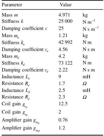
loops. The actuators and sensors have been chosen based on the availability of suitable commercial off-the-shelf compo-nents. Importantly, since the novel characteristics are not a function of the dimensions of the sub-systems, the general concept is scalable through the use of different transmission components and sensor and actuator technology. For exam-ple, the current separation between two adjacent transmission masses is approximately 300 mm. This is larger than the 70 mm unit cell length in the first double negative passive acoustic metamaterial (Leeet al2010). However, the unit cell size in this AEM was limited by the length of the transmission springs with the required stiffness. The length of the control actuator is 75 mm and this (plus a small distance to allow for its motion and connection) provides the minimum gap pos-sible between the transmission masses. Thus with shorter springs the unit cell can be reduced to a length comparable to the first double negative acoustic metamaterial. The para-meters of the experimental AEM have been determined through either direct measurement (e.g. mass), manufacturers supplied values or through fitting a model to the component or systems response. These parameters are listed in table 1

and are similar to those used in previous theoretical and simulated work (Pope et al2012).

[image:8.595.335.518.93.332.2]

The general concept of the system in figure 1 can be described as a mechanical metamaterial since the objective is to emulate the response of a material with certain effective non-conventional parameters. However the term meta-mechanical-system is probably a more accurate description for a number of reasons. Firstly, the term meta-mechanical-system acknowledges that the proposed design is more than a material composed of an array of passive meta-atomʼs, but is instead a system composed of an array of sub-systems that can incorporate embedded sensors, actuators and feedback Table 1.Material and component parameters identified for the experimental AEM.

Parameter Value

Massm 4.971 kg

Stiffnessk 25 000 −

N m 1

Damping coefficientc 25 −

N s m 1

Massma 1.21 kg

Stiffnessk_a 42 992 N m

Damping coefficientca 4.56 N s m

Massmd 4.2 kg

Stiffnessk_d 73 122 N m

Damping coefficientcd 2.22 N s m

InductanceL_a 9 mH

ResistanceRa 1.7 Ω

InductanceL_d 2.5 mH

ResistanceRd 2.3 Ω

Coil gaing_e

a 12.5

Coil gaing_e

d 2

Amplifier gaing_m

a 0.76

Amplifier gaing_m

loops that may lead to some form of inter-connection between the separate sub-systems. Secondly, the lumped element experimental realization in figure 1(b) does not posses the homogeneous bulk composition associated with a material, despite it being possible to extend the design to a homo-geneous material with embedded sensors and actuators, which would effectively provide the same response.

A crucial stage in the experimental analysis of double negative elastic metamaterials is extracting the negative effective parameters. In previous studies, two different approaches have been used. In thefirst experiment conducted using a double negative acoustic metamaterial, the sign of the effective density was measured by comparing the phase dif-ference between the pressure gradient in adjacent unit cells and the displacement of the membrane separating the two cells (Lee et al 2010). Opposing phase indicates negative density. However, this method does not provide an actual value for the density, just its sign. In contrast the sign of the negative bulk modulus was not measured directly. The phase velocity was measured by observation of the time series of the pressure measurements in the unit cells. This was possible due to the use of a matched boundary condition that elimi-nated any reflection at the boundary, leading to a bulk wave propagating in a single direction in the effective medium. A negative bulk modulus was then inferred from the simulta-neous observation of both a negative phase velocity and negative density. Later work used a method requiring mea-surements of the reflection and transmission coefficients of the acoustic metamaterial (Fokinet al2007, Chenet al2013, Xie et al 2013). The method assumes a plane wave dis-turbance that is normal to the boundary of the metamaterial. In this form it is only suitable for extraction of effective density and bulk modulus (not shear modulus or density when the system is subjected to a shear wave excitation) of one dimensional materials. Due to multiple possible solutions, it makes several more assumptions required to calculate the correct signs for the effective parameters from the impedance and refractive index, which are derived from the reflection and transmission coefficients. Importantly, one of these assumptions is that the metamaterial is passive, leading to a positive imaginary part of the impedance due to the inherent dissipation. Since this assumption does not necessarily hold for active metamaterials, the correct signs cannot always be extracted.

Neither of the two previous approaches to effective parameter extraction can be directly used for the metamaterial implemented in this study, because it includes a fixed boundary and is actively controlled. In this paper a derivative of well-known gray box systems identification techniques are used to identify the parameters of a model for the effective system. The advantage of this method is that it is not restricted to passive systems and it can be applied to systems with arbitrary boundary and wave propagation, assuming that the correct initial model structure is known. Since the experiment is constrained to pressure waves in a single dimension, the assumed effective model is that of the standard lumped element form of the one dimension pressure wave equation. Analysis of the direct measurements of the motion

of the internal structure of the metamaterial, together with the analysis of the model residuals, allows additional information to be extracted, such as the presence of any inhomogeneity. By extension to a full black box identification routine, the method could also be used to extract the explicit structure for the model, as opposed to making an initial assumption about its structure, as is the case with the grey box approach used here.

The method used to identify the parameters of the effective system description is derived as follows. The set of assumed time domain equations describing the three mass system infigure1(b) are (12a)–(12c)

¨ = − +

m ue 1 ke(u2 u1) f (12 )a

¨ =

(

+ −

)

m ue 2 k ue 1 u3 2u2 (12 )b

¨ =

(

−

)

m ue 3 k ue 2 2u3 . (12 )c

By converting to the frequency domain and re-writing (12a)–(12c) in terms of the harmonic displacements they become (13a)–(13c)

ω

−me U =k Ue

(

−U

)

+F (13 )a

2

1 2 1

ω

−me U =k Ue

(

+U −2U

)

(13 )b

2

2 1 3 2

ω

−me U =k Ue

₍

−2U

₎

. (13 )c

2

3 2 3

Since −ω2U_n= T j_n

( )

ω F (where T j_n

( )

ω is the discrete frequency transfer function between the input force and each of the acceleration measurements

(

n= 1, 2, 3

)

), (13a)–(13c) can be further reduced on substitution and cancellation to (14a)–(14c), which can be re-arranged and re-written in matrix form as (15)

ω = − ω− ω − ω +

(

)

( )

( )

( )

m T je 1 ke T j T j 1 (14 )a

2

2 1

ω = − ω−

(

ω + ω − ω

)

( )

( )

( )

( )

m T je 2 ke T j T j 2T j (14 )b

2

1 3 2

ω = − ω− ω − ω

(

)

( )

( )

( )

m T je 3 ke T j 2T j . (14 )c

2

2 3

ω ω ω

ω ω ω ω

ω ω ω

= − + − − − − − ⎡ ⎣ ⎢ ⎢ ⎤ ⎦ ⎥ ⎥ ⎡ ⎣ ⎢ ⎢ ⎢ ⎢ ⎤ ⎦ ⎥ ⎥ ⎥ ⎥ ⎡ ⎣⎢ ⎤ ⎦⎥

(

)

(

)

(

)

( )

( )

( )

( )

( )

( )

( )

T T j T j

T T j T j T j

T T j T j

m k 1 0 0 2 2 . (15) e e 1 2 2 1 2 2

1 3 2

3

2

2 3

Equation (15) is of the form y=Xβ and thus the least squares solution β=

(

X XT

)

−1XTyis readily available and can be used to calculate the complex effective mass and stiffness at discrete frequencies across the desired frequency range using the acceleration frequency response transfer functions

ω

( )

T jn determined from the experimental data. This approach

can be easily extended to any number of unit cells or higher dimension arrangements. The structure of the matrixXrelates to the configuration of the material/system. Each row corre-sponds to each degree of freedom of each transmission mass, so apelement one-dimension system would haveprows. The

first column ofXcorresponds to the effective mass, so will be the column of acceleration transfer functions. The second

Smart Mater. Struct.23(2014) 075020 S A Pope and H Laalej

column is the column of transfer functions relating to the stiffness connections in the desired effective system. For a one-dimension system ofpmasses rowsn = 2 ton=p− 1

will beω−

(

Tn−

( )

jω + Tn+

( )

jω −2T jn

( )

ω

)

2

1 1 , i.e., each mass

is connected on either side by a stiffness element. Rows 1 and

p are modified forms of this function to accommodate the boundary conditions. y is the vector of normalized magni-tudes of external forces acting on each mass in the system. For this system a single external force is present atn = 1.

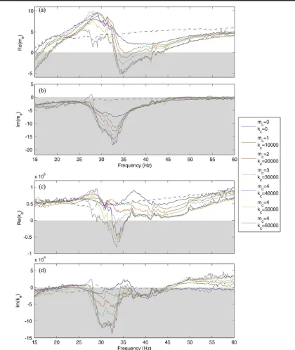
In comparison to the simulated system, the effective parameters of the experimental implementation of the AEM for the same range of feedback gains, is shownfigure3. To calculate the effective material parameters plotted infigure3, 120 s of acceleration and force input data was collected for the AEM subject to each of the pair of feedback gains. The input signal was band limited white noise. For each data set the discrete frequency transfer functionT j_n

( )

ω between the input force and each of the acceleration measurements

=

(

n 1, 2, 3

)

was calculated across the frequency domain

⎤⎦

(

0, 1 kHz at 0.1 Hz intervals. The parameters were then determined from β=

(

X XT

)

−1XTy. The residuals resulting from the parameter identification are shown infigure4, which indicates that above 30 Hz the assumption of an homo-geneous effective system is correct and the parameters are identified to a good level of accuracy.

From figure 3 the first observation is that the experi-mental results do replicate the important characteristics of the simulated results, including the overall shape and the tuneable negative behavior. As each feedback gain is increased the real part of the targeted parameter approaches and crosses zero for a critical gain in the region immediately above the control actuator resonance. Further increasing the feedback gains broadens the negative frequency band and increases the magnitude of the parameters in the negative band. The second observation is that the real part of the non-target parameter (i.e.k_eform_candm_efork_c) does also show some dependence on the feedback gain, unlike the theoretical and simulated results infigure 2. This is evident for the system response in

figure 3 in the region immediately below 30 Hz, when the mass feedback gain is fixed at mc= 4 and the stiffness

feedback gain is increased from kc=40 000 to 60 000.

However, in the double negative region the two parameters are controlled much more independently. The deviation of the response extracted from the experimental data from that of the simulation is partly due to several types of un-modeled dynamic: local losses in the bearings, springs which are not massless, a local resonance due to the bearings and variations in the actual component parameters such that they are not identical throughout the experimental system. The effect of the mass of the springs has been identified as the likely reason for the coupling between the two control regions below 30 Hz. The deviation below 21 Hz is due to the input force lying below the resonance of the disturbance actuator, which leads to a small magnitude for the input force and thus a low signal-to-noise ratio in the measured variables. A third

observation is that the effective mass matches the response of the simulated system very well above 21 Hz, whereas the effective stiffness shows more of a deviation. The most sig-nificant difference is that the stiffness returns to a positive value much quicker when compared to the simulated system, leading to a narrower negative stiffness band for the relevant feedback gains.

3.1. AEM—bandwidth analysis

The simulated data in figure2 predicts that feedback gains of mc=4 and kc=60 000 should lead to a significant

simultaneously double negative response. Fromfigure3it is clear that the simultaneously double negative response has been achieved. The real part of the mass and stiffness of the AEM subject to feedback gains of mc= 4 andkc=60 000

are plotted separately and overlaid infigure5. The effective mass is negative across the frequency range⎡⎣32.8, 41.7⎤⎦Hz and the effective stiffness negative across the frequency range ⎡⎣30.3, 35.8⎤⎦ Hz. Thus a simultaneously double

negative band exists over the frequency range⎡⎣32.8, 35.8⎤⎦

Hz. The double negative band is quite narrow (3 Hz) due to the deviation of the stiffness from the simulated systems response and the inherent locally resonant nature of the design. However, in the band the maximum magnitude of the negative parameters is substantial. The ratios of mag-nitude of the maximum negative effective parameter to transmission parameter are −1.04 for the effective mass and −1.63 for the effective stiffness, corresponding to absolute values of −5.17 kg and−81500 N m−1. The max-imum feedback gains used (mc=4 and kc=60 000)

cor-respond to close to the maximum force that can be generated by the control actuators and thus these effective material parameters represent the approximate maximum that can be achieved with this implementation. In compar-ison the passive acoustic metamaterial composed of split hollow spheres and hollow cylinders achieved a double negative bandwidth of 42 Hz, but with a lower edge of 1612 Hz and maximum negative parameters (normalized to the transmission medium) of approximately−6.5and−3.8

(Chenet al2013). The main reason for the larger bandwidth and magnitude of the parameters compared to the AEM demonstrated here is the large inherentlosses in the inertial actuators, which reduces the strength of the local resonances.

3.2. AEM—sub-wavelength analysis

For the AEM to be considered as a homogeneous material to a propagating wave, the unit cell (layer) size must be con-siderably smaller than the wavelength

( )

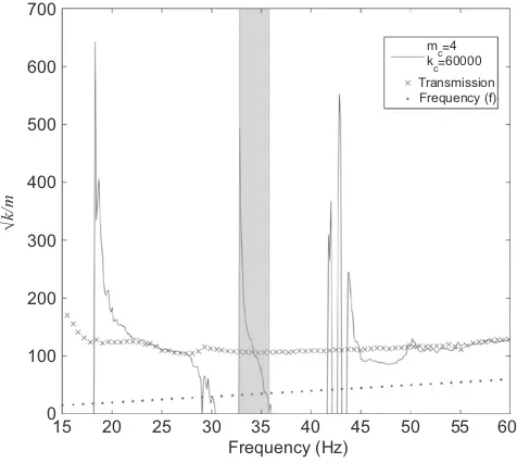
λ of the propagating wave, i.e.λ≪d, wheredis measured across the center lines of the transmission masses. For a lumped element system, such as the one adopted here, the sub-wavelength condition reduces to f≪ k m for the transmission system and

≪

( )

( )

wherefis frequency in Hz. Figure6plots both k m for the

transmission system and k f_e

( )

m f_e

( )

for the AEM when

=

mc 4andkc=60 000. The ratio for the transmission system

(crosses) is at least twice the frequency (dots), thus the required condition is met over the whole of the plotted fre-quency range. For the AEM (black line) the significant changes due to its resonant characteristics lead to several frequency bands in which the condition is met. The periods

when this line is zero correspond to when a single parameter is negative and thus the phase velocity is imaginary. The grey band marks the double negative region for the AEM. In approximately the lower half of this region the condition is met, whereas in the upper half the response approaches and crosses the frequency line. The conclusion is that in the lower half of the grey band the AEM can be considered as a homogeneous material with negative effective material parameters.

[image:11.595.88.508.62.560.2]

Smart Mater. Struct.23(2014) 075020 S A Pope and H Laalej

Figure 3.The frequency response of the experimental material parameters of the effective system representation of the active elastic metamaterial. (a) and (c) are the identified real part of the effective mass and stiffness respectively of the simulated system when the feedback back gains aremc=

[

0, 4

]

andkc=

[

0, 60 000

]

. (b) and (d) are the imaginary parts of the effective mass and stiffness respectively. The gray

regions mark the negative domain. The dashed black lines in (a) and (b) are the parameters for the transmission system (the system without any actuators attached), which for the stiffness of the simulated system is the same as whenkc=0.

4. Conclusions

[image:12.595.83.495.63.365.2]

This is thefirst time that an AEM which has simultaneously negative mass and stiffness has been experimentally demon-strated. It is also thefirst experimental implementation of an

Figure 4.The frequency response of the mean-square-error, where the errors are the real and imaginary parts of the residualsy−Xβ

[image:12.595.52.291.436.631.2]

resulting from the least-mean-square parameter identification method for the active elastic metamaterial when subjected to the seven combinations of feedback control parameters. The residuals are already normalized sincey=

[

1 0 0

]

T. The transmission system is also included and indicated by the dashed black line.

Figure 5.The frequency response of the real part of the effective mass and stiffness of experimental active elastic metamaterial when the feedback back gains aremc=4andkc=60 000. The light gray

region marks the negative domain.

k/m

700

600

500

400

300

200

100

0

15 20 25 30 35

Frequency (Hz)40 45 50 55 60

√−

−−−

m_c=4 k_c=60000 Transmission Frequency (f)

Figure 6.The frequency response of the sub-wavelength homo-geneous condition k m determined using the identified parameters for the experimental system. The red and blue lines are the sub-wavelength condition for the transmission and active elastic metamaterial (mc=4andkc=60 000) respectively. The black line

[image:12.595.311.549.437.650.2]

elastic metamaterial in which the negative parameters can be independently tuned. The work adds to the limited number of passive andfixed response acoustic/elastic metamaterials that have been demonstrated experimentally. The feedback control system is crucial to emulating the cross-coupling that is required to convert a local dipole resonance into a monopole resonance that effectively acts between two adjacent ele-ments. This result is an important milestone in creating active tuneable metamaterials for some of the previously proposed novel applications. The experimental design is composed of a lumped element test rig with integrated sensing, actuation and feedback loops. This leads to a realization of the design that can be more accurately described as a Meta-Mechanical-System, as opposed to a metamaterial, which implies more of a bulk material construction. Importantly, because the prop-erties of the metamaterial are not determined by the dimen-sions of the sub-systems, the design is scalable, assuming that suitable materials and control hardware are available. The design and experiment show that the novel properties can also be realized with a load bearing structure with a fixed boundary condition. The load bearing nature coupled with the frequency of the double negative band, which is below 50 Hz, places it in the application domain of a wide range of vibra-tion control problems, including earthquake cloaks which have previously been identified as a potential application for elastic metamaterials (Farhatet al 2009, Stenger et al 2012, Kim and Das2012).

Acknowledgments

The authors gratefully acknowledge the support of the UK Engineering and Physical Science Research Council through grant EP/J003816/1.

References

Akl W and Baz A 2013J. Vib. Acoust.135031001

Boardman A D, Grimalsky V V, Kivshar Y S, Koshevaya S V, Lapine M, Litchinitser N M, Malnev V N, Noginov M,

Rapoport Y G and Shalaev V M 2011Laser Photon. Rev.5

287–307

Brunet T, Leng J and Mondain-Monval O 2013Science342323–4

Chen H, Zeng H, Ding C, Luo C and Zhao X 2013J. Appl. Phys. 113104902

Fang N, Xi D, Xu J, Ambati M, Srituravanich W, Sun C and Zhang X 2006Nat. Mater.5452–6

Farhat M, Guenneau S and Enoch S 2009Phys. Rev. Lett.103

024301

Fokin V, Ambati M, Sun C and Zhang X 2007Phys. Rev.B76

144302

Guenneau S, Movchan A, Petursson G and Ramakrishna S A 2007

New J. Phys.9399

Kim S H and Das M P 2012Mod. Phys. Lett.B261250105

Lee S H, Park C M, Seo Y M, Wang Z G and Kim C K 2010Phys. Rev. Lett.104054301

Li J and Chan C T 2004Phys. Rev.E70055602

Liang Z, Willatzen M, Li J and Christensen J 2012Sci. Rep.2859

Liu Z Y, Chan C T and Sheng P 2005Phys. Rev.B71014103

Milton G W, Briane M and Willis J R 2006New J. Phys.8248

Pendry J B 2000Phys. Rev. Lett.853966–9

Pendry J B, Holden A J, Robbins D J and Stewart W J 1999IEEE Trans. Microw. Theory472075–84

Pendry J B, Holden A J, Stewart W J and Youngs I 1996Phys. Rev. Lett.764773–6

Pendry J B, Schurig D and Smith D R 2006Science3121780–2

Popa B I, Zigoneanu L and Cummer S A 2013Phys. Rev.B88

024303

Pope S A 2013IEEE Trans. Ultrason. Ferroelec. Freq. Control60

1467–74

Pope S A and Daley S 2010Phys. Lett.A3744250–5

Pope S A, Laalej H and Daley S 2012Smart Mater. Struct.21

125021

Smith D R, Padilla W J, Vier D C, Nemat-Nasser S C and Schultz S 2000Phys. Rev. Lett.844184–7

Stenger N, Wilhelm M and Wegener M 2012Phys. Rev. Lett.108

014301

Veselago V G 1968Sov. Phys. Usp.10509–14

Wang G, Wen X S, Wen J H and Liu Y Z 2006J. Appl. Mech.73

167–70

Wegener M 2013Science342939–40

Wen J, Shen H, Yu D and Wen X 2013Phys. Lett.A377167–70

Xie Y, Popa B I, Zigoneanu L and Cummer S A 2013Phys. Rev. Lett.110175501

Zhai S, Chen H, Ding C and Zhao X 2013J. Phys. D: Appl. Phys.46

475105

Smart Mater. Struct.23(2014) 075020 S A Pope and H Laalej