Public transport values of time

This is a repository copy of Public transport values of time. White Rose Research Online URL for this paper:

http://eprints.whiterose.ac.uk/2062/

Monograph:

Wardman, Mark (2001) Public transport values of time. Working Paper. Institute of Transport Studies, University of Leeds , Leeds, UK.

Working Paper 564

eprints@whiterose.ac.uk https://eprints.whiterose.ac.uk/

Reuse

Unless indicated otherwise, fulltext items are protected by copyright with all rights reserved. The copyright exception in section 29 of the Copyright, Designs and Patents Act 1988 allows the making of a single copy solely for the purpose of non-commercial research or private study within the limits of fair dealing. The publisher or other rights-holder may allow further reproduction and re-use of this version - refer to the White Rose Research Online record for this item. Where records identify the publisher as the copyright holder, users can verify any specific terms of use on the publisher’s website.

Takedown

If you consider content in White Rose Research Online to be in breach of UK law, please notify us by

White Rose Research Online

Institute of Transport Studies University of Leeds

This is an ITS Working Paper produced and published by the University of Leeds. ITS Working Papers are intended to provide information and encourage discussion on a topic in advance of formal publication. They represent only the views of the authors, and do not necessarily reflect the views or approval of the sponsors.

White Rose Repository URL for this paper: http://eprints.whiterose.ac.uk/2062/

Published paper

Mark Wardman (2001) Public Transport Values of Time. Institute of Transport Studies, University of Leeds, Working Paper 564

.

UNIVERSITY OF LEEDS

Institute for Transport Studies

ITS Working Paper 564

December 2001

Public Transport Values of Time

Mark Wardman

INSTITUTE FOR TRANSPORT STUDIES DOCUMENT CONTROL INFORMATION

Title Public Transport Values of Time

Author(s) Mark Wardman

Editor

Reference Number WP564

Version Number 1.0

Date December 2001

Distribution Public

Availability unrestricted

File K\office\votWpaper564

Authorised O.M.J. Carsten

Signature

FOREWORD

This is one of a series of papers prepared under DETR contract PPAD9/65/79, ‘Revising the Values of Work and Non-Work Time Used for Transport Appraisal and Modelling’.

The views expressed in these papers are those of the authors and do not necessarily reflect the views of the DETR (now DTLR).

Working Papers 561-566 were originally prepared in May 2001 and formed the basis for Working Paper 567 which reports on the evidence and was prepared in August 2001. Working Papers 568 and 569 on policy and practicality were written subsequently.

The Study Team consisted of:- Peter Mackie Mark Wardman Tony Fowkes Gerard Whelan John Nellthorp

John Bates (John Bates Services)

Denvil Coombe (The Denvil Coombe Practice).

Rapporteur:- Phil Goodwin (UCL).

Working Papers

561 Size and Sign of Time Savings

562 Principles of Valuing Business Travel Time Savings 563 Values of Time for Road Commercial Vehicles 564 Public Transport Values of Time

565 Variations in the Value of Time by Market Segment 566 Intertemporal Variations in the Value of Time

567 Values of Travel Time Savings in the UK: A Report on the Evidence

568 The Standard Value of Non-Working Time and Other Policy Issues (provisional) 569 The Value of Time in Modelling and Appraisal – Implementation Issues (provisional)

TABLE OF CONTENTS

1. OBJECTIVES ... 1

2. BACKGROUND ... 2

2.1 Definitions and Interpretations ... 2

2.2 The UK Literature on Walk and Wait Time Values ... 4

2.3 Other Literature on Walk and Wait Time Values ... 6

2.4 Public Transport Values of In-Vehicle Time... 9

2.5 Current UK Recommendations... 12

2.6 Implications for Our Research ... 13

3. DATA ASSEMBLY ... 14

4. OVERALL VALUES OF TIME ... 16

5. META-ANALYSIS: MODELLING APPROACH... 20

6. META-ANALYSIS OF VALUES OF TIME: EMPIRICAL FINDINGS ... 21

6.1 The Models ... 21

Attribute Specific Variables... 25

Distance Effects ... 25

User Type and Mode Valued In-Vehicle Time Values ... 28

User Type and Non In-Vehicle Time Values ... 31

Journey Purpose ... 32

Income... 32

Purpose Interactions... 33

Data ... 34

Levels of Walk and Wait Time ... 35

Other Issues... 35

Relationship with IVT Model ... 36

6.2 The Implied Values... 37

7. VARIATIONS IN WALK, WAIT AND HEADWAY VALUES ... 39

8. CONCLUSIONS... 41

References... 43

1

1. OBJECTIVES

The objectives of this aspect of the study are to provide recommended valuations of:

• Public transport in-vehicle time (IVT)

• Walk time

• Wait time/headway

with appropriate modifiers according to key factors such as:

• Mode user type

• The mode to which the value relates

• Journey distance and inter urban or urban context

• Journey purpose

A recommended procedure for updating values of time over time is also required. Although this issue is touched upon in this paper, a more detailed analysis is the subject of a separate aspect of the study and is reported in Working Paper 566.

The Accent and Hague Consulting Group study did not cover public transport. Nor is this study conducting fresh empirical research. We must therefore base our recommendations on other existing studies. Fortunately, there is a wealth of British evidence on the value of time.

Section 2 provides some background to the valuations of time for public transport users and the valuation of attributes which are important aspects of public transport use. Section 3 details the additional data that has been collected to enhance our previous data sets upon which we have conducted meta-analysis (Wardman, 2001) whilst Section 4 presents tabulations of the money values of time, and the time values of walk, wait and headway, disaggregated as far as is sensible by purpose, mode and whether the journey is urban or inter-urban.

Section 5 describes the principal approach that we have adopted to explain the values of time obtained from the many different studies that are available to us.

Section 6 is concerned with a regression model estimated to the money values for all travellers. From this model are extracted the money values of time and the IVT equivalent values of walk time, wait time and headway for public transport users. The IVT values can be expressed as absolute values or as relative to car users’ values. The latter is useful where recommended public transport values are derived as a series of modifiers to car users’ values.

2. BACKGROUND

A particular feature of public transport is that walk and wait time can represent a significant addition to generalised cost and that savings in these types of time can be expected to be valued more highly than IVT savings. Traditionally, transport economists have placed most emphasis on the value of IVT, in large measure because of the importance of car travel and the way in which road investments are evaluated.

What might be termed national value of time studies (Gunn and Rohr, 1996) have been conducted in Great Britain, the Netherlands, Norway, Sweden, Finland, New Zealand and the United States. Some of these did not consider public transport (Calfee and Winston, 1996; Hague Consulting Group et al., 1999; Hensher, 2001; Small et al, 1999) whilst those that did placed the emphasis firmly on IVT rather than the other aspects of journey time (Dillen and Algers, 1999; Gunn et al., 1999; Hague Consulting Group, 1990; MVA et al., 1987; Pursula and Kurri, 1996; Ramjerdi et al., 1997) A hierarchy of importance is clearly apparent from value of time studies. Car users’ valuations of IVT are most important followed by public transport users’ valuations of IVT and then valuations of walk and wait time. Not surprisingly, review studies have focussed on the value of IVT and where walk and wait time are reviewed it is very much secondary to the value of IVT (Hensher, 1978; Jennings and Sharp, 1978; Bureau of Transport Economics, 1982; Steer Davies Gleave, 1997; Booz Allen and Hamilton, 2000).

Given that the focus of this paper is public transport, we therefore provide in this section a summary of the position relating to walk and wait time values. Headway values are covered in this paper, but there is no conventional practice to be reviewed. We also provide an overview of the value of public transport IVT.

2.1 Definitions and Interpretations

This paper deals with values of walk time, access time, wait time and headway, in addition to the value of IVT. We must at the outset define these terms and interpret what the values of these attributes obtained from empirical studies actually represent.

The meaning and interpretation of the values of walk time are here straightforward. Walk time covers time spent walking to and from the main mode of the journey which is primarily a public transport mode but can be car. Time spent walking as a mode in its own right is not covered. The interpretation of the values is clear since in the data assembled for the purposes of this study we have to the greatest extent possible separated walk time from other aspects of out-of-vehicle time. The data we analyse also contains values of access to and egress from public transport modes by other vehicular modes, and values which represent varying mixtures of the latter and walking. These are defined as access time.

Headway represents the interval between public transport services and is a measure of how frequent the services are. Waiting time occurs either prior to the arrival of the first vehicle or during the course of a journey when interchange is required. The majority of wait time values are of the former type in the meta-analysis data set.

We must make it clear that, wherever possible, the values of wait time used in the meta-analysis were estimated to actual measures of wait time and values of headway were based on headway measures. Where, for example, wait time values were estimated to wait times derived as half the service headway, we have with appropriate adjustment used such values as evidence of the value of headway. The exception to this is in some early RP studies where it is not clear whether the value of wait time was estimated to some measure of actual wait time or to a measure deduced from service headway. Given that this will tend to overstate wait times, on the grounds that the convention is to derive wait time as half the service interval yet arrivals at boarding points are not entirely random, the values of wait time obtained by this means will be too low. This should be borne in mind in the interpretation of results where this has had a bearing.

Car offers essentially infinite frequency since, in itself, it does not impose any schedule delay due to constraints on when the journey can be made and it does not involve any waiting prior to journey departure, although of course interactions with other travellers and activities can lead to wait times and the inconvenience of not departing at the desired time.

Although in some circumstances public transport frequency is sufficiently high to approximate the conditions that characterise car travel, in general this is not the case. There is therefore schedule delay and wait time associated with public transport headway1.

Public transport travellers can sometimes choose between planned and random arrivals at their boarding point. Planning to a catch a specific departure will involve an inevitable element of waiting time, which acts as a safety margin, whereas the expected wait time will be half the service headway for random arrivals. Planned arrivals might also involve information and organisation costs.

Where service frequency is high, random arrivals will tend to dominate and schedule delay will be low. As service headway increases, schedule delay will increase and so will waiting times under random arrivals. Due to the latter, planned arrivals will become increasingly attractive. Given arrivals are planned, subsequent increases in headway will not increase wait time but will have an adverse effect on schedule delay.

If most journeys involve planned arrivals, with fixed waiting time at the boarding point before the scheduled departure time, the headway variable reflects schedule delay effects. An exception is in the case of interchange, where higher frequencies reduce the risks involved in interchange. However, matters are not so clear cut. Firstly, very few studies indicate the precise departure times associated with different headways, and hence the headway valuations cannot be taken as

1

an exact representation of schedule delay. Secondly, in some studies, particularly where mode choice is concerned and RP data is used, consideration is likely to have been made of the return journey and, because of timing constraints, these tend to be more associated with random arrivals and hence the valuations of headway variations are likely to contain a greater element of wait time effects.

It is quite appropriate to interpret the values of wait time covered in the analysis below as reflecting willingness to pay to save wait time. There is, however, an issue as to whether they incorporate an element of wait time unreliability. This is more likely to be apparent in RP based values where mean wait times are used, since SP exercises present a fixed level of wait time, and will lead to higher values than otherwise.

The value of headway is not a direct measure of schedule delay2 but our feeling is that in the studies covered in this review it largely covers a convenience effect. We propose that the value of headway is used to evaluate the benefits of changes in headway for fixed levels of wait time. The wait time values can be used to evaluate differences in wait time between alternatives or changes in wait time. Where service frequencies are high, it is more appropriate to evaluate changes in headway in terms of changes in wait time.

Clearly, values of walk time, wait time and headway can be expected to vary across the different conditions in which they are incurred, let alone across different individuals. Walk time values can be expected to vary strongly according to the weather, local environment and the time of day, whilst wait time values will depend on the environment in which the wait time is spent and on whether the time can be put to some worthwhile use. Such influences on the values are not routinely isolated in empirical studies. However, this is not materially different to the situation relating to the value of IVT where a diverse range of unmeasured influences on the value of time can be expected to exist.

2.2 The UK Literature on Walk and Wait Time Values

The first study in Britain to estimate walk and wait time values was that of Quarmby (1967). He found that, “walking and waiting times are worth between two and three times in-vehicle time”. Subsequent re-analysis of Quarmby’s data by Daly and Zachary (1975) found that wait and walk time were respectively valued 2.6 times and 1.6 times a generic car-bus value of IVT. However, when the value of IVT was allowed to be alternative specific, the respective weights were 6.9 and 3.5 for car time and 3.2 and 1.6 for bus time, providing early evidence that the IVT value of walk and wait can vary across circumstances.

Davies and Rogers (1973) is a source of a large number of wait and walk time valuations relative to IVT. The average weight attached to wait time was 2.7 across seven valuations whilst it was 2.4 for walk time across eight valuations. Daly and Zachary (1977) estimated the value of waiting and walking time to be 3.5 and 0.9 times public transport time.

2

A number of points can be made about these pioneering studies. Firstly, they were all based on RP data, and in some cases the sample sizes were small. Secondly, the car-bus choice context features heavily. This is not generally a particularly good context upon which to develop RP models. Thirdly, some studies used estimation techniques that would not now be regarded to be robust. Fourthly, there was greater reliance on using engineered rather than perceived data than is now the custom, and in particular different value of time estimates could be obtained according to the assumptions made about car costs.

Nonetheless, what does emerge from the findings is that they do not support the convention of valuing wait time at twice the rate of IVT. It is difficult to see how this convention arose, other than on the basis solely of Quarmby’s findings, and how it remained unchallenged in the light of subsequent evidence. In contrast, there seems to be more justification for the practice of valuing walk time at twice IVT.

Since the early studies, the emphasis has switched to SP data. Some studies have specifically aimed to value walk, wait and headway, whereas other studies obtained values as by-products of the development of demand models whose main purpose was forecasting.

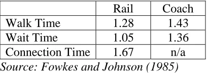
A little reported study focusing on walk and wait time values was conducted as part of the first British value of time study (Fowkes and Johnson, 1985). It involved SP exercises offered to rail and coach commuters. The IVT values of walk time, wait time and, for rail users, interchange connection time are given in Table 2.1. Little variation was apparent according to work arrival time constraints or income. It was concluded that, “The investigation would suggest that the current practice of weighting walk and wait time at twice the in-vehicle figure overstates their importance”. Nonetheless, the study itself (MVA et al., 1987) concluded that the available evidence did not warrant a departure from the convention of weighting walk and wait time as twice in-vehicle time.

Table 2.1: Walk and Wait Time Values for North Kent Commuters

Rail Coach

Walk Time 1.28 1.43

Wait Time 1.05 1.36

Connection Time 1.67 n/a Source: Fowkes and Johnson (1985)

Much subsequent British evidence is covered in the meta-analysis reported in Wardman (2001). This was based on values largely obtained from SP studies and undertaken between 1980 and 1997. It was found that the values of walk and wait time were, on average, valued at 1.66 and 1.47 times IVT.

Wardman and Shires (2001) found walk time at rail stations to be valued at 1.7 times IVT when it involved a change of trains on the same platform but to increase to 2.7 times when it involved crossing to a different platform by means of a bridge or subway. Walk time was valued more highly by females and those with luggage whilst the presence of good or very good facilities for interchanging reduced the value of walk time. The same study valued waiting time at stations, and found it to be higher for females and those on employer’s business trips and to be lower where use could be made of the wait time, where the facilities for waiting were rated as good or very good and for those in the 45-60 and over 60 age groups.

London Transport has commissioned several pieces of research which have addressed how values of walk and wait time vary under different conditions in which they are endured. LT (1985) found the value of ‘unnecessary’ waiting (queuing) to be around three times that of IVT. LT (1977) estimated walking up and down stairs or escalators to be respectively valued at 4 and 2½ times the value of IVT. A more recent study (LUL, 1990) found the weights for walking up and down escalators to be 4.2 and 2.8 and walking up and down fixed staircases to be 4.4 and 3. Similar values were obtained by LT (1985). Higher weights of around 5½ and 4 were obtained for walking up and down emergency stairs (LT, 1995b).

Wardman et al. (2000) covered walking as a main mode as well as time spent accessing a main mode. The latter was valued at 1.9 times IVT in contrast to the 2.7 times IVT when walking time is the main mode. This may reflect non-linearities in the value of walk time with regard to the amount of walk time.

2.3 Other Literature on Walk and Wait Time Values

This section does not aim to provide a comprehensive account of international evidence on the values of walk and wait time but rather a flavour of what has been obtained for comparison with British evidence.

One of the first studies to estimate values of waiting and walking time was Merlin and Barbier (1965). This obtained values of around three times IVT for waiting time and around 1.75 times for walking time. Another early study (Hensher, 1972) estimated the values of wait time and transfer time at twice and 1.5 times IVT respectively.

At a later stage, Bruzelius (1979) observed that walking and waiting time are often valued from two to three times more than IVT. Of the ten disaggregate studies providing walk and wait time values covered in a review of international evidence (TRRL, 1980), walk time was on average valued close to twice IVT and, excepting a study with a very high valuation, wait time was valued around three times IVT.

their adoption is only rarely confirmed by empirical analysis before use”. Table 2.2 reproduces the evidence cited by Bureau of Transport Economics.

Table 2.2: Relationship between Values of In-Vehicle, Walking, Waiting and Transfer Times

Author Source Year Walk Wait Transfer

Merlin & Barbier Quarmby

Hogg Veal

Hoinville & Johnson Hensher Hensher LGORU Ben-Akiva Beesley DOE

Richards & Ben-Akiva Algers, Hansen & Tegner

LGORU

Train & McFadden DTP-DOE BTE France UK Aust UK UK Aust Aust UK USA UK UK USA USA UK USA UK Aust 1965 1967 1970 1971 1971 1971 1972 1973 1973 1974 1974 1975 1975 1975 1976 1978 1.75 2 2 1.7 2 2.9 2.6 2.5 3.5 0.25 0.26 0.47 2 2 2 2 1.5 1.4 2 2 3 3 2 2 2 1.6 3.6 2.5 3 0.25 0.26 0.47 2 2 12 3 3 2 8-11 2 1.5 2 2 1.7 1 1.5 1.5

Source: Bureau of Transport Economics (1982) Table 8.4.

The early evidence as in Britain seems to indicate that waiting time is more highly valued than walk time and that the convention of valuing walk time as twice IVT is more justified than for wait time. Although we have covered some of the material elsewhere, the wait time evidence cited in the review conducted by Waters (1992) also seems to support wait time values in excess of twice IVT.

The more recent national value of time studies conducted in Norway, Sweden, Finland and the Netherlands cast some light on the valuations of walk and wait time.

Subsequent to the main SP experiment conducted in the first Dutch value of time study, a follow-up survey was undertaken relating to public transport users’ values of walk time, interchange time, delays due to schedule failure and a value of wait time based around half the service headway (Gunn and Rohr, 1996). The estimated IVT valuations of these attributes are given in Table 2.3.

Table 2.3: Public Transport Components of Journey Time

Commuting Business Other

Walk time 1.0 1.6 1.3

Interchange Time 2.1 1.6 1.6

Failed Schedule 3.0 1.4 1.4

Half Headway 1.3 1.4 1.7

Source: Gunn and Rohr (1996) Table 5.

Since not all travellers arrive randomly at their boarding point, half the service headway will overstate the amount of waiting time and hence the figures in Table 2.3 will understate the value of wait time. If wait times are a third of headway, and ignoring any convenience benefit of more frequent services, then the value of wait time would be 50% larger than the figures in Table 2.3.

Rather than treating the half-headway term as a value of wait time and for comparison with the headway values reported below, the figures can be halved. Thus the time value of headway is in the range 0.65 to 0.85.

It was concluded that, “Broadly, then, traditional preconceptions (i.e. the experience of previous studies as interpreted by the majority of planners) that components of journey time other than scheduled in-vehicle time are relatively more ‘important’ than in-vehicle time are borne out by this experiment. Traditional weightings, usually a factor of 2 for walking and 3 for wait, seem rather too high”.

Pursula and Kurri (1996) report a model based on bus users’ choices containing time, headway, walking time, transfer walking time and transfer waiting time. Unfortunately, the time valuation relates to total time and hence it is not clear how the values of walk and wait time relate to IVT.

Algers et al. (1996) found the IVT value of transfer time to vary between 1.4 and 2.5, being lower in airports where the transfer is more pleasant than for local bus where it is less pleasant. The time valuation of headway varied between 0.5 for the highest frequency to 0.1 for the lowest frequency. The value of 0.5 seems relatively low, but the highest frequency covered was only two services per hour. The results would suggest that higher values more in line with other studies would be obtained where services are more frequent.

This diminishing effect is consistent with the findings of Algers et al. (1996). The IVT value of headway across ferry, rail and air was 0.37 for leisure journeys less than 50 km but only 0.21 for journeys longer than this. The corresponding figures for business travel were 0.64 and 0.30.

2.4 Public Transport Values of In-Vehicle Time

Many studies in Britain provide estimates of public transport values of IVT whilst one of the strongest effects present in the body of empirical evidence is that there is strong variation in values of time both within public transport and between public transport and car. Two important points must be borne in mind in this context of the value of time and mode.

Firstly, it makes little sense to assess evidence on public transport values independent of the evidence for car users. Secondly, it is essential that we distinguish between two quite separate issues relating to mode. One is that we might expect the value of time to vary across users of different modes, not least because of income variations. We refer to these as User Types. The other is that the value of time may vary according to the mode in which the time is spent, due to differences in the comfort and conditions of travel. We refer to this as Mode Valued. The latter relates solely to IVT although the former relates to all monetary values.

Most of the national value of time studies have estimated public transport values of IVT alongside values for car drivers and we will restrict our attention here to the performance of the various national studies in their treatment of the user type and mode valued issues.

The results for the first British study are reproduced in Table 2.4. The figures are not as informative as they might be due to the estimation in some cases of generic coefficients across modes and the inability of RP models to segment by user type. The values denoted by * and + represent generic coefficients obtained from the same model. The results would seem to indicate that bus users have the lowest values and car users the highest values in the urban context, and the differences are quite substantial. This relationship is consistent with user type effects dominating mode valued effects. However, the pattern is different and less clear for inter-urban travel. The higher value for rail than bus and car for inter-urban leisure would suggest that the user type effect dominates the mode valued effect, whereas the relationship between the bus and car values suggests that mode valued effects are strong. Subsequent analysis (Wardman, 1988) found the bus value for inter-urban commuters to be 17% higher than for train travel.

Table 2.4: First British Value of Time Study: Values by Mode (Mid 1985 prices p/min)

Car Bus Rail

Urban Commute 3.6 & 3.7 2.4* 2.4*

Urban Leisure 4.5 1.25

Inter Commute 3.6 & 4.0+ 3.6 & 4.0+

Inter Leisure 3.8 4.0 5.9

Source: Table 7.1 MVA et al. (1987)

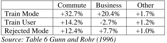
Rohr, 1996). Table 2.5 indicates how values of IVT vary by user type and mode relative to the value of car IVT for car users.

A car driver’s value of IVT on a commuting train journey is therefore 1.492 (1.327 × 1.124) times higher than the value of IVT for a car trip. Train users value car IVT as 1.284 (1.142 × 1.124) times higher than car drivers. Train as a mode is here found to have a higher value than car, with what seem like reasonable variations across journey purpose. It is noticeable that user type has a lesser influence than mode, and whilst this could well be plausibly explained in this context, the inclusion of bus and air users might be expected to lead to more influence from user type.

Table 2.5: Dutch Values of Time Relative to Car Driver Value of Time Amongst Car Drivers

Commute Business Other

Train Mode +32.7% +20.4% +1.7%

Train User +14.2% -2.7% +1.2%

Rejected Mode +12.4% +7.7% +1.0%

Source: Table 6 Gunn and Rohr (1996)

Gunn and Rohr (1996) also report separate SP analysis where, compared to the value of IVT for car drivers in urban traffic, train users had a value of train time which was 6% larger for commuting, 18% lower for business travel and little different for leisure travel. These figures are not entirely consistent with the findings in Table 2.5. For bus and tram users, the values were 9% lower for commuting, 22% lower for business and 25% lower for leisure, indicating the dominance of user type over mode.

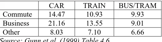
An RP mode choice model specified alternative specific time coefficients for car and train. The train coefficient was 30% lower for commuting trips, 37% lower for business trips and 4% higher for leisure travel. These seem inconsistent with the SP based evidence in Table 2.5, particularly when it is borne in mind that the train time appears to cover the total journey and not just IVT.

Table 2.6: Second Dutch Study: Values of IVT (1997 guilders)

CAR TRAIN BUS/TRAM

Commute 14.47 10.93 9.93

Business 21.16 13.55 9.01

Other 8.03 7.10 6.66

Source: Gunn et al. (1999) Table 4.6.

The Swedish value of time study (Algers et al., 1996) offered car and public transport users SP exercises relating to both their chosen mode and an alternative in order to examine variations in the value of IVT by mode. However, analysis which distinguishes variations in the value of IVT according to user type and mode valued is not reported. The estimated values of IVT, segmented by what seems to be mode valued, are reproduced in Table 2.7. The lower values for car than train and bus, at least for the shorter journeys, are presumably because the effect of mode valued is greater than user type. This might also explain through a fatigue effect the relatively high car value for longer distance trips. However, the distinction between user type and mode valued is not adequately addressed in the above report3.

Table 2.7: Swedish Values of IVT (Swedish Crowns per hour)

Car Air IC

Train

X2000 Reg Train

LD Bus

Reg Bus

Comm <50km 34 54 47 43

Other<50km 27 43 38 28

Trips > 50km 81 88 74 102 70 65 50

Source: Algers et al. (1996)

Ramjerdi et al. (1997) adopted the same approach as the Swedish study in order to examine variations in the value of IVT by mode. Hence each respondent was offered two SP exercises, one relating to their actual mode and the other to an alternative mode. The explicit purpose of this “…. was to evaluate the mode specific differences of the VoT’s”. The data was pooled and separate utility functions estimated by mode. The results reported by mode, which presumably relate to mode valued, are reproduced in Table 2.8. Given that the values are lowest for bus and highest for air, user type is clearly having an influence. However, the report fails to distinguish clearly between user type and mode valued.

3

Table 2.8: Norwegian Values of IVT by Mode (NOK/hr)

Km CAR RAIL BUS AIR Leis EB Leis EB Leis EB Leis EB

<50 38 131 54 124 31 120 151

50-100 101 377 108 104 51 172

100-300 97 207 68 201 53 70 170 258

300+ 77 137 50 105 38 40 151 324

Source: Ramjerdi et al. (1997) Tables 7, 8, 14 and 15.

Pursula and Kurri (1996) conducted separate SP exercises for bus users and car users. The values for bus users relate to total time and were between 10 and 20 FIM/hr depending upon income. The values of time for car users varied between 25 and 50 FIM/hr depending upon road class. As expected, the value of time is higher for car users and the difference is large.

2.5 Current UK Recommendations4

Although individual organisations and companies within the railway industry are free to adopt their own recommendations regarding the value of time, walk time, wait time and headway, the great majority of them use the recommendations set out in the Passenger Demand Forecasting Handbook (ATOC, 1997).

As far as the value of time is concerned, the Handbook adopts the model reported in Wardman (1998a). The latter is a regression based model which explains the money value of time in terms of mode used and mode valued, journey purpose, type of data and distance. It is recommended, although without any empirical support, that the values are amended over time in line with GDP.

The value of walk and wait time involved in access and egressing rail stations is weighted at twice IVT, although time spent accessing the rail network by other modes can have different weights in part influenced by whether there are any money costs involved. An exception to the double weighting of walk and wait time is the connection time at an interchange station. For what appear to be pragmatic reasons relating to application, connection time is given the same weight as train time, although the interchange penalty used not only represents the inconvenience and risks involved in having to interchange but also an element to cover the premium valuation of walk and wait time.

The value of headway used is influenced by the proportion of random arrivals, which is higher for more frequent services, and by a ‘planning penalty’ for those who do not arrive at random. The latter includes an adjustment time element, because rail travellers cannot generally depart precisely when they want to, along with waiting time and the transaction costs of having to find out train times. The time valuation of headway therefore varies across routes and different levels of headway. For all flows, the headway valuation in units of IVT is one for headways of 10

4

minutes or less. At a 30 minute headway it is around 0.8 minutes, falling to around 0.55 and 0.43 for hourly and two-hourly services.

Our understanding is that Transport for London is in the process of reviewing the values of time it uses. The current recommendations are relatively sophisticated, reflecting the unique features of the London Underground in the British context, and are set out in the LT Business Development Manual (LT, 1995a) which specifies weights for different elements of time relative to the value of IVT. Relevant walk and wait time values are set out in Table 2.9.

Table 2.9: LT Weights for Walk and Wait Time

Wait in Uncongested Conditions 2 Wait in Congested Conditions 2 + CF

Acceptable Wait 2

Unacceptable Wait 3

Walk Unimpeded 2

Walk in Congested Conditions 2 + CF Walking Downstairs or Escalators 2.5 Walking Upstairs or Escalators 4

Note: CF represents the congestion factor which is related to the density of travellers on stations.

As far as the value of IVT itself is concerned, these are also set out in LT (1995a). The LUL value is based on the Department of Transport research reported in MVA et al. (1987) with allowance for higher London wages. The LTB value is based on studies relating to bus and is only around a third of the LUL value. At October 1995 prices, the LUL values for working and non-working time were 17.5 and 8.9 pence per minute respectively, whereas the LTB value for non-working time was 3 pence per minute. The latter figure based on DETR recommendations and therefore corresponding to the LUL figures would be 5.5 pence per minute.

2.6 Implications for Our Research

This review of empirical evidence and of recommended values used in evaluation has a number of implications for further research in general and for the direction of this study in particular. These implications are:

• The weights to be attached to walk and wait may well vary across different situations, and in part this may have contributed to the different results apparent across studies. The money values of walk and wait time may vary with journey purpose, user type, journey length and the levels that walk and wait time take. We are not aware of studies which have examined non-linearities in the values of walk and wait time. In addition, the weights to be attached relative to the value of IVT will also vary according to factors which influence the latter numeraire. We will examine variations in the money and IVT valuations of walk and wait time as far as our data will permit.

• Official recommendations do not cover headway yet this is important in evaluating schemes involving public transport options. We will examine British evidence relating to headway values to support the provision of a set of recommended values. The intention is again to examine variations in these values.

• There have been many studies which have yielded public transport values of IVT. However, these cannot be examined in isolation to determine a set of recommended values. It is important that they are compared with car values and the differences between them attributed to the factors that it is possible to incorporate in analysis. This requires analysis of the results of a large amount of empirical evidence. Moreover, for practical application purposes, it may be useful to determine a series of modifiers to obtain public transport values of IVT and values for walk and wait time as a function of car values.

• Although variations in values of IVT by mode are one of the strongest effects apparent in empirical studies, and there have been attempts to distinguish variations in the value of IVT that are due to user type and mode valued, further analysis of these issues, particularly in the British context, is certainly warranted. Meta-analysis provides a means of exploring this issue.

• Current recommendations do not contain variations in values of time by journey length and journey purpose, but this is a less contentious area than the ‘equity’ issues that surround mode. Whilst there is a wealth of evidence that these effects exist, there is no consensus on how they impact on values of time. We would argue that meta-analysis is the most appropriate means of obtaining a consensus view.

3. DATA ASSEMBLY

• Additional data will, in general, lead to more precise coefficient estimates. The variance of the coefficient estimates is inversely related to the number of observations in the model.

• Covering more years will provide more variation in the GDP data and could reduce correlations with other independent variables. The variance of a regression coefficient estimate is inversely related to the amount of variation in the variable to which it relates but is adversely affected by increases in correlation with other variables. In the previous data set, three-quarters of the observations related to the period 1988 to 1994 in which a recession limited the amount of GDP variation.

Table 3.1 lists the number of money values of IVT, walk, wait, access and headway contained within the previous and current data sets. The dominance of valuations of IVT is immediately apparent. Some studies specified an access time term which relates to a combination of walk time and time spent accessing the main mode by means other than walking. As previously, the maximum level of segmentation of values in the data set was mode and journey purpose.

The pre 1980 studies tended to be based on mode choice and to include wait time rather than, as is now more common, a headway variable. This explains the large proportionate increase in wait time values. The data set now contains 719 money values of IVT for analysis purposes, and 1167 values of all the attributes listed in Table 3.1. The 1167 values were obtained from 171 studies. The 38 additional studies covered are listed in Appendix 1.

Table 3.1: Sample of Money Values

Previous Now %Δ

Time 539 719 33%

Walk 131 174 33%

Wait 33 61 85%

Access 46 54 17%

Headway 140 159 14%

Table 3.2 shows the increases in the number of available valuations of walk time, wait time and headway expressed in units of IVT. Not all studies contain IVT and cost coefficients and hence not all contain both IVT and money values of these variables.

Table 3.2: Sample of IVT Values of Walk, Wait, Access and Headway

Previous Now %Δ

Walk 140 183 31%

Wait 34 62 82%

Access 52 60 15%

Headway 145 164 13%

increased data has certainly impacted upon the amount of variation in the measure of income. In the previous data set, the variance of the real GDP per capita measure was 27327. The 31% increase in the data set from 889 to 1167 observations has increased the variance of the GDP measure more than fourfold to 117760.

Table 3.3: Distribution of Money Values

Year Previous Now Year Previous Now

63 3 (0.3%) 87 4 (0.4%) 4 (0.3%)

64 8 (0.7%) 88 21 (2.4%) 21 (1.8%)

67 3 (0.3%) 89 72 (8.1%) 72 (6.2%)

68 3 (0.3%) 90 128 (14.4%) 128 (11.0%)

69 12 (1.0%) 91 80 (9.0%) 80 (6.9%)

70 16 (1.4%) 92 136 (15.3%) 136 (11.7%)

74 3 (0.3%) 93 126 (14.2%) 126 (10.8%)

75 8 (0.7%) 94 108 (12.1%) 108 (9.3%)

80 3 (0.3%) 3 (0.3%) 95 75 (8.4%) 75 (6.4%) 81 4 (0.4%) 19 (1.6%) 96 35 (3.9%) 45 (3.9%) 82 5 (0.6%) 5 (0.4%) 97 26 (2.9%) 37 (3.2%)

83 10 (1.1%) 10 (0.9%) 98 54 (4.6%)

84 5 (0.6%) 9 (0.8%) 99 54 (4.6%)

85 21 (2.4%) 21 (1.8%) 00 74 (6.3%)

86 30 (3.4%) 30 (2.6%)

4. OVERALL VALUES OF TIME

We here present average values of time from our data set, segmented by the key variables of user type, journey purpose and whether the context is one of urban or inter-urban journeys given that the overall average will be strongly influenced by the composition of the sample. The figures provide a general impression of the range of the data and the impact of key variables prior to formal analysis.

The values of IVT are reported in Table 4.1 and are expressed in year 2000 quarter 3 prices. Two sets of figures are given according to the elasticity used to account for differences in real GDP per capita across values. One adjustment uses an elasticity of one as used by DETR in its recommended procedures. The other adjustment involves an income elasticity of 0.5, in line with cross-sectional evidence from the first British value of time study (MVA et al., 1987), the second British value of time study (Hague Consulting Group et al., 1999), studies in the Netherlands (Gunn, 2001) and our previous time series evidence from meta-analysis (Wardman, 2001).

Table 4.1: Overall Values of IVT

Income Elasticity = 1 Income Elasticity = 0.5

Context Mode Mean Std Error Mean Std Error Sample

Car 6.0 0.4 5.5 0.4 64

Bus 4.2 1.0 3.8 0.8 17

Rail 7.2 0.9 6.2 0.7 17

UG 9.2 0.9 8.2 0.8 5

Urban Commute

Car&PT 7.6 0.7 5.8 0.4 44

Car 6.5 0.5 5.8 0.4 73

Bus 2.6 0.3 2.4 0.3 22

Rail 6.5 1.0 5.7 0.8 14

UG 7.3 0.7 6.5 0.6 16

Urban Leisure

Car&PT 4.7 0.5 4.3 0.4 25

Car 13.2 3.6 11.7 3.1 11

Urban Business

Rail&UG 19.2 9.0 17.8 8.3 8

Car 6.4 0.4 5.8 0.4 84

Bus 3.2 0.3 2.9 0.3 27

Urban Other

Other 6.4 0.8 5.5 0.6 29

Car 10.5 1.8 10.0 1.7 11

Rail 12.6 0.8 11.5 0.8 21

Inter Commute

Other 9.1 1.0 7.7 0.9 9

Car 9.2 1.1 8.2 1.0 23

Rail 13.3 1.2 12.0 1.1 44

Car&PT 13.7 1.5 11.8 1.4 10

Air 77.2 19.2 74.2 18.6 4

Inter Leisure

Other 11.7 1.3 10.0 1.1 8

Car 18.3 2.6 17.6 2.6 16

Rail 32.2 3.5 29.3 3.3 34

Rail1st 52.3 5.7 46.0 5.4 17

Car&PT 13.7 1.5 11.8 1.4 11

Inter Business

Air 90.2 19.3 82.4 19.3 12

Car 7.4 0.5 7.4 0.6 10

Rail 17.6 1.5 15.3 1.3 18

Inter Other

Other 8.6 0.9 7.6 0.8 15

DETR recommended values of time (DETR, 2001) for a number of categories are contained in Table 4.2. These are behavioural values and hence directly comparable with those contained in Table 4.1. They have been adjusted from mid 1998 prices and income to 2000 quarter 3 prices and income using the recommended income elasticity of one.

Table 4.2: DETR Values of Time

Business – Driver 39.7 Business – UG 48.1

Business – Rail 57.3 Non Work 8.5

As far as non-work travel is concerned, the DETR recommended values seem to be far too high for urban trips yet too low for inter-urban trips. Across all trips, however, the recommended non-work value compares favourably with the large amount of evidence. The DETR value is clearly an average across different journey lengths, and the findings in section 6 point conclusively to a strong distance effect on the value of IVT. Clearly, the recommended value bears little resemblance to the values by mode, but this is a consequence of using an equity value.

The recommended business values are much higher than the relevant averages in our data set. However, the latter contains valuations obtained for business trips which are based on the employee’s rather than the employer’s willingness to pay. We provide some evidence on the difference between the two in section 6.

Table 4.3 provides summary statistics for the IVT values of walk time in the data set. Unlike the value of IVT, there are few cases for inter-urban travel and hence an overall value is given. For urban travel, the values appear to be less than the convention of twice the IVT value, but otherwise, there seems to be little pattern in the average values. The inter-urban values on average fall well short of two, indicating that walk time is relatively less important on longer journeys. However, we must recall the evidence in section 2 that RP values are higher than the SP dominated values in Table 4.3. This is borne out in the results presented in section 6.

Table 4.3: Overall IVT Values of Walk

Context Mode Mean Std Error Sample

All All 1.68 0.05 183

Car 1.37 0.12 29

Bus 1.67 0.14 10

Urban Commuting

Other 1.99 0.16 29

Car 1.74 0.15 25

Bus 1.66 0.23 13

Urban Leisure

Other 1.97 0.35 9

Car 1.55 0.10 34

Bus 2.02 0.22 13

Urban Other

Other 1.37 0.17 8

Table 4.4 lists the average values of wait time in the sample. Again there are too few inter-urban values to support meaningful segmentation by mode and purpose and it does not make sense to segment the urban values by journey purpose. Underground users appear to have relatively low values of wait time, but overall the value of wait time is little different to the widely used recommendation of twice the value of IVT. However, the results in section 6 indicate that, as expected on the basis of the evidence in section 2, the value of wait time is particularly strongly influenced by whether it is obtained from RP or SP models.

Table 4.4: Overall IVT Values of Wait

Context Mode Mean Std Error Sample

All All 1.76 0.10 62

Bus 1.59 0.22 11

UG 1.17 0.04 11

Urban

Car&PT 2.06 0.14 30

Inter All 1.70 0.28 10

Mean values of headway relative to IVT are given in Table 4.5. The IVT valuations of headway appear to be lower for commuting trips, presumably because these have higher values of IVT. There is little difference between car and bus users. Whilst we might expect car users to be more averse to headway, they may also be more sensitive to IVT changes such that overall there is little difference in the IVT valuation of headway compared to bus users.

Table 4.5: Overall IVT Values of Headway

Context Mode Mean Std Error Sample

All All 0.77 0.04 164

Car 0.85 0.11 18

Bus 0.84 0.20 6

Urban Commuting

Other 0.70 0.17 5

Car 1.00 0.13 19

Bus 0.97 0.17 12

Urban Leisure

Other 0.84 0.12 10

Urban EB All 1.22 0.25 5

Car 0.63 0.07 22

Bus 0.61 0.08 13

Urban Other

Other 0.75 0.03 4

Inter Commuting All 0.47 0.09 7

Inter Leisure All 0.52 0.07 17

Inter EB All 0.69 0.11 14

Inter Other All 0.95 0.17 12

Car 0.63 0.14 7

Rail 0.49 0.08 16

Inter

Those on business value headway relatively highly, although the sample is small. There is also strong evidence that headway is less important for inter-urban trips. In part this could be because the sensitivity to IVT variations increases with distance and in part because travellers are more likely to plan inter-urban journeys and do not expect frequencies to be as high as for urban travel.

These overall figures provide some useful insights into the values of IVT, walk, wait and headway. However, there could be confounding effects at work which such simple disaggregations of the sample fail to detect. A quantitative model which aims to explain variations in individual values of time as a function of relevant socio-economic and trip characteristics would provide a significant advance upon these relatively simple tabulations. It is to such a model that we now turn.

5. META-ANALYSIS: MODELLING APPROACH

In addition to the money and time valuations of the attributes, information has been collected on a range of factors which might explain variations in the valuations. These included the year and quarter of data collection and associated income and retail price indices, sample size, journey distance, type of data upon which the model was estimated, journey purpose, choice context, user type, mode valued, numeraire, location, the omission of non traders and use of logic checks, the means of presenting an SP exercise and the number of attributes in it, the mean level of the attributes and the purpose of the study. It is assumed that the variation in the values which cannot be explained by the above key variables is randomly distributed across the sample.

The variables about which we have collected information are either continuous or categorical. The form of model used to explain variations in the monetary values (V) takes the form:

jk q k jk p j i Z n i i

e

X

V

∏

=

τ

where there are n continuous variables (Xi) and p categorical variables having q categories (Zjk).

We specify q-1 dummy variables for a categorical variable of q levels and their coefficient estimates are interpreted relative to the arbitrarily omitted level. A logarithmic transformation of equation 1 allows the estimation of the parameters by ordinary least squares.

The αi coefficients are interpreted as elasticities, denoting the proportionate effect on the valuation

after a proportionate change in Xi. The exponential of βjk denotes the proportionate effect on the

valuation of a level of a categorical variable relative to its omitted level.

In the models reported in this paper, the dependent variable of equation 1 can take the form of money values of time (section 6) or IVT valuations of walk, wait and headway (section 7).

A simple example of the application of the model based on the units used in this study is given in section 6.1.

6. META-ANALYSIS OF VALUES OF TIME: EMPIRICAL FINDINGS

The analysis reported here is essentially an extension of that previously reported (Wardman, 2001) to incorporate a larger data set, although given the emphasis on IVT, walk time, wait time and headway, we have removed the other valuations relating to departure time changes, search time, late time and time spent in congested conditions. With the exception of departure time changes, the number of observations for these latter values is small. In any event, no additional data was collected for the values of these attributes.

Section 6.1 considers the models estimated to the money values. We then use these models to calculate values of time for a range of scenarios and these are presented in section 6.2

6.1 The Models

Table 6.1 presents models estimated to the data set of IVT, walk, wait and headway valuations and to just the IVT values. The former model contains 1167 observations and the latter 719 observations.

A preferred form of model from many that were tested was identified for the data set relating to all the values. For comparison purposes, the walk, wait and headway values were removed and an otherwise identical model was estimated to the values of IVT alone.

The model is estimated to money values in units of pence per minute and expressed in quarter 4 1994 prices.

Two broad types of variable were examined which we term main effects and interaction effects. Main effects relate to the independent effect of a particular variable, such as distance or mode, on the value of time. Interaction effects are essentially the product of two main effects, thereby permitting, say, the effect of distance to depend upon the mode in question.

The main effects examined in this study were:

• The attribute to which the value relates, which is IVT, walk time, wait time, access time or headway

• Gross domestic product (GDP) per capita in real terms

• Distance in miles, with a further distinction as to whether the journey was over 30 miles and hence classified as inter-urban

• User type which covers car, bus, train, underground and air along with values estimated to various combinations of these users

• The mode to which the value relates, which covers the same categories as user type

• The cost numeraire of parking cost, toll or road user charge, petrol cost, public transport fare or combinations of them

• Whether the value was obtained from Revealed Preference (RP) or Stated Preference (SP) data and whether the SP exercise took the form of a ranking or choice exercise

• Location, which distinguished between London, the South East, metropolitan areas, other conurbations, market towns and rural

• Whether the main purpose of the study was value of time estimation, a valuation study in general or demand forecasting

• Whether public transport cost was presented in single or round trip units

• The choice context of route choice, mode choice or abstract choice

• The means of presenting an SP exercise, which covered the pen and paper method, computer presentation and the use of cards5

• The number of variables in the SP exercise

• The mean level of walk time, wait time and headway in the study in question

• Whether respondents were removed from the data set on the grounds of rationality tests or the absence of trading.

The interactions which we have examined were:

• User type with mode valued, journey purpose, attribute, journey distance, GDP and location

• Mode valued with journey purpose and distance

• Journey purpose with attribute, distance and GDP

• GDP with attribute and distance

• Attribute with distance, means of presenting the exercise and number of variables in an SP exercise

Table 6.1 contains effects that are correct sign and plausible in magnitude, and are either statistically significant or else not significant at the usual 5% level but are considered to merit retention and have t statistics which are not unreasonably small.

Variables removed as not having a significant effect were all the interactions listed above except interactions between user type and mode valued, distance and attribute, user type and attribute, type of data and attribute and limited interactions between purpose and attribute and mode and purpose. It can be seen, therefore, that most interactions relate to differences in valuations across IVT, walk, wait and headway. Main effects that were not significant were numeraires relating to petrol cost, parking charge and public transport fare, locations other than the South East, the main purpose of the study, the choice context, the type of SP exercise, the means of presenting the SP exercise other than the pen and paper method, the number of variables in the SP exercise,

5

the mean level of headway and whether the value was estimated to data sets where respondents had been removed on the grounds of rationality tests or non-trading.

In order to be able to use the model to calculate values, the GDP per capita index has to be known. In 2000 quarter 3, the period for which we subsequently calculate values, this is 3451. In addition, converting from the 1994 period 4 prices in which the model is calibrated to the 2000 period 3 values that we report below requires the values to be multiplied by 1.174 to allow for inflation.

The money value of IVT (VoT) in 2000 quarter 3 prices and income for a commuting journey of 25 miles by train in the South East is calculated as:

min / 43 . 10 ) 25 3451

( 174 .

1 e 5.179 0.634 0.100 0.147 0.723 0.184 p

VoT = − + + + =

where:

• 1.174 is the adjustment to 2000 quarter 3 prices from the 1994 quarter 4 prices of the estimated model

• -5.179 represents the scale factor (constant term in the estimated model)

• 0.634 denotes the rail effect

• 0.147 relates to journeys in the South East

• 3451 is the 2000 quarter 3 GDP index and 0.723 is the GDP elasticity

• 0.184 is the distance elasticity for rail applied here to a 25 mile journey

Other effects apparent in the model and reported below in Table 6.1 do not represent genuine influences on the value of time.

The goodness of fit achieved seem quite respectable, and a large number of statistically significant, correct sign and plausible variations in the values of time have been estimated. The model based solely on the value of IVT achieves a somewhat better fit and, despite the somewhat smaller data set, the precision with which its coefficients are estimated compares favourably with those obtained in the larger data set. This is presumably because values of time tend to be estimated more precisely than values of other attributes.

Table 6.1: Valuation Regression Models

IVT, Headway, Walk, Wait IVT

Variable Coeff (t) Elasticity or Effect Coeff (t) Elasticity or Effect

Intercept -5.179 (4.2) -5.944 (4.6)

Attribute Specific

Head -0.237 (1.7) n/a n/a

Inter Urban

Inter 0.258 (3.5) +29% 0.282 (3.7) +33% Distance Miles +Miles-Head +Miles-WalkWait +Miles-Car 0.184 (6.3) -0.197 (4.1) -0.073 (3.1) 0.075 (3.6) 0.184 -0.197 -0.073 0.075 0.168 (5.4) n/a n/a 0.043 (1.9) 0.168 n/a n/a 0.043 User Type-Mode Valued (IVT)

Car-CarRail Car-Bus Car-CarPT Rail-Rail UG-UG All-CarPT Air-RailAir RailAir-RailAir 0.379 (4.8) 0.714 (4.0) 0.447 (5.7) 0.634 (7.8) 0.482 (3.5) 0.517 (6.9) 1.680 (8.0) 1.403 (5.6) +46% +104% +56% +89% +62% +68% +437% +307% 0.439 (5.7) 0.594 (4.2) 0.449 (6.2) 0.695 (8.9) 0.622 (4.5) 0.554 (7.9) 1.782 (9.0) 1.461 (6.3) +55% +81% +57% +100% +86% +74% +494% +331%

User Type (NON IVT)

Car-Wait Car-Walk Car-Head Rail-Walk RailUG-Wait RailUG-Head PT-WalkWait CarPT-Walk CarPT-Head All-Walk All-Head 0.789 (2.5) 0.694 (3.9) 0.464 (4.1) 0.368 (1.5) 0.612 (3.0) 0.755 (5.2) 0.199 (1.5) 0.232 (2.4) 1.378 (6.6) 0.317 (1.8) 0.879 (4.4) +120% +100% +59% +44% +84% +113% +22% +26% +297% +37% +141% n/a n/a n/a n/a n/a n/a n/a n/a n/a n/a n/a n/a n/a n/a n/a n/a n/a n/a n/a n/a n/a n/a Purpose EB +EB1st +EBFore Comm 0.498 (5.6) 0.754 (5.2) 0.470 (4.3) 0.100 (2.7) +65% +113% +60% +11% 0.559 (6.8) 0.643 (4.7) 0.411 (3.9) 0.164 (3.7) +75% +90% +51% +18% Income

GDP 0.723 (4.6) 0.723 0.823 (5.0) 0.823

Purpose Specific

EB-Head 0.211 (1.5) +23% n/a n/a

Mode and Purpose

Comm-UG 0.520 (2.8) +68% 0.238 (1.9) +27%

Data RP-Walk RP-Wait 0.379 (2.4) 0.886 (5.2) +46% 143% n/a n/a n/a n/a Numeraire

Toll -0.212 (2.2) -19% -0.148 (1.6) -14%

Units

Round -0.076 (1.8) -7% -0.130 (2.6) -12%

Level WalkTime Wait Time 0.271 (8.2) 0.157 (2.4) 0.271 0.157 n/a n/a n/a n/a Region

LSE 0.147 (3.6) +16% 0.068 (1.5) +7%

Presentation

PaperIVT -0.141 (3.1) -13% -0.160 (3.7) -15%

Attribute Specific Variables

Dummy variables were specified for walk time, wait time, access time and headway to determine whether, after accounting for the influences of the other variables in the model, there is any remaining difference in the values of these attributes in relation to each other and to IVT.

The coefficients relating to walk time, wait time and access time were far from statistically significant. We have retained a term for headway (Head) whose effect is not far from significant at the usual 5% level.

Distance Effects

Variations in the value of time are due to variations in the marginal utility of time or money, and there are a number of possible distance related influences on the value of time.

The disutility of a unit of travel time may increase with journey duration, as fatigue, boredom and discomfort set in. Time savings on longer distance journeys will therefore be more highly valued. There may also be a relationship between the values and levels of walk time, wait time and headway. For example, the disutility effect could well operate in the context of progressively longer amounts of walk time. However, this is not specific to the distance of the overall journey and we shall return to this issue below.

The opportunity cost of time spent travelling is presumably greater for longer distance journeys. The activities being pursued must have relatively high utility or importance otherwise their pursuit would not warrant the time and expense of long distance journeys. In addition, there are more pressures on the total time budget where longer amounts of time are spent travelling.

Shorter distance trips tend to be made more frequently. To the extent to which the SP exercise is taken to apply to all trips of the type in question, then a given payment for a time saving implies a larger income effect for more frequent trips. The larger income effect may mean traveller’s are more sensitive to cost variations whereupon shorter distance journeys might have lower values.

Travellers may value variations in cost or time in line with the proportion that they form of total cost or time. However, the effect on the value of time is indeterminate. If the proportionality effect is stronger upon cost (time) then the value of time will increase (fall) with distance, but theory provides no clear indication here. In empirical studies, a logarithmic formulation of the terms in the utility function would be consistent with the proportionality concept6, and this has met with a degree of success (Gunn, 2001). However, whilst it has the potentially desirable property of allowing the value of time to increase with distance, it also exhibits the undesirable property that, for any individual, larger costs will increase the value of time.

The proportionality argument may also apply to walk and wait time, whereupon variations on longer journeys form a smaller proportion of total journey time and are less highly valued.

6

If the utility function of a choice model contains the variable X in the form αlnX, then the marginal utility of X is

Given that congested travel conditions will form a greater proportion of urban travel time, and that this is relatively highly valued but that studies tend not to distinguish between different types of time, then the value of IVT for shorter distance journeys would be higher.

We might expect headway to be less highly valued for longer distance journeys. In part this might be an issue of expectations, since travellers would not regard low frequencies to be unreasonable on longer distance journeys but may well do so on shorter distance journeys. It may also be because longer distance journeys tend to be more planned and hence the convenience of high frequencies is less important.

There may also be an additional effect that leads to lower values of headway at longer distances. At short distances, frequencies are higher and hence random arrivals will be more common. The headway valuation therefore reflects wait time to a greater extent. At longer distances, frequences are lower and the headway value is dominated by schedule delay. Given that wait time is valued more highly than schedule delay, it is not unreasonable that the value of headway is lower for longer distance journeys. However, this is only proxying for the true effect which relates to the level of headway, and we should point out that a significant effect from the mean level of headway on the value of headway could not be obtained.

There might be factors which are correlated with distance and which are not otherwise explicitly accounted for which we can regard as confounding effects. Those with higher incomes may travel longer distances and hence a positive correlation between the value of time and income will become apparent where, as in this study, there is no segmentation of the values of time by income. Other socio-economic characteristics may vary with distance, such as the gender and age distribution and the precise journey purpose within the leisure and business categories. Insofar as males and more senior employees feature more strongly in longer distance travel, the value of time might be expected to increase with distance. However, without far more detailed analysis we cannot draw firm conclusions as to the likely direction of the effect.

Providing that the pattern of correlation with confounding variables remains constant in future, and that the effects of the latter which are discerned by distance are not additionally entered into the evaluation process by some other means, their inclusion within the distance effect does not cause any particular problems. Similarly, the omission from meta-analysis of variables which have only a random effect on the valuations obtained in the different studies is not a cause for concern. However, there may be confounding effects which are a more serious problem because they will influence our conclusions in a misleading way. An example in this context of distance is given by Gunn (2001, p185)

For example, suppose ‘distance’ is an explanatory factor in a meta-analysis of many studies. Suppose some studies are of short-distance choices, some of long-distance. If all the studies examined which had long-distance contexts used large time variations and all the studies examined which had short-distance contexts used small time variations, then a meta-analysis could associate an effect which was truly related to size-of-time-saving wrongly to distance.

One of the strongest and most consistent findings in empirical studies related to the value of time is that the value of IVT is higher for longer trip duration or distance (Thomas and Thompson, 1970; Heggie, 1976; Algers et al., 1996; Hague Consulting Group and Accent, 1999; Gunn, 2001), although admittedly the evidence is not always clearcut (MVA et al., 1987) and indeed sometimes conflicts with the mass of evidence (Ramjerdi et al., 1997).

Most studies simply estimate different models for urban and inter-urban trips or for different time bands, and hence little evidence on the source of the variation is obtained. Some studies allow departures from the conventional linear-additive utility functions. In the context of mode and destination choice, Gunn (2001) reports the log-cost formulation to perform better, implying the value of time to increase with journey duration, although a similar formulation of the time term is not reported. Four reasons were advanced why the log-cost specification performed better. Gunn (2001, p169) concluded that, “All four potential ‘explanations’ of the non-linearity concern distance-based imperfections in the relationship between measured data, behavioural model and actual behaviour, either in terms of information uncertainty to the traveller, or to the modeller”. Appropriate allowance for these effects would reduce the apparent distance effect but not necessarily remove it. However, the distance effect is here proxying for other effects and is not a pure variation in the value of time due to journey duration or cost. Ben-Akiva, Daly and Gunn (1987) do introduce a genuine duration based effect by arguing that due to more binding time budgets the utility function with regard to time might be expected to be convex in contrast to the concavity of the cost term.

Not all evidence points to the superiority of the log-cost formulation. In the context of rail and air mode choice, Wardman and Murphy (1999) found the logarithmic formulation to perform best for both cost and time in the business market, although the leisure market supported a logarithmic function of cost and a linear function of time, whilst RP analysis of choices between car and rail in the inter-urban context choice found support for a logarithmic formulation of both the car time and rail time variables but not of the cost variables (Wardman et al., 1997). The analysis conducted in this study, and reported in Working Paper 561, did not support the log-cost formulation.

Table 6.2 summarises the possible causes of variation in the values of time with distance, the expected impact on the values and the values which it is considered will be affected.

Table 6.2: Summary of Possible Distance Effects

Influence Impact Affects

Disutility Effect Positive IVT

Opportunity Cost/Time Constraint Positive IVT, Walk, Wait, Headway

Income Effects Positive IVT, Walk, Wait, Headway

Proportionate Effect Indeterminate IVT, Walk Wait, Headway

Congestion Effect Negative IVT

Expectations/Planning Negative Headway, Wait

Confounding Effects Indeterminate IVT, Walk, Wait, Headway