Finite Element Method for Analysis of Conjugate Heat Transfer between Solid and Unsteady Viscous Flow

F

INITE

E

LEMENT

M

ETHOD

FOR

A

NALYSIS OF

C

ONJUGATE

H

EAT

T

RANSFER

B

ETWEEN

S

OLID AND

U

NSTEADY

V

ISCOUS

F

LOW

Atipong Malatip, Niphon Wansophark,

and Pramote Dechaumphai

Department of Mechanical Engineering,

Faculty of Engineering, Chulalongkorn University,

Bangkok, Thailand 10330

ABSTRACT

A fractional four-step finite element method for analyzing conjugate heat

transfer between solid and unsteady viscous flow is presented. The

second-order semi-implicit Crank-Nicolson scheme is used for time integration and the

resulting nonlinear equations are linearized without losing the overall time

accuracy. The streamline upwind Petrov-Galerkin method (SUPG) is applied

for the weighted formulation of the Navier-Stokes equations. The method

uses a three-node triangular element with equal-order interpolation functions

for all the variables of the velocity components, the pressure and the

temperature. The main advantage of the method presented is to consistently

couple heat transfer along the fluid-solid interface. Four test cases, which are

the lid-driven cavity flow, natural convection in a square cavity, transient flow

over a heated circular cylinder and forced convection cooling across

rectangular blocks, are selected to evaluate the efficiency of the method

presented.

KEYWORDS

I . Introduction

Conjugate heat transfer between solid and fluid flow, where heat conduction in a solid region is closely coupled with heat convection in an adjacent fluid, is encountered in many practical applications. There are many engineering problems where conjugate heat transfer should be considered, such as in biomedical engineering, design of air-cooled packaging, heat transfer enhancement by finned surfaces, design of thermal insulation, design of solar equipment, heat transfer in a cavity with thermally conducting wall or internal baffle, etc. Most of the research works in this area employ the finite difference method, the finite volume method, the finite element method, and the meshless collocation method as the numerical tools. Convection heat transfer between the solid and the fluid flow is one of the most challenging problems for computational methods due to its inherent coupling between the governing equations of the fluid motion and the energy equation of the solid. This coupling effect can be seen noticeably at high Rayleigh numbers in free convection problems and at high Reynolds numbers in forced convection problems. Another main reason which increases the difficulty in solving the convection heat transfer problems is due to the non-linear phenomenon of the convection terms presented in both the momentum equations and the energy equation. Some algorithms have been proposed and applied to analyze these problems, such as the velocity-pressure segregated method [1-3] based on the SIMPLE algorithm and the unsteady algorithm based on the fractional step method [4-7]. These two algorithms are similar in that they correct the computed velocity components by using the pressure derived from the continuity equation.

Some of the studies in this research area, however, employ the finite difference and the finite volume methods as the numerical tools. He, et al. [8] studied the conjugate problem using an iterative FDM/BEM method for analysis of parallel plate channel with constant outside temperature. Sugavanam, et al. [9] investigated the conjugate heat transfer from a flush heat source on a conductive board in laminar channel flow. Chen and Han [10] showed the solution of a conjugate heat transfer problem using a finite difference SIMPLE-like algorithm. Schäfer and Teschauer [11] used the finite volume method to analyze both the fluid flow behavior and the solid heat transfer together. Aydin [12] studied a conjugate heat transfer phenomenon through a double pane window by using the finite difference technique. Results from these problems showed that both the finite difference and the finite volume methods can perform very well on the problems of interest, but some assumptions on heat transfer coefficients have to be made in order to compute the temperatures along the fluid-solid interface. Furthermore, the unknown temperature and the heat flux at the fluid-solid interface are normally determined in an iterative way, usually through the use of an artificial heat transfer coefficient.

At present, very few computational procedures using the finite element method have been proposed in the literature to analyze such conjugate heat transfer problems. Misra and Sarkar [13] used the standard Galerkin formulation to solve the continuity, momentum and energy equations simultaneously. Malatip, et al. [14] developed a combined SUPG and segregate finite element method for analyzing steady conjugate heat transfer problems. Al-Amiri, et al. [15] used finite element method to study the steady-state natural convection in a fluid-saturated porous cavity of a conducting vertical wall.

The objective of this paper is to develop a second-order time accurate numerical algorithm for analyzing conjugate heat transfer between solid and unsteady viscous thermal flow. The paper extends the splitting finite element algorithm proposed by Choi, et al. [5] to conjugate heat transfer problem [14]. Triangular finite element is employed herein for deriving the associated finite element equations. These triangular finite elements are used together with an adaptive meshing technique to improve the solution accuracy and computational efficiency. The finite element algorithm employs the four-step fractional method with an equal-order triangular finite element. The idea of the consistent SUPG [16, 17] is included in the formulation as an upwind scheme. The time integration method is based on a semi-implicit fractional step method and the resulting nonlinear momentum and energy equations are linearized without losing the overall time accuracy.

ll. Theoretical Formulation and Solution Procedure

2.1 Governing equations

The governing equations for the conjugate heat transfer between the solid and fluid flow are presented briefly in this section. For unsteady incompressible viscous thermal flow where the physical properties of the fluid and solid are independent of the temperature, the governing equations for flow and heat transfer in the solid can be written as follows, Continuity equation,

i i

u x

∂

∂ = 0 (1a)

Momentum equations,

(

)

i

i j j

u

u u t x

∂ ₊ ∂

∂ ∂ = 0

1

(1 ( ))

n n

i i

f i j j

u p

g T T

x x ν x β

ρ

 ∂ 

∂ ∂

− + _ _− − −

∂ ∂ _ ∂ _ (1b)

Energy equation for fluid,

( )

T

u T t x

∂ ₊ ∂

∂ ∂ = f

j j

T Q

x α x

 

∂ ∂ ₊

 

 

∂ _ ∂ _ ɶ (1c)

Energy equation for solid,

T t

∂

∂ = s

j j

T Q

x α x

 

∂ ∂

+

 

 

∂ _ ∂ _ ɶ (1d)

The governing differential equations above are to be solved together with the interface conditions. These include the non-slip condition on the solid wall, while the temperature and heat flux along the fluid/solid interface must be continuous,

, int , int

f s

u = u (2a)

T_{f, int} =T_{s, int} (2b)

, int , int

f s

f s

T T

n n

α

α

∂ ∂ (2c)

where n denotes the normal direction of the interface

Nomenclature

g gravitational acceleration

Gr Grashof number, = gβ T (Th - Tc)L3 / ν2

k thermal conductivity Nu local Nusselt number

Nu average Nusselt number Pe Peclet number

p fluid pressure

Pr Prandtl number, = ν /α

Qɶ heat generation per unit volume Ra Rayleigh number, = gβ T (Th - Tc)L3 / αν

t time

T temperature

u x-component of velocity v y-component of velocity x horizontal distance

y vertical distance

Greek symbols

α thermal diffusivity, = k / ρc

sf

α solid-to-fluid thermal diffusivity ratio, = αs / αf

T

β thermal expansion coefficient

K solid-to-fluid thermal conductivity ratio, = ks / kf

ν kinematic viscosity, = µ / ρ

θ dimensionless temperature, = (T - T0) / (Th - T0) ρ density

Subscripts

i, j nodal quantities int interface o cold surfaces

f fluid

2.2 Fractional four-step method

The governing differential equations are integrated in time by using the semi-implicit four-step fractional method previously proposed by Choi, et al. [5, 6]. The pressure gradient terms are first decoupled from those of the convection, diffusion and the external force terms. The second-order semi-implicit time-advancement scheme of Crank-Nicolson is applied for both the convective and the viscous terms of Eqs.(1b-1c). The pressure is then determined from the continuity equation and the velocity components are corrected by the computed pressure, as follows,

Step 1:

1

(

)

2 ˆ ˆ ˆ n n n n i i

i j i j

j i

u u p

u u u u

t x ρ x

 

− ∂ ∂

+ + = −  

∆ ∂ _ ∂ _ 0

1

(1 ( ))

2

ˆ n

n n

i i

i

j j j

u u

g T T

x x x

ν ∂ ∂ ∂  β

+ _ + _+ − −

∂ _∂ ∂ _ (3a)

Step 2:

1 1 2

* _ˆ n

i i

i

u u p

t

ρ

 

− ∂

=  

∆ _ ∂ _ (3b)

Step 3: 1 2 ∆ * n i

i i i

u p

x x t x

ρ

+ _∂

∂ ∂ =

∂ ∂ ∂ (3c)

Step 4: 1 1 1 1 2 * n n i i i

u u p

t

ρ

+ _{−  ∂} + _

= −  

∆ _ ∂ _ (3d)

Step 5:

(

)

n n n n

j j

j

T T

T u T u

t x + + + − ∂ + + = ∆ ∂ 1 1 2 n n n f

j j j

T T

Q

x x x

α ∂ _∂ + +∂ _+

∂ _ ∂ ∂ _ ɶ (3e)

where ∆t is the time increment, uˆ_i and * i

u are the intermediate velocities, and superscript n denotes the time level. The time increment of the semi implicit method is restricted to achieve a desired solution accuracy, not by the numerical stability. Equation (3e) is also used for analyzing conduction heat transfer in solid by setting the velocity components, uj, to be zero.

2.3 Finite element formulations

The three-node triangular element is used in this study due to the simplicity of the element inter-polation functions. The element assumes linear distribution of the velocity components, the pressure, and the temperature as,

(

)

(

)

{ }

u x y =

∑

(

)

(

)

{ }

v x y =

∑

(

)

(

)

{ }

p x y =

∑

(

)

(

)

{ }

T x y =

∑

where i = 1, 2, 3; and Ni are the element interpolation functions.

The basic idea of the solution algorithm presented in this paper is to use the two momentum equations for solving both of the velocity components, use the continuity equation for solving the pressure, and use the energy equations for solving the temperature in solid and fluid regions. The finite element equations corresponding to the momentum, the continuity and the energy equations, are presented in next section.

2.3.1 Streamline Upwind Petrov-Galerkin method

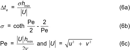
In the streamline upwind Petrov-Galerkin method, a modified weighting function, Wα ,

is applied to the convection terms for suppressing the non-physical spatial oscillation that may occur in the numerical solution. The weighting function is given by [17],

W_α =

h1

1

3

2

h2

h3

where

e

t

∆ = hmin

U

σ

(6a)

σ = coth Pe - 2

2 Pe (6b)

Pe =

2

min

U h

ν and U =

2 2

u + v (6c)

and Pe is the Peclet number, hmin = min(h1, h2, h3) is the minimum element size as

shown in Figure. 1, and U is mean resultant velocity.

2.3.2 Temporal discretization

The method of weighted residuals with the streamline upwind Petrov-Galerkin method is employed to discretize the finite element equations by multiplying Eqs. (3a-e) by weighting functions. Integration by parts is then performed by using the Gauss theorem to yield the element equations as shown in the steps below.

Step 1: Discretization of the momentum equations,

(

)

1 1

2 2

ˆ ˆ

ˆ ˆ

n n

n n

i i i i

i j i j

j j j j

W

u u u u

N d W u u u u d d

t x x x x

α

α α ν

Ω Ω Ω

   

 −  _{Ω +} ∂ _{+ Ω +} ∂ ∂ ₊∂ _Ω

   

 _∆  _{∂  ∂ ∂ ∂ }

     

∫

∫

∫

0

1

(1 ( ))

ˆ

n

n n

i

k i

i j

u p

W d W n d g W T T d

x x

α ν α α β

ρ _{Ω Ω Ω}

 

∂  ∂

= − _∂  Ω + _∂ _ Γ + − − Ω

   

∫

∫

∫

where Ω is the element domain and Γ is the element boundary.

Step 2: The intermediate velocity equations,

1 2

* _ˆ n

i i

i

u u p

N d W d

t x

α α

ρ

Ω Ω

 −  _{Ω =} ∂  _Ω

 _∆  _∂ 

 

 

∫

∫

Step 3: Discretization of the pressure equation,

To derive the discretized pressure equation, the method of weighted residuals is applied to the continuity equation, Eq. (1a),

( )

(

)

1

1 1 ₀

n

n n

i

i i i

i i

W u

W d u d W u n d

x x

α

α α

+

+ +

Ω Ω Γ

∂  ∂

Ω = − Ω + Γ =

 _∂  _∂

 

∫

∫

∫

where ni are the direction cosines of the unit vector normal to element boundary. By

substituting Eq. (3d) into Eq. (9), the following Poisson-type pressure equation is obtained,

Figure 1

(

)

i i i

i i i

W W

t p

d u d W u n d

x x x

α α

α ρ

+

+

Ω Ω Γ

 

∂ ∂

∆ ∂

Ω = Ω − Γ

 

∂ _ ∂ _ ∂

∫

∫

∫

In the above Eq. (11), the unknown uin 1

+

may be approximated by uˆ_i computed earlier as suggested by Kim and Moin [18]. Such approximation gives the error that varies with the time step in the form,

1 _ˆ

n

i i

u + − u

(

)

1 2 n n i p p t x ρ + ∂ − ∆ = − ∂

( )

2 i t p x t ρ ∆ ∂ ∂  ≈ − _{ }

∂ ∂  (11)

Step 4: The velocity correction equations,

1 * n i i u u N d t α + Ω  −  Ω  _∆   

∫

− _{ } Ω

∂

 

∫

Step 5: The temperature correction equations,

(

)

n n n n

j j

j

T T

N d W T u T u d

t x α α + + + Ω Ω  

 −  _Ω+ ∂ _{+ Ω}

   _∆  _{∂ }    

∫

∫

j j j

T T

W d W Q d

x x x

α α

α +

Ω Ω

 _∂ _{∂ ∂} 

 

= _ _ + _ Ω + Ω

∂ _ ∂ ∂ _

 

∫

∫

The finite element equations in matrix from can then be derived by substituting Eq. (4) into Eqs. (7) – (13). The results are as follows:

Step 1:

[ ]

(

[ ] [ ]

)

{ }

2 m ˆi

M

C K u

t   + +    _∆   

[ ]

₍

_{[ ] [ ]}

₎

_{{ }}

_{[ ]}

_{{ } { } { }}

n n n

n

m i gi bi

M

C K u G p R R

t

 

= _ − + _ − + +

∆

  (14a)

Step 2:

[ ]

{ }

[ ]

{ }

[ ]

{ }

2

ˆ_i t _i n

M u + ∆ G p (14b)

Step 3: _K_p_

{ }

{ }

{ }

[ ]

{ }

+

=

[ ]

{ }

[ ]

{ }

2

* n

i i

t

M u − ∆ G p + (14d)

Step5:

[ ]

(

[ ] [ ]

)

{ }

2

n T

M

C K T t +   + +    _∆   

=

[ ]

(

[ ] [ ]

)

{ }

{ }

{ }

{ }

2

n n n

n

T c q Q

M

C K T R R R

t

 

− + + + +

 

 _∆ 

  (14e)

In the above equations, the element matrices written in the integral form are,

[ ]

{ }

Ω

Ω    

∫

[ ]

{ }

j N

W u d

x

Ω

 _∂ 

   Ω

 _∂ _

 

[ ]

  _Ω

 

_∂  _∂

 

 

   

∫

[ ]

j j W N d x x α Ω _∂  _∂ 

  _Ω

  _∂  _∂        

∫

[ ]

{ }

1 i N W d x ρ_Ω

∂  _Ω

_∂ 

 

∫

p K     = j j W N d x x Ω _∂  _∂ 

  _Ω

 

_∂  _∂

 

 

   

∫

{ }

{ }

(

(

)

)

Ω

− + Ω

∫

{ }

{ }

2

i i

W

N u d

t x

ρ

Ω

∂  _Ω

 

   

∆

∫

{ }

{ }

k j u

W n d

x ν Γ ∂  Γ   _∂   

∫

{ }

{ }

(

)

2

ˆ j k

W u n d t

ρ

Γ

− Γ

∆

∫

{ }

{ }

W n d

x α Γ _∂  Γ   _∂   

∫

{ }

{ }

1

s

W q d c

ρ

∫

{ }

{ }

1

W Q d c

ρ

∫

The local time step is assumed as the minimum between the convective local time step and diffusive local time step as,

t

∆ = min

(

)

t

∆ = hmin

U , ∆tdiff =

2 2 min f h α (16b)

2.3.3 Computational procedure

The computational procedure is described in this section and can be summarized as follows:

1. A set of initial nodal velocity components, pressures, and temperatures is given at time n

t =t .

2. Obtain the intermediate velocity components from Eqs. (14a) and (14b). 3. Obtain the pressure, n1

p+ , from Eq. (14c) at time n

t =t + ∆t.

4. Correct the intermediate velocity components, n1

i

u + , from Eq. (14d). 5. Obtain the temperatures,_Tn+1

, from Eq. (14e) at time t =tn+ ∆t.

6. Go to step 1 and repeat the procedure until a desired solution is obtained.

lll. Examples

u(t) = v(t) = 0

u

(t

)

=

v

(t

)

=

0

u

(t

)

=

v

(t

)

=

0

u(t) = 1, v(t) = 0

vortex 1 vortex 2

vortex 4 vortex 3

primary vortex

vortex 5

meshes with triangular elements are employed in the third and fourth to further improve the solution accuracy and computational efficiency.

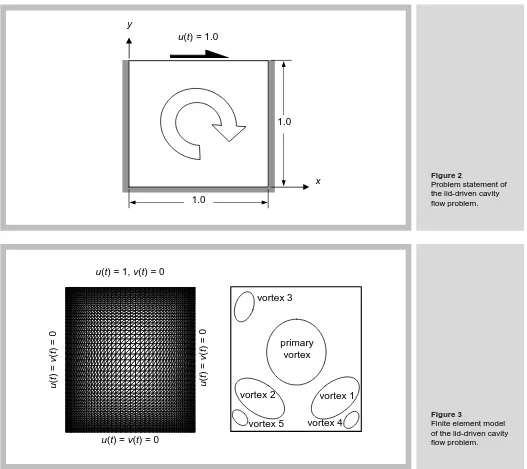
3.1 The lid-driven cavity flow

The lid-driven cavity flow is one of the examples commonly selected for evaluating new numerical algorithms for analyzing viscous incompressible flow. The square cavity has no-slip condition along the bottom and the side walls, while the top-lid moves to the right at the horizontal velocity of one as shown in Figure. 2. The finite element model, consisting of 2,601 nodes and 5,000 elements as shown in Figure. 3, is used in this study.

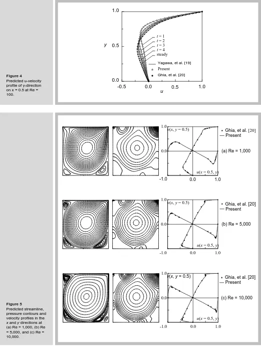
Figure 4 shows the comparative solutions of the u-velocity profiles at the time of 1, 2, 3, and

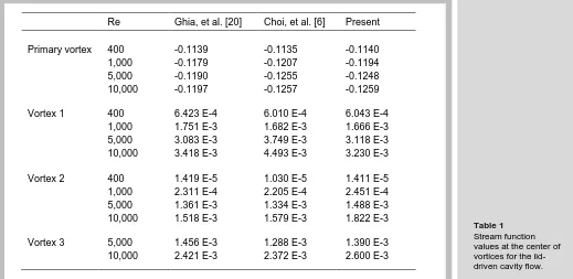
4, all for the Reynolds number of 100. The results are compared with those presented by Yagawa, et al. [19], and the steady-state solution of Ghia, et al. [20]. Figure 5 shows the predicted steady-state solutions as compared to those presented in [20] for the Reynolds numbers of 1,000, 5,000 and 10,000, respectively. These figures show good agreement between the predicted solutions and the solutions obtained from other existing algorithms with time as compared to the results of Malan, et al. [23] and Sampaio, et al. [24]. In addition, table 1 shows the stream function values at the center of primary vortex and the first three vortices as compared to those from Ghia, et al. [20] and Choi, et al. [6].

Figure 2

Problem statement of the lid-driven cavity flow problem. u(t) = 1.0

x y

1.0

1.0

Figure 3

-0.5 0.0 0.5 0.0

1.0 0.5

u y

t = 1 t = 2 t = 3 t = 4

steady

1.0

Ghia, et al. [20]

Present

Yagawa, et al. [19]

Ghia, et al. [20]

Ghia, et al.[20]

(c) Re = 10,000 Ghia, et al. [20] (a) Re = 1,000

u(x = 0.5, y) v(x, y = 0.5)

Present

-1.0

0.0 1.0

0.0 1.0

(b) Re = 5,000 Present

u(x = 0.5, y) v(x, y = 0.5)

-1.0 0.0 1.0

0.0 1.0

Present

u(x = 0.5, y) v(x, y = 0.5)

-1.0 0.0 1.0

0.0 1.0

Figure 4

Predicted u-velocity profile of y-direction on x = 0.5 at Re = 100.

Figure 5

3.2 The natural convection in a square cavity

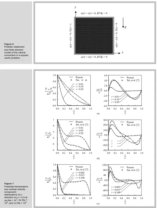
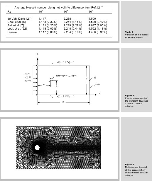
The second example for evaluating the finite element formulation and validating the developed computer program is the problem of free convection in a square enclosure. The square enclosure as shown in Figure. 6, is bounded by the two vertical walls with specified temperatures of one along the left side and zero along the right side, all other boundaries are insulated. The finite element model, consisting of 2,601 nodes and 5,000 elements, is also shown in the figure. Figure. 7(a)-(c) shows the predicted temperature and vertical velocity component distributions at the cavity mid-plane (y = 0.5) that are compared with the results from Sai, et al. [7]. The figures present the comparisons of the transient solutions for the three cases of Ra = 103, 104, and 105. These figures highlight good agreement of the predicted solutions and the solutions from Ref. [7]. Table 2 compares the average Nusselt numbers at the hot wall, Nux=0, obtained from the presented method and the results from the

literatures [6, 7, 21, 22]. The table shows that the solutions from the method presented compare very well with the results from Ref. [21].

3.3 Transient flow over a heated circular cylinder

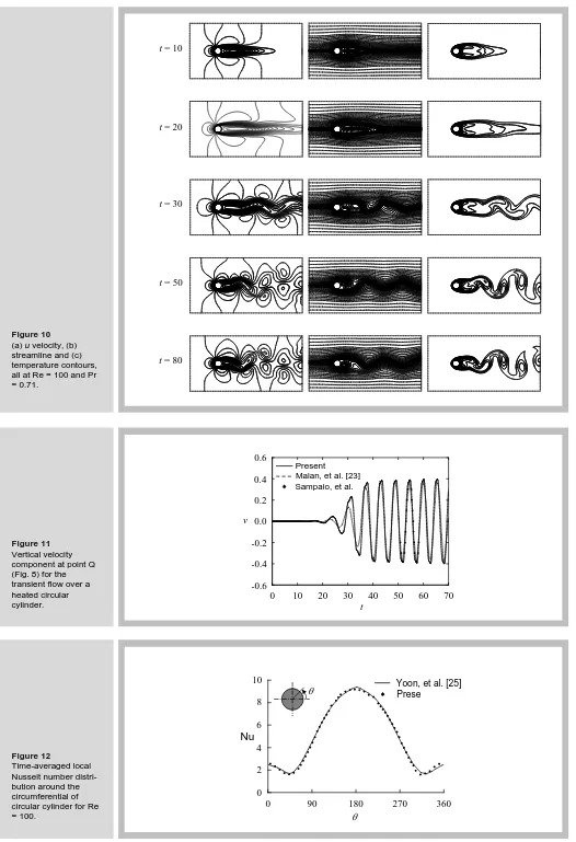
To illustrate the performance of a fractional four-step finite element method for solving transient viscous thermal flow, the problem of a flow past a cylinder is selected as the third example. Such flow past a cylinder is a fundamental fluid mechanics problem of practical importance. The flow field over the cylinder is symmetric at low values of the Reynolds number. However, as the Reynolds number increases, the flow begins to separate behind the cylinder causing vortex shedding which is an unsteady phenomenon. The problem statement and the boundary conditions are shown in Figure. 8. Uniform velocity and temperature profiles are assumed to enter the inflow boundary and the pressure is set to zero at the outflow boundary. The top and bottom boundaries are treated as slip flow with adiabatic condition according to [7, 21, 22] while a non-slip condition is specified on the cylinder surface. A finite element model consisting of 6,485 nodes and 12,734 triangles, as shown in Figure. 9, is used in this study. Figure 10 shows the transient u velocity, streamline and temperature contours at times t = 10, 20, 30, 50, and 80. These solutions are for the case of Reynolds number, Re = 100 and Prandtl number, Pr = 0.71. Figure 11 presents the vertical velocity component at the mid-point of the flow outlet (point Q in Figure. 8) that varies with time as compared to the results of Malan, et al. [23] and Sampaio, et al. [24]. Figure 12 shows the predicted time-averaged local Nusselt number distribution around the circum-ferential of circular cylinder as compared to that given by Yoon, et al. [25]. It should be noted that the average Nusselt number, Nu , was also suggested by Lange, et al. [26] as,

0.5 λ

Nu = 0.082Re + 0.734Re

Re Ghia, et al. [20] Choi, et al. [6] Present

Primary vortex 400 -0.1139 -0.1135 -0.1140 1,000 -0.1179 -0.1207 -0.1194 5,000 -0.1190 -0.1255 -0.1248 10,000 -0.1197 -0.1257 -0.1259

Vortex 1 400 6.423 E-4 6.010 E-4 6.043 E-4 1,000 1.751 E-3 1.682 E-3 1.666 E-3 5,000 3.083 E-3 3.749 E-3 3.118 E-3 10,000 3.418 E-3 4.493 E-3 3.230 E-3

Vortex 2 400 1.419 E-5 1.030 E-5 1.411 E-5 1,000 2.311 E-4 2.205 E-4 2.451 E-4 5,000 1.361 E-3 1.334 E-3 1.488 E-3 10,000 1.518 E-3 1.579 E-3 1.822 E-3

Vortex 3 5,000 1.456 E-3 1.288 E-3 1.390 E-3 10,000 2.421 E-3 2.372 E-3 2.600 E-3

Table 1

where λ = 0.05 + 0.226Re0.085

The present result for the averaged Nusselt number is 5.058, which is 1.36% different from the solution of the equation above.

Figure 6

Problem statement and finite element model of the natural convection in a square cavity problem. u (t ) = v (t ) = 0 , T (t ) = 1

x

y

u(t) = v(t) = 0, ∂T/∂y = 0

u(t) = v(t) = 0, ∂T/∂y = 0

g

Figure 7

Predicted temperature and vertical velocity component distributions of x-direction on y = 0.5 at (a) Ra = 103, (b) Ra = 104, and (c) Ra = 105

(b)

0.0 0.2 0.4 0.6 0.8 1.0 -30.0 -20.0 -10.0 10.0 20.0 30.0 0.0

t = 0.20

t = 0.05

t = 0.01 k L v c ρ L x

0.0 0.2 0.4 0.6 0.8 1.0 0. 0. 0. 0. 0. 1.

t = 0.20 t = 0.05 t = 0.01

T T T ∆ − 0 L x Present Sai, et al. [7] Present

Sai, et al. [7]

(a) 0.0 0.2 0.4 0.6 0.8 1.0 0.0 0.2 0.4 0.6 0.8 1.0

t = 0.20 t = 0.10 t = 0.01

0 T T T − ∆ L x Present Sai, et al. [7]

0.0 0.2 0.4 0.6 0.8 1.0 -6.0 6.0 0.0 4.0 -2.0 2.0

-4.0 _{t = 0.20} t = 0.10

t = 0.01 k L v c ρ L x Present Sai, et al. [7]

(c) 0.0 0.2 0.4 0.6 0.8 1.0 0.0 0.2 0.4 0.6 0.8 1.0

t = 0.100 t = 0.015 t = 0.005

T T T ∆ − 0 L x -40.0 -120.0

0.0 0.2 0.4 0.6 0.8 1.0 -80.0

40. 80.0 120.0

0.0

t = 0.100 t = 0.015 t = 0.005 k L v c ρ L x Present Sai, et al. [7]

Average Nusselt number along hot wall (% difference from Ref. [21])

Ra 103 104 105

de Vahl Davis [21] 1.117 2.238 4.509

Choi, et al. [6] 1.143 (2.33%) 2.264 (1.16%) 4.530 (0.47%) Sai, et al. [7] 1.131 (1.25%) 2.289 (2.28%) 4.687 (3.95%) Leal, et al. [22] 1.118 (0.09%) 2.248 (0.44%) 4.562 (1.18%)

Present 1.117 (0.00%) 2.234 (0.18%) 4.466 (0.95%) Table 2

Variation of the overall Nusselt numbers.

Figure 8

Problem statement of the transient flow over a heated circular cylinder.

u(t)=1 v(t)=0 T(t)=0

u(t) = v(t) = 0, T(t) = 1 v(t) = 0, ∂T/∂y = 0

p = 0 Q

16

8 4

x y

v(t) = 0, ∂T/∂y = 0

4

Figure 9

Figure 10

(a) u velocity, (b) streamline and (c) temperature contours, all at Re = 100 and Pr = 0.71.

t = 20

t = 30 t = 10

t = 80 t = 50

Figure 11

Vertical velocity component at point Q (Fig. 8) for the transient flow over a heated circular cylinder.

-0.6

0 10 20 30 40

-0.4 -0.2 0.0 0.2 0.4 0.6

v

t

50 60 70

Present Malan, et al. [23] Sampaio, et al. [24]

Figure 12

Time-averaged local Nusselt number distri-bution around the circumferential of circular cylinder for Re = 100.

0 90 180 270 360

0 2 4 6 8 10

Nu

θ

θ _Prese

nt

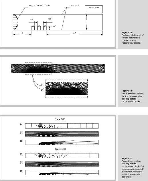
Figure 13

Problem statement of forced convection cooling across rectangular blocks.

Figure 14

Finite element model for forced convection cooling across rectangular blocks.

Figure 15

Forced convection cooling across rectangular blocks (a) pressure contours, (b) streamline contours, and (c) temperature contours.

Q Q Q

0.5 0.5 0.25

u = v = 0 u(y) = 6y(1-y), T = 0

3 9.5

1

Not to scale

Re = 100 (a)

(b)

(c)

Re = 500 (a)

(b)

3.4 Forced convection cooling across rectangular blocks

The problem statement of the fourth example, as shown in Figure. 13, is a flow between parallel plates with three heated fins. The fluid enters with a fully developed profile from the left side and leaves at the right side of the computational domain. The heat generation within the blocks is assumed to be constant and uniform at the value of Qɶ =8. The finite element model, consisting of 5,653 nodes and 10,933 triangles, is shown in Figure 14. Figure 15 shows the predicted pressure, streamline and temperature contours at Reynolds number of 100 and 500, respectively, all at Pr = 0.7, the solid-to-fluid thermal diffusivity ratio,

α

K = 10.

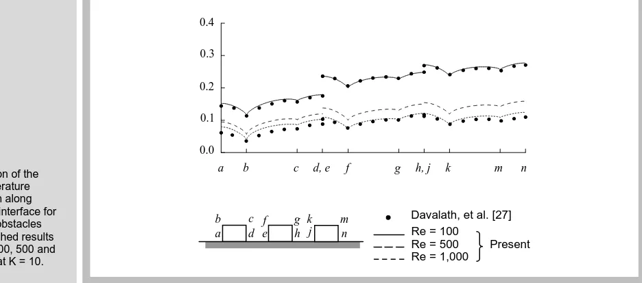
Figure 16 shows the predicted temperature distributions along the fin’s surfaces as compared to the numerical results from Davalath and Bayazitoglu [27] at Re = 100 and 1,000. These figures again highlight good agreement between the predicted solutions and the solutions obtained from the other existing algorithms.

IV. Conclusions

A combined fractional four-step finite element method and streamline upwind Petrov-Galerkin method (SUPG), for analysis of conjugate heat transfer between solid and unsteady viscous thermal flow, was presented. The method combines a viscous thermal flow analysis in the fluid region and a heat transfer analysis in the solid region together. The Navier-Stokes equations are solved by the streamline upwind Petrov-Galerkin method in order to suppress the non-physical spatial oscillation in the numerical solutions. All the finite element equations were derived and presented in detail. The efficiency of the coupled finite element method has been evaluated by several examples that were previously analyzed by using other methods. These examples highlight the benefit of the combined finite element method that can simultaneously model and solve both the fluid and solid regions, as well as to compute the temperatures along the fluid-solid interface directly.

ACKNOWLEDGMENT

The authors are pleased to acknowledge the Thailand Research Fund (TRF) and the 90th Anniversary of Chulalongkorn University Fund (Ratchadaphiseksomphot Endowment Fund) for supporting this research work.

Figure 16

Comparison of the wall temperature distribution along solid-fluid interface for the three obstacles with published results for Re = 100, 500 and 1,000, all at K = 10.

a b c d, e f g h, j k m n

0.0 0.1 0.2 0.3 0.4

Davalath, et al. [27] Re = 100

Re = 500 Re = 1,000

Present

a b c

d

f g j

k m

REFERENCES

[1] J. G. Rice and R. J. Schnipke, "An equal-order velocity-pressure formulation that does not exhibit spurious pressure modes," Computer Methods in Applied Mechanics and Engineering, vol. 58, pp. 135-149, 1986.

[2] H. G. Choi and J. Y. Yoo, "Streamline upwind scheme for the segregated formulation of the Navier-Stokes Equation," Numerical Heat Transfer, Part B: Fundamentals, vol. 25, pp. 145-161, 1994.

[3] N. Wansophark and P. Dechaumphai, "Combined adaptive meshing technique and segregated finite element algorithm for analysis of free and forced convection heat transfer," Finite Elements in Analysis and Design, vol. 40, pp. 645-663, 2004. [4] B. Ramaswamy and T. C. Jue, "Some recent trends and developments in finite element analysis for incompressible

thermal flows," International Journal for Numerical Methods in Engineering, vol. 35, pp. 671-707, 1992.

[5] H. Choi and P. Moin, "Effects of the Computational Time Step on Numerical Solutions of Turbulent Flow," Journal of Computational Physics, vol. 113, pp. 1-4, 1994.

[6] H. G. Choi, H. Choi, and J. Y. Yoo, "A fractional four-step finite element formulation of the unsteady incompressible Navier-Stokes equations using SUPG and linear equal-order element methods," Computer Methods in Applied Mechanics and Engineering, vol. 143, pp. 333-348, 1997.

[7] B. V. K. S. Sai, K. N. Seetharamu, and P. A. A. Narayana, "Solution of transient laminar natural convection in a square cavity by an explicit finite element scheme," Numerical Heat Transfer, Part A: Applications, vol. 25, pp. 593 - 609, 1994. [8] M. He, A. J. Kassab, P. J. Bishop, and A. Minardi, "An iterative FDM/BEM method for the conjugate heat transfer problem

-- parallel plate channel with constant outside temperature," Engineering Analysis with Boundary Elements, vol. 15, pp. 43-50, 1995.

[9] R. Sugavanam, A. Ortega, and C. Y. Choi, "A numerical investigation of conjugate heat transfer from a flush heat source on a conductive board in laminar channel flow," International Journal of Heat and Mass Transfer, vol. 38, pp. 2969-2984, 1995.

[10] X. Chen and P. Han, "A note on the solution of conjugate heat transfer problems using SIMPLE-like algorithms," International Journal of Heat and Fluid Flow, vol. 21, pp. 463-467, 2000.

[11] M. Schäfer and I. Teschauer, "Numerical simulation of coupled fluid-solid problems," Computer Methods in Applied Mechanics and Engineering, vol. 190, pp. 3645-3667, 2001.

[12] O. AydIn, "Conjugate heat transfer analysis of double pane windows," Building and Environment, vol. 41, pp. 109-116, 2006.

[13] D. Misra and A. Sarkar, "Finite element analysis of conjugate natural convection in a square enclosure with a conducting vertical wall," Computer Methods in Applied Mechanics and Engineering, vol. 141, pp. 205-219, 1997.

[14] A. Malatip, N. Wansophark, and P. Dechaumphai, "Combined Streamline Upwind Petrov Galerkin method and segregated finite element algorithm for conjugate heat transfer problems," Journal of Mechanical Science and Technology, vol. 20, pp. 1741-1752, 2006.

[15] A. Al-Amiri, K. Khanafer, and I. Pop, "Steady-state conjugate natural convection in a fluid-saturated porous cavity," International Journal of Heat and Mass Transfer, vol. 51, pp. 4260-4275, 2008.

[16] A. N. Brooks and T. J. R. Hughes, "Streamline upwind/Petrov-Galerkin formulations for convection dominated flows with particular emphasis on the incompressible Navier-Stokes equations," Computer Methods in Applied Mechanics and Engineering, vol. 32, pp. 199-259, 1982.

[17] O. C. Zienkiewicz, R. L. Taylor, and P. Nithiarasu, The Finite Element Method for Fluid Dynamics, 6th ed. Oxford: Elsevier Butterworth-Heinemann, 2005.

[18] J. Kim and P. Moin, "Application of a fractional-step method to incompressible Navier-Stokes equations," Journal of Computational Physics, vol. 59, pp. 308-323, 1985.

[19] G. Yagawa and M. Shirazaki, "Parallel computing for incompressible flow using a Nodal-Based method," Computational Mechanics, vol. 23, pp. 209-217, 1999.

[20] U. Ghia, K. N. Ghia, and C. T. Shin, "High-Re solutions for incompressible flow using the Navier-Stokes equations and a multigrid method," Journal of Computational Physics, vol. 48, pp. 387-411, 1982.

[21] G. De Vahl Davis, "Natural convection of air in a square cavity: A bench mark numerical solution," International Journal for Numerical Methods in Fluids, vol. 3, pp. 249-264, 1983.

[22] M. A. Leal, H. A. Machado, and R. M. Cotta, "Integral transform solutions of transient natural convection in enclosures with variable fluid properties," International Journal of Heat and Mass Transfer, vol. 43, pp. 3977-3990, 2000.

[23] A. G. Malan, R. W. Lewis, and P. Nithiarasu, "An improved unsteady, unstructured, artificial compressibility, finite volume scheme for viscous incompressible flows: Part II. Application," International Journal for Numerical Methods in Engineering, vol. 54, pp. 715-729, 2002.

[24] P. A. B. de Sampaio, P. R. M. Lyra, K. Morgan, and N. P. Weatherill, "Petrov-Galerkin solutions of the incompressible Navier-Stokes equations in primitive variables with adaptive remeshing," Computer Methods in Applied Mechanics and Engineering, vol. 106, pp. 143-178, 1993.

[25] H. S. Yoon, J. B. Lee, and H. H. Chun, "A numerical study on the fluid flow and heat transfer around a circular cylinder near a moving wall," International Journal of Heat and Mass Transfer, vol. 50, pp. 3507-3520, 2007.

[26] C. F. Lange, F. Durst, and M. Breuer, "Momentum and heat transfer from cylinders in laminar crossflow at 10-4 ≤Re≤200," International Journal of Heat and Mass Transfer, vol. 41, pp. 3409-3430, 1998.