with Definitions, Arithmetic and
Finite Domains
Joshua Bax
A thesis submitted for the degree of
Doctor of Philosophy
The Australian National University
November 2017
c
Joshua Bax
First of all, thanks to my supervisor Peter Baumgartner. You were always around to answer my questions and this thesis is in the end, the result of our many discussions. Also I’d like to thank the other members of my panel, Professor John Slaney and Professor Phil Kilby. Thanks also to Uwe Waldmann, for allowing me to share in your research.
Thanks to my office mates and fellow PhD students Jan Kuester and Mohammad Abdulaziz for helping me to understand this business, and for shooting down many stupid ideas late on Friday afternoons. Bruno Wolzenlogel-Paleo was also included in this triage of ideas.
Thanks to Geoff Suttcliffe and Christian Suttner for their efforts on the TPTP library, as well the CASC competition. Without any of those this would have been a brief thesis. Thanks to the CADE conference organizers for monetary support also.
Thanks to Data61 née NICTA, for generous funding, and thanks to the many people there who provided both inspiration and support. I’m proud to have you all as colleagues.
Lastly, thanks to my parents and An Ran for their unwavering support through-out. I really couldn’t have done it without you. Those whom I may have missed, rest assured you have my gratitdue.
This thesis explores several methods which enable a first-order reasoner to conclude satisfiability of a formula modulo an arithmetic theory. The most general method requires restricting certain quantifiers to range over finite sets; such assumptions are common in the software verification setting. In addition, the use of first-order reasoning allows for an implicit representation of those finite sets, which can avoid scalability problems that affect other quantified reasoning methods. These new tech-niques form a useful complement to existing methods that are primarily aimed at proving validity.
The Superposition calculus for hierarchic theory combinations provides a basis for reasoning modulo theories in a first-order setting. The recent account of ‘weak abstraction’ and related improvements make an implementation of the calculus prac-tical. Also, for several logical theories of interest Superposition is an effective decision procedure for the quantifier free fragment.
The first contribution is an implementation of that calculus (Beagle), including an optimized implementation of Cooper’s algorithm for quantifier elimination in the theory of linear integer arithmetic. This includes a novel means of extracting values for quantified variables in satisfiable integer problems. Beagle won an efficiency award at CADE Automated theorem prover System Competition (CASC)-J7, and won the arithmetic non-theorem category at CASC-25. This implementation is the start point for solving the ‘disproving with theories’ problem.
Some hypotheses can be disproved by showing that, together with axioms the hypothesis is unsatisfiable. Often this is relative to other axioms that enrich a base theory by defining new functions. In that case, the disproof is contingent on the satisfiability of the enrichment.
Satisfiability in this context is undecidable. Instead, general characterizations of definition formulas, which do not alter the satisfiability status of the main axioms, are given. These general criteria apply to recursive definitions, definitions over lists, and to arrays. This allows proving some non-theorems which are otherwise intractable, and justifies similar disproofs of non-linear arithmetic formulas.
When the hypothesis is contingently true, disproof requires proving existence of a model. If the Superposition calculus saturates a clause set, then a model exists, but only when the clause set satisfies a completeness criterion. This requires each instance of an uninterpreted, theory-sorted term to have a definition in terms of theory symbols.
The second contribution is a procedure that creates such definitions, given that a subset of quantifiers range over finite sets. Definitions are produced in a counter-example driven way via a sequence of over and under approximations to the clause set. Two descriptions of the method are given: the first uses the component solver
modularly, but has an inefficient counter-example heuristic. The second is more general, correcting many of the inefficiencies of the first, yet it requires tracking clauses through a proof. This latter method is shown to apply also to lists and to problems with unbounded quantifiers.
Acknowledgments vii
Abstract ix
1 Introduction 1
1.1 Thesis Statement . . . 1
1.2 Introduction . . . 1
1.3 Thesis Outline . . . 2
1.3.1 Joint Contributions . . . 3
1.4 An Overview of Automated Reasoning . . . 3
1.4.1 Constraint Solving and SAT . . . 3
1.4.2 Superposition and First-Order theorem proving . . . 5
1.4.3 First-order theorem proving with Theories . . . 7
1.4.4 Satisfiability Modulo Theories . . . 8
1.5 Summary . . . 9
2 Background and Related Work 11 2.1 Motivation . . . 11
2.2 Syntax and Semantics . . . 11
2.3 First-Order Theories for Computation . . . 13
2.3.1 Linear Integer Arithmetic . . . 14
2.3.2 Theories of Data Structures . . . 16
2.3.2.1 ARRAY . . . 16
2.3.2.2 LIST . . . 17
2.3.2.3 Recursive Data Structures . . . 18
2.3.3 Local Theories . . . 19
2.4 Saturation Based Proof Calculi . . . 19
2.5 Superposition for Hierarchic Theories . . . 22
2.5.1 Calculus Rules . . . 24
2.5.2 Abstraction . . . 26
2.5.3 Completeness . . . 28
2.5.4 Definitions and Sufficient Completeness . . . 29
2.6 Other Reasoners with Interpreted Theories . . . 32
2.6.1 SUP(LA) . . . 32
2.6.2 SMT . . . 32
2.6.3 Princess . . . 34
2.6.4 SPASS+T . . . 34
2.6.5 Nitpick . . . 35
3 Beagle – A Hierarchic Superposition Theorem Prover 37 3.1 Motivation . . . 37
3.2 Background Reasoning . . . 38
3.2.1 General Components . . . 39
3.2.2 Minimal Unsatisfiable Cores . . . 43
3.2.3 Other Arithmetic Features . . . 45
3.3 Linear Integer Arithmetic . . . 47
3.3.1 Performance . . . 51
3.3.2 Solution Extraction in Cooper’s Algorithm . . . 54
3.3.2.1 Constructing Solutions . . . 57
3.3.2.2 Performance of Caching in Beagle . . . 59
3.4 Proof Procedure . . . 62
3.4.1 Implementation . . . 63
3.5 Performance . . . 64
3.5.1 TPTP . . . 64
3.5.2 SMT-LIB . . . 67
3.5.3 CADE ATP System Competition (CASC) . . . 68
3.6 Summary . . . 69
3.6.1 Availability . . . 70
4 Definitions for Disproving 71 4.1 Motivation . . . 71
4.1.1 Assumed Definitions . . . 72
4.2 Admissible Definitions . . . 72
4.3 Templates for Admissible Recursive Definitions . . . 75
4.3.1 Admissible Relations . . . 75
4.3.2 Admissible Functions . . . 77
4.3.3 Higher Order LIST Operations . . . 80
4.4 Applications . . . 81
4.4.1 Non-theorems inTLIST . . . 81
4.4.2 Non-theorems inTARRAY . . . 83
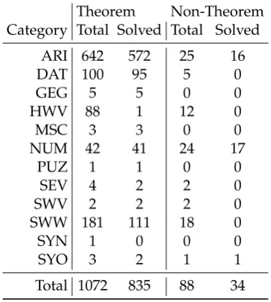
4.4.3 TPTP Arithmetic non-theorems . . . 84
4.4.4 Definitions in SMT-Lib format . . . 85
4.5 Summary . . . 86
4.5.1 Related Work . . . 87
5 Finite Quantification in Hierarchic Theorem Proving 89 5.1 Motivation . . . 89
5.1.1 Overview . . . 90
5.2 Example Application . . . 92
5.3 Finite Cardinality Theories . . . 94
5.3.2 Indexing Finite Sorts . . . 97
5.3.2.1 Finite Predicates . . . 97
5.3.2.2 Finite Sorts . . . 99
5.4 Domain-First Search . . . 100
5.4.1 Clause Set Approximations . . . 102
5.4.2 Update Heuristicnd . . . 105
5.5 Experimental Results . . . 106
5.5.1 Problem Selection . . . 107
5.5.2 Results . . . 108
5.6 Related Work . . . 110
5.6.1 Complete Instantiable Fragments . . . 111
5.7 Summary . . . 112
6 Hierarchic Satisfiability with Definition-First Search 115 6.1 Motivation . . . 115
6.2 Definition-First Search . . . 116
6.2.1 Algorithm . . . 117
6.2.2 Bounded Defining Map . . . 119
6.2.3 Rewiting Clauses with Defining Maps . . . 123
6.3 Updating Defining Maps . . . 125
6.3.1 Clause Labels . . . 127
6.3.2 Finding Update Sets . . . 129
6.4 Experimental Results . . . 131
6.5 Sufficient Completeness of Basic Definitions . . . 133
6.6 Sufficient Completeness of Recursive Data Structure Theories . . . 135
6.6.1 Recursive Data Structure Definitions . . . 137
6.7 Refutation Search . . . 140
6.8 Summary . . . 145
7 Conclusion 147 7.1 Future Work . . . 148
3.1 The Solver interface . . . 39 3.2 Pseudocode for MUC algorithm . . . 44 3.3 Run time in seconds ofBeaglewith and without MUC . . . 44 3.4 Creates the symbolic solution resulting from eliminating all ofxsfrom
F. . . 58 3.5 Run time in seconds ofBeaglewith and without Cooper solution caching 60 5.1 The algorithm for hierarchic satisfiability . . . 101 5.2 denitionalcreates an under-approximation of Nusing global domain∆103 5.3 finddetermines the next exception point to add . . . 106 6.1 Pseudocode for Definition-FirstcheckSATalgorithm . . . 118 6.2 apply rewrites clauseC ∨ ¬∆modulo definitions in MN . . . 123
6.3 clausal transforms defining map M to a clause set without affecting sufficient completeness . . . 124 6.4 Procedure for applying a single update (t≈ α,∆t) to defining map M. 126 6.5 Pseudocode for theNG-MUCheuristic . . . 130 6.6 Thereduceheuristic builds onNG-MUCby subdividing domains . . . . 131 6.7 N is a set of clauses including LIST[Z] . . . 139
3.1 Cooper performance on representative instances of problems . . . 52
3.2 TPTP statistics . . . 65
3.3 Beagleperformance on the TPTP arithmetic problems by category. . . 66
3.4 Beagleperformance on the TPTP arithmetic problems by problem rating. 66 3.5 Performance distribution (count of problems solved in faster time) for different BG solver configurations . . . 66
3.6 CASC-J8 Typed First-order theorem division. . . 67
3.7 CASC-J8 Typed First-order non-theorem division. . . 67
3.8 SMT-lib theorems solved by category. . . 68
3.9 Difficult SMT-lib theorems and their categories. . . 68
4.1 Solving time (s) when conjecture is negated (Ref) and not negated (Sat). 85 5.1 Problems used for testing. Free variables range over the domain ∆ = [0,n−1], where the size parameter n=|∆|is given in Table 5.2. . . 107
5.2 checkSATexperimental results. . . 108
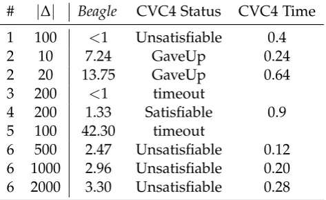
5.3 checkSATcomparison to CVC4. . . 109
6.1 Same problems as in Chapter 5, Table 5.1 but with fixed domain cardi-nality . . . 132
6.2 Run time in seconds of four solver configurations on the problems. . . . 132
6.3 Scaling behaviour (run time in seconds) on problem two. . . 133
Introduction
1
.
1
Thesis Statement
Formalizations of problems in software verification typically involve quantification, equality, and arithmetic. The Satisfiability Modulo Theories (SMT) field has made significant progress in developing efficient solvers for such problems, but solvers for first-order logic have yet to catch up, despite a strong base of equational and quantifier reasoning capability. The reason for this is the high theoretical complex-ity of reasoning with interpreted theories, specifically arithmetic. SMT-solvers also have the valuable capability of providing counter-example models, while first-order solvers are better able to produce proofs of valid theorems.
The Superposition calculus for hierarchic theory combinations provides a sound basis for reasoning modulo theories in a first-order setting. The recent account of ‘weak abstraction’ and related improvements make an implementation of the calculus practical. Also, for several logical theories of interest, Superposition is an effective decision procedure for the quantifier free fragment.
This thesis explores several methods which enable a first-order reasoner to con-clude satisfiability of a formula, modulo an arithmetic theory. The most general method requires that certain quantifiers are restricted to range over finite sets, how-ever, such assumptions are common in the software verification setting. Moreover, the use of first-order reasoning allows for an implicit representation of those finite sets, possibly avoiding scalability problems that affect other quantifier reasoning methods. These new techniques will form a useful complement to existing meth-ods usually aimed at proving validity.
1
.
2
Introduction
The most successful verification technologies today, measured in terms of their use in practical applications to industrial problems, are those of Constraint Programming (CP) and of SMT. These are routinely used for solving difficult optimization and software verification problems.
Using this metric, it appears that the state-of-the-art in first-order theorem prov-ing lags behind. The main technical reason for that is the inherent difficulty in
combining reasoning for quantified first-order formulas with reasoning for special-ized background theories (theorem proving in this general setting is not even semi-decidable). The CP and SMT approaches avoid this issue by dealing with quantifier-free (ground) formulas only, but doing so in a very efficient way.
Not being able to deal with quantified formulas is a serious practical limitation; it limits the range of potential applications, if not the scale. This has been recognized for software verification applications, but currently the limitation is addressed in an ad hoc way: all SMT approaches today rely on heuristic instantiation of quantifiers to deal with quantified formulas. The drawback to heuristic instantiation is that com-pleteness can be guaranteed only in very limited cases. Consequently, such methods will often not find proofs in expected cases, and are not well suited for disproving invalid conjectures stemming from buggy programs. On the other hand, first-order theorem proving approaches inherently support reasoning with quantified formu-las, but lag behind in reasoning with background theories for the reasons mentioned above.
The main hypothesis of this research is that by combining and advancing recent developments in first-order theorem proving, as well as ideas from the CP and SMT fields, it will be possible to design theorem provers that better support reasoning with quantified formulasandbackground theories together.
1
.
3
Thesis Outline
Hierar-chic Superposition allows degenerate models. An advantage of this first method is that it can be implemented with off-the-shelf solvers, at the cost of some inefficiency in computing successive over-approximations. Chapter 6 expands on the method in Chapter 5 by considering the equations that define the over-approximation sep-arately from the clause set. This eliminates some built-in inefficiencies of the prior method and enables an analysis of just which changes are required to advance to the next over-approximation set. The analysis is automatically done with a small prover modification and new heuristics to minimize the resulting change set are given. The abstract description of the method in Chapter 5 can be carried over to create an anal-ogous method that works for recursive data structures and a method for unbounded domains is sketched. The class of basic definitions is defined, which can be excluded from the approximation process yielding further reductions in instantiation. Exper-iments show that heuristics enabled by the more general description do lead to an increase in performance of the definition search.
1.3.1 Joint Contributions
Each chapter except this one and the last are based on papers authored with other people. This section outlines the extent of the reuse of the paper content in each chapter, as well as the new contributions.
Chapter 4 is based on Baumgartner and Bax [BB13]. That chapter provides more general theorems (new) relative to the original results and describes more applica-tions.
Chapter 3 is based on the system description in Baumgartner et al. [BBW15]. Much of the theoretical work in developingBeagleis due to Baumgartner and Wald-mann, and work on the implementation of Beagleis joint work with Baumgartner. The section on solution finding and on LIA examples are original.
Chapter 5 is based on Baumgartner et al. [BBW14]. The original idea underpin-ning this version of the checkSAT algorithm is due to Baumgartner. I contributed an implementation as well as experiments to that paper. The presentation of the al-gorithm in the chapter is new, as are most of the proofs. As said above, Chapter 6 consists of original work.
1
.
4
An Overview of Automated Reasoning
1.4.1 Constraint Solving and SAT
arbitrary relations over arbitrary sets of objects. A concrete definition is given by Dechter [Dec03], as well as an overview of current algorithms and search strategies.
Constraint solving formalizes many common aspects of reasoning problems and this abstract framework allows the development of generic approaches which can be applied to a diverse range of problems. At its core, constraint solving focuses on search strategy and inference. The basic search strategy isbacktrackingand most other methods are essentially refinements of this, for example, lookahead and look-back fall into this category. Inference in constraint solving tries to reduce the search space based on the structure of the problem. The key inference process in con-straint satisfaction is calledconstraint propagation. In this process the constraints are inspected and the domains of variables are restricted in order to enforce varying de-grees ofconsistency; arc-consistency is the weakest– requiring only that an admissible value for a variable is also admissible in every constraint over that variable. Path-consistency is stronger, it requires that any assignment to a pair of variables can be extended to a full solution.
For certain combinations of constraints a higher level of consistency is desired: a common example is when there are many mutual disequations, for example, when assigning drivers to buses, no driver simultaneously drives two buses. Enforcing low-level consistency on the variables participating in these constraints often does not produce any useful inferences, and enforcing high-level consistency on the problem is costly. Instead, a middle ground is struck and consistency is enforced only for the disequation constraints. The regularity of these constraints yields an efficient algorithm for consistency based on matchings on bipartite graphs. Constraint solvers provide a modelling abstraction called anallDifferentconstraint that allows replacing the individual disequations with a single equivalent constraint. The new constraint can be solved using a specialized algorithm. In general many such constructions have been given for problems such as solving weighted sums or bin packing problems, these are known asglobal constraints.
Finite constraint satisfaction problems have been shown to fall in the fragment of effectively propositional (EPR) formulas of first-order logic [Mac92]. Formulas in the EPR fragment are equivalent to (possibly very large) finite sets of ground formulas– hence they can be solved by a SAT/SMT solver. Conversely, SAT is itself a specific instance of a constraint satisfaction problem. The fact that the two approaches can be translated between in no way implies such a translation would be efficient, and there are other respective benefits to the two approaches besides. A good comparison of SAT with CP can be found in Bordeaux et al. [BHZ05].
SAT also focuses on both search and inference, although the language and data structures it uses are much more restricted than that found in CP problems. In CP, problems are modelled directly, often natively in the programming language of the library– most problems treated by SAT solvers are translated via a specialized tool into propositional formulas. Furthermore, SAT is a push-button/black box technol-ogy focused on verification only, while CP is mostly open and programmable and can do optimization as well as verification.
Sometimes the use is explicit: as a theory solver for SMT [Nie10], otherwise the use is implicit, specifically using the underlying algorithms to improve various reasoning tasks [BS09, Mac92]. This was a motivation for the Finite Model finding technique, which is described below.
1.4.2 Superposition and First-Order theorem proving
First-order logic theorem proving aims to develop push-button verification technol-ogy for recognizing first-order logic theorems. First-order logic is expressive enough to encode almost all modern mathematics and, as would be expected, is undecidable. However, classical results also show that the set of valid formulas of first-order logic is in fact enumerable– this follows from the existence of effective calculi whose rules produce valid formulas from a set of axioms. From Herbrand’s theorem and the compactness theorem it follows that any given unsatisfiable formula can be demon-strated as such by finding a finite set of instances of the formula which do not have a model. It is this result that underlies automated theorem proving and defines its limitations: if the given formula is not valid the solver may never be able to prove it so. So first-order theorem provers are at best semi-decision procedures for first-order logic.
First-order proof calculi designed specifically for automation had their origin with Robinson’s Resolution method in the early 60’s [Rob65b], followed by the introduc-tion of the Paramodulaintroduc-tion calculus [RW69], which introduced a dedicated inference rule to deal with identity. Later refinements used orderings to restrict the proof search; methods extending the Knuth-Bendix completion method to first-order logic are known as Superposition calculi [BG98, NR01] and are generally considered to be state-of-the-art when theorem proving over equational theories.
The resolution calculus comprises the following basic rules:
Resolution L ∨ C ¬M ∨ D
(C ∨ D)σ
Factoring L ∨ M ∨ D Dσ
in both casesσ is a most general unifier ofLandM.
Though meeting with some early success, it was soon recognised that resolution had severe shortcomings when using theories involving equality. In particular, reso-lution on the transitivity axiom and reflexivity axioms produce infinitely many new clauses. The Paramodulation calculus was developed to deal more effectively with equality. It adds a new inference rule to the resolution calculus, which encodes the familiar ‘replace like by like’ rule for equality:
Paramodulation C ∨ s≈t D[u]
(D[s] ∨ C)σ
whereσ is the mgu oft andu
However, the Paramodulation calculus fell short of its goal– it was found that the paramodulation rule still produced too many irrelevant clauses to be useful.
An approach that helped to push forward development of first-order theorem proving is Knuth-Bendix completion [KB83]. Essentially, it is a method for trans-forming a set of equations into a new, ordered set of equations which, when applied non-deterministically, constitute a decision procedure for the word problem of the original algebra.
This method was generalised from single ground equations to full first-order clause logic, and the orderings used in the Knuth-Bendix method were found to confer a strong enough restriction on the productivity of the paramodulation rule to make it practically useful. This development is reviewed in Bachmair and Ganzinger [BG98]. The combination of the paramodulation rule along with the ordering strategy of Knuth-Bendix completion is known as Superposition.
Positive-Superposition C ∨ s ≈t D ∨ u[s
0]≈ v
(C ∨ D ∨ u[t]≈v)σ
whereuσ6vσandsσ6tσ,(s ≈t)σ;(u≈v)σare maximal in their respective clauses,(s≈t)σ6(u≈v)σands0 is not a variable.
1.4.3 First-order theorem proving with Theories
It was recognised some time ago, that the efficiency of reasoning could be improved by incorporating knowledge about existing theories into the reasoning process. Ini-tially first-order theorem proving aimed to address the question of satisfiability of the input formulas in full generality, though it is hardly useful when one is extending a particular theory with a fixed interpretation– say that of lists or of linear arithmetic. This approach would add theory axioms to the input and apply the proof procedure to the extended set of formulas. The problem is then, that it allows non-standard interpretations of the theory in question, and it is impossible when the theory is not finitely axiomatizable.
Stickel [Sti85] describes Theory Resolution, which generalizes the resolution cal-culus by allowing a resolution inference on clause literals which are possibly not syntactic complements but are complements modulo the theory in question. For ex-ample, 1 < x and x−1 < 0 do not unify in the standard sense but together are unsatisfiable in the theory of arithmetic. It is also shown that this is a generaliza-tion of the Paramodulageneraliza-tion calculus (theory resolugeneraliza-tion with the theory of uninter-preted functions and equality). However, to admit this generalization one needs the ability to compute all potential theory unifierswithin the given theory– of which there may be infinitely many. For example, unifying p(x+y) and ¬p(11) yields
[x7→1,y 7→10],[x7→2,y 7→9]. . ..
Bürckert [Bür94] gives a thorough treatment of this problem for the resolution calculus. Theory literals are removed from clauses by a process of abstraction and added to a constraint subclause. Effectively, each clauseCis translated to a logically equivalent formulaD→E, whereDis a conjunction of theory literals only, andEis a disjunction of strictly non-theory literals. Resolution is performed on the non-theory part of clauses, and constraints are accumulated until a (not-necessarily unique) con-strained empty clause is derived. The constraint (a conjunction of non-ground theory literals) is checked by an appropriate theory solver, and if the constraint is satisfiable, the satisfying model is removed from consideration. Once all possible models have been eliminated in this way, the proof search terminates. The advantage of this approach is that all theory literals are excluded from the proof search, drastically reducing the search space. A shortcoming is that too much is assumed of the theory solver, in particular, when combining the theory of equality of uninterpreted func-tions with other theories (the theory solver should be able to deal with any user defined functions which range into the other theories). However, this is typically not the case, as the theory of the solver is usually fixed.
A more workable approach is that of Bachmair et al. [BGW94], who use the framework of Hierarchical Specifications to allow a Superposition calculus to con-servatively extend fixed theories. This is the subject of Chapter 2.
1.4.4 Satisfiability Modulo Theories
SMT-solvers combine SAT solving with dedicated theory decision procedures. An introduction to SMT solvers can be found in Barrett et al. [BSST09], while a good summary of the main decision procedures used in SMT solving is in Bradley and Manna [BM07].
The decoupling of solvers is advantageous, as it allows both the SAT solver and the theory solver to be pluggable. So a single SMT implementation can be updated to use the latest SAT technology, as well as support multiple theories within a com-mon reasoning framework. Theory decision procedures must decide satisfiability of conjunctions of ground literals within the language of the theory. Classic decision procedures include those for theories of Equality, Linear Integer Arithmetic, Arrays, Lists and other inductive data types, and fixed-width bitvectors.
Commonly, verification tasks involve several of the above theories in combination. The Nelson-Oppen procedure [NO79] is used to allow decision procedures for sepa-rate theories to coopesepa-rate, together deciding satisfiability for conjunctions of ground literals in the combined theory. This procedure requires that the signatures of the background theories are disjoint, and may not be possible where one of the theories is finite.
The restriction to ground formulas imposed by decision procedures for the indi-vidual theories gives good performance guarantees, but means that quantified for-mulas must be reduced to ground forfor-mulas by other means. In general, forfor-mulas ∀x.F[x]are successively ground instantiated with theory terms until an unsatisfiable set of instances of Fis found. Various methods [GBT07, GdM09, DNS03] have been proposed that identify instances to use for instantiation, or quantified fragments of theory languages which admit instantiation to a set of equi-satisfiable ground in-stances. SMT solvers are normally used as part of larger verification environments such as Isabelle/HOL or ACL2, or as part of specification languages which man-age the translation of verification conditions into complete fragments. Examples of such specification languages are Boogie [BCD+05] and Why3 [FP13], which sup-port full-blown implementations of verification languages (e. g. , Dafny [Lei10] and Frama-C [KKP+15], respectively), and interface with SMT solvers to discharge their verification conditions.
Some work has been done towards using constraint solvers (particularly spe-cialised propagators), as theory solvers with this method as well as applying more general ideas from constraint solving to SMT and SAT. For example, Nieuwen-huis [Nie10] suggests this, as well as using more general CP heuristics in the SAT part of the SMT procedure. Conversely, it has been noted that CS problems are in-stances of SMT problems, and so SMT techniques can be applied in that direction too [NOT06, BPSV12]. First-order theorem provers have also been adapted to work as theory solvers for SMT, in particular, superposition based methods are investi-gated by Armando et al. [ABRS09] as theory solvers for many theories, with criteria for combinations of theories also described.
1
.
5
Summary
Theorem proving over bounded domains with arithmetic is a difficult problem class with applications in bounded model checking, formal mathematics, and other verifi-cation tasks. It can be translated from first-order logic to a constraint satisfaction or SAT problem (for which efficient tools exist), however, a direct translation from one to the other is often inefficient. SMT solvers may also encounter problems when instan-tiating quantifiers in the original problem. A different approach is to take a first-order solver based on the calculus given in Baumgartner and Waldmann [BW13b] and mod-ify it to produce a decision procedure for the restricted case considered. While simple cases have been treated (or fall under existing generalizations which have strong as-sumptions), an important question still remains: how can new functions be added to the theory without losing decidability (for finite domains), or completeness in the general case? This is illustrated in the following simple example.
Example 1.5.1 (Loss of Completeness for Introduced Functions). Let f4 be a new operator symbol that maps integers to integers. It will represent a permutation on {1, 2, 3, 4} ⊂ Z. The assumption that this is a subset of integers will entail that the elements are distinct. The following formulas assert that f4 is a permutation on the appropriate set:
∀x:Z,y:Z.((1≤ x ∧ x≤4 ∧ 1≤y ∧ y≤4)⇒(f4(x)≈ f4(y)⇒x ≈y))
∀x:Z.(1≤ x ∧ x≤4)⇒ ∃y:Z.(1≤y ∧ y≤4)∧ (f4(y)≈x)
The goal will be to show that if 1 and 2 are members of 2-cycles and f4(3) =3 then f4(4) =4, i. e. , f4 is(1, 2)in cycle notation. Formally, the solver must show that the formula
(f4(f4(1))≈1 ∧ f4(f4(2))≈2 ∧ f4(3)≈3) ∧ f4(4)6≈4
Background and Related Work
2
.
1
Motivation
This chapter covers the definitions and lemmas required in each chapter of the the-sis. Section 2.2 gives an account of first-order logic syntax and semantics, specifically monomorphic (sorted) equational logic. Section 2.3 describes some logical theories. The additive theory of integers is used as an interpreted theory in most examples while the data structure theories are used as a source of problems and to provide context for applications. Section 2.4 describes some common notions from saturation based proof calculi, in particular definitions of terms, term algebras and substitu-tions are used throughout. Section 2.5 describes a specific calculus for reasoning in hierarchic combinations of theories. This calculus will form the basis for the imple-mentation in Chapter 3 and will be the reasoning component used in other chapters Section 2.6 describes other reasoners that use either integers or incorporate back-ground reasoning in some way.
2
.
2
Syntax and Semantics
Throughout this thesis, the following standard account of first-order logic with equal-ity will be used.
The logic ismany-sorted: each term is assigned a sort. The type system employed is monomorphic, all of the sorts are constant symbols with no internal structure. Concretely, a many-sorted logic restricts the set of values that can be assigned to variables and restricts both terms in an equation to have the same sort. Sorts are assumed to be non-empty in every interpretation and distinct sorts are disjoint.
A signature Σ is a tuple (Ξ,Ω) consisting of a finite set of sort symbols Ξ =
{S1, . . . ,Sn}and set of operator symbolsΩwith associatedaritiesover the sorts inΞ, written f :S1×. . .×Sn→S for example.
All signatures are a assumed to have at least the Boolean sort Bool, as well as the constant symbol true. Predicate applications, e. g. , p(x), are modelled by the atomic equationp(x)≈true(where≈is the logical symbol for equality) and negated predicate atoms ¬p(x) by p(x) 6≈ true. These are usually abbreviated to the non-equational form in the text. Only predicates andtrue have the sortBool, in particular
there are noBool-sorted variables.
A signatureΣis asub-signatureof another signatureΣ0, writtenΣ⊂Σ0, if all sorts
and function symbols ofΣare included inΣ0, with the arities of the function symbols unchanged. Then Σ0 is referred to as anextensionof Σ. In most cases, the extension signature adds function symbols only, e. g. , in Skolemization, and when the new function symbol needs to be identified the extension signature will be written Σ ∪ {f}, for example, abbreviating(ΞΣ,ΩΣ ∪ {f}).
Given a signature Σ, and a countable infinite set of variable symbols X, such that for each S ∈ Ξ,X contains infinitely many variables of that sort (exceptBoolof course), then the set ofΣ-termsT(Σ,X)is defined inductively as:
1. Any x∈ X or 0-aryconstantsymbolc∈ Σ
2. f(t1, . . . ,tn)for all f : S1×. . .×Sn → S ∈ Ω and allΣ-termst1, . . . ,tn having sortsS1, . . . ,Snrespectively.
Terms inT(Σ,∅)are calledground terms.
Arbitrary variables appearing in the text will be written using x,y,z; constants written a,b,c,d; and applications of function symbols f,g,h to terms: f(s,t),g(x), for example. Terms in general are represented with lettersl, . . . ,t. Boolean terms are called atomic formulas, oratomsfor short.
Logical symbols include the usual Boolean connectives ∧,∨,¬,⇒; quantifiers ∀,∃; and equality, denoted by≈. Equality (≈) is not included in the signature as it is a logical symbol. As such, it is always interpreted as an equivalence relation, so the equality axioms (reflexivity, transitivity, symmetry and functional congruence) are superfluous. The symbol= denotes identity of mathematical objects in meta-logical statements.
That a term t has sort S, is indicated by t : S in variable lists of quantifiers or in running text. To indicate the sort of a subterm in a formula or of both terms in an equation, a subscript is used, e. g. , ina ≈S bbothaandbhave sortS.
Since sorts are assigned disjoint sets, terms in an equation must be of the same sort; it is assumed that all well-formed formulas satisfy this requirement (well-sortedness). The language of Σ is the set of all well-formed formulas made from Σ-terms.
AninterpretationI of a signatureΣconsists of
• adomainDI ={ξ1, . . . ,ξn}that interprets the sortsΞ={S1, . . . ,Sn}ofΣ, and • anassignmentwhich maps from function (and constant) symbols f : S1×. . .×
Sn →Sk ofΩton-ary functions fI :ξ1×. . .×ξn→ξk.
It is required that the sorts are inhabited, i. e. , no ξi is empty and that they are pairwise disjoint.
An interpretation defines a unique map from terms in T(Σ,∅)to DI, the image
ground equations is defined according to the usual truth tables. A valuation ν for interpretation I is a map from X to DI. Valuations lift homomorphically to terms,
atoms, and formulas; simply replacing variables consistently in their contexts. Then, an existential formula ∃x1, . . . ,xk. F is satisfied if there is an interpretation I and valuationνoverI such thatI satisfiesν(F). It is assumed that universals abbreviate negated existentials. (Note that Section 2.4 gives a slightly different semantics for clauses).
Given Σ0 and sub-signature Σ, the Σ-reduct of a Σ0-interpretation is the unique Σ-interpretation obtained by restricting the domain to just the sorts of Σ. Since the function arities ofΣdo not include sorts fromΣ0, the interpretation of these symbols does not change in theΣ-reduct.
A logical theory is simply a set of interpretations of the same signature, closed under isomorphism. The theory axiomatized by a set of Σ-formulas (the axioms) is the maximal set of Σ-interpretations that satisfy those axioms, again, closed under isomorphism. Then, given a theory Twith signatureΣ, a Σ-formula isT-satisfiable if someI ∈T satisfies it, andT-validif allI ∈T satisfy it.
The entailment symbol ‘|=’ is used in several ways in this thesis. Assumeφ is a Σ-formula or clause, Tis a theory with signatureΣ,I is aΣ-interpretation, andN is a set ofΣ-formulas (or clauses), then |=can be used
• As shorthand for ‘satisfies’. IfI satisfiesφ, thenI |=φ.
• To indicate logical entailment between formulas.N |=φiff every interpretation that satisfies all formulas ofN also satisfiesφ.
• To indicate entailment by a theory. T |=φiff everyI ∈T satisfiesφ.
• To indicate logical entailmentrelativeto a theory. N |=T φiff every I ∈ T that satisfiesN also satisfies φ.
The statements T |=⊥, andT |= (empty clause) are shorthand for Tbeing unsat-isfiable.
The quantifier-free fragmentof a language is the subset of the language built with-out quantifiers, where unbound variables are treated as if they were existentially quantified. The quantifier-free conjunctive fragment is a sub-fragment of the above which only contains conjunctions of possibly negated atoms. Some authors do not make this distinction, since any decision procedure for satisfiability of formulas in the quantifier-free conjunctive fragment can be made into a decision procedure for satisfiability in the quantifier-free fragment by transforming a given formula to dis-junctive normal form and testing each disjunct in turn.
2
.
3
First-Order Theories for Computation
decidability results of Nelson and Oppen [NO80] have influenced the choice of ax-iomatizations of recursive data structures.
2.3.1 Linear Integer Arithmetic
Presburger Arithmeticis the language of arithmetic over the natural numbersN with-out multiplication. Though lacking in expressivity, Presburger formulas arise fre-quently in software verification: simple while-loops can be modelled [BMS06], and both integer valued linear programming problems and constraint satisfaction prob-lems, can be expressed with Presburger Arithmetic formulas. Furthermore, the the-ory allowsquantifier elimination: each quantified formula is equivalent to a quantifier-free (ground) formula, and so the first-order theory is decidable.
The decidability of Presburger Arithmetic was shown by M. Presburger [PJ91], and the quantifier elimination procedure used today was given by Cooper [Coo72]. The latter procedure works in a language extended with multiplication and division by constant coefficients, whose theory is equivalent to Presburger Arithmetic.
The signature of Presburger Arithmetic isΣP= {0,s1,+2}, where 0 is a constant, s1is the 1-ary successor function and+2is addition, written infix. The only sort apart from Boolis SN, the sort of natural numbers. The axioms for Presburger arithmetic are:
(1) s(x)6≈0 (2) s(x)≈ s(y)⇒x≈y
(3) x+0≈x (4) x+s(y)≈s(x+y) (5) (φ[0] ∧ ∀n.(φ[n]⇒φ[n+1]))⇒ ∀x.φ[x],
whereφis anyΣP-formula with one free variable.
The language of Presburger Arithmetic is too cumbersome for most applications in software verification. More common is Linear Integer Arithmetic (LIA) which has signature ΣZ = {. . . ,−2,−1, 0, 1, 2, . . . ,−1,+2,<2}; the sort of integers S
Z is the only sort. The axioms of LIA are those of a linearly ordered Abelian group where {0,−,+,<} have their expected roles. Its canonical model is Z with the natural addition function and order relation. The theory of LIA is equivalent to Presburger arithmetic asΣZ-formulas can be directly translated toΣP-formulas [BM07].
Cooper’s Algorithm: Cooper’s algorithm [Coo72] for quantifier elimination in LIA (and therefore, for deciding TZ-validity of ΣZ-formulas) is well known. Although formulas with arbitrary quantifier structure can be checked, the complexity of the procedure is very high: Oppen [Opp78] gives an upper bound time-complexity of 22cn for formulas of lengthnand some positive constantc, while Fischer and Rabin [FR74] show that for most lengthsnthere is some formula which will take at least 22dn steps to check validity, for some constant d. Despite this, Cooper’s algorithm has the advantage of being well understood, e. g. , optimizations are already described in Reddy and Loveland [RL78], and implementations including various optimizations are described elsewhere [Har09, PH15, BM07]. Moreover, it is advantageous to have a single algorithm that can discharge proof goals of varying complexity. Consider the use of Cooper’s algorithm in the Isabelle/HOL proof environment1: the well-known proofs of correctness allow for a verified implementation and the algorithm’s generality allows it to be used as a component solver in the proof assistant.
The relationship between complexity and quantifier structure for Peano Arith-metic formulas has also been investigated. Reddy and Loveland [RL78] show that for formulas of lengthnwithm>0 quantifier alternations, complexity is just 22cnm+4 for constant c > 0. More specifically, Haase [Haa14] shows that Presburger Arith-metic formulas with fixed quantifier alternations arecompletefor respective levels of the weak EXP hierarchy. Woods [Woo15] shows that sets described by Presburger formulas are exactly those sets which have rational generating functions.
Cooper’s algorithm is by no means the only approach to checking validity of Presburger Arithmetic formulas. Presburger Arithmetic formulas with fewer than two quantifier alternations are already similar to integer linear programming prob-lems, which are NP-hard, and NP, for one or no quantifier alternations respectively. For quantifier-free problems, the Boolean structure of the formula has a large ef-fect on performance. This can be addressed by specialized techniques that use SAT solvers to break the formula down into conjuncts. These techniques include projec-tion [Mon10] and abstracprojec-tion [KOSS04]. Addiprojec-tionally, the Omega Test described by Pugh [Pug91] can be used for efficient solving of quantifier-free Presburger Arith-metic formulas. Yet further afield, Boudet and Comon [BC96] give an automata-based method for solving Presburger formulas, and give tight performance bounds (including for formulas with no quantifier alternations). Certain applications have been described which take advantage of automata-based methods [SKR98, CJ98].
The combination of Presburger Arithmetic with various theories has also been in-vestigated, and some combinations with data structure theories will be mentioned in the next section. Such combinations need to be carefully managed: Downey [Dow72] and, later, Halpern [Hal91] show that adding just one uninterpreted unary predicate toΣZ is sufficient to make the validity problemΠ11-complete.
2.3.2 Theories of Data Structures
2.3.2.1 ARRAY
The theory of read-over-write arrays was first given by McCarthy [McC62]. The the-ory presented here will be parameterized by index and element sorts I and E re-spectively. The sort of arrays is ARRAY, and the signature of array theories is ΣARRAY = {read : ARRAY× I → E,write : ARRAY×I×E → ARRAY}. What follows is the extensional theory of arraysTARRAY= , where equality between arrays is defined.
(1) read(write(a,i,e),i)≈ e (2) (∀i.read(a,i)≈read(b,i))⇒ a≈b
(3) (i6≈j)⇒read(write(a,j,e),i)≈read(a,i)
Note that the use of monomorphic sorts complicates the use of nested arrays. This is because it is required for the sortARRAYto be disjoint from the element sort. It is possible to use only a single sort and add a predicate atomic which defines a subset of arrays that never contain other arrays, then to add axioms for those atomic arrays that define the element theory, though this method of theory combination is rarely used.
The set of axioms without(2)defines the non-extensional theory of arraysTARRAY. In that theory it is not possible to conclude from a 6≈ bthat arrays a andbdiffer at some index.
Both the extensional and non-extensional quantifier-free fragments are decidable, although the full theory isn’t [BM07]. Armando et al. [ABRS09] show that the Super-position calculus can decide satisfiability in the extensional quantifier-free fragment after removing disequalities. Bradley et al. [BMS06] give a larger fragment of the lan-guage of ΣARRAYcalled thearray property fragmentwhich permits guarded universal quantification over array indices (both uninterpreted and in Presburger Arithmetic).
Definition 2.3.1(Array Property Fragment). Given formulas of the form
∀i:Z. F[i]⇒G[i] (2.1)
where
1. Any occurrence of iin G has the formread(a,i)for some constanta : ARRAY and such terms never occur below otherreadoperators.
2. Fis aΣZ-formula for which
• the only logical operators are ∧, ∨,≈, and
• the onlyΣZpredicate is≤, and
Then, the array property fragment contains the existential closure of formulas (2.1) and Boolean combinations thereof. Existentially quantified variables are permitted in bothF andG.
For the array property fragment TARRAY-satisfiability is decidable, that is, satis-fiability with respect to the non-extensionaltheory of arrays. The decision procedure for this fragment rewrites universal quantifiers by instantiating them over a finite set of relevant indices (consisting of any existentially quantified Presburger terms in the guard formulas as well as any otherZ-sorted constants present), followed by the application of a decision procedure for the quantifier-free fragment.
Ghilardi et al. [GNRZ07] extend ΣARRAY with extra functions, while preserving decidability in the quantifier-free fragment. In particular, a dimension function is introduced which returns the largest initialized index, i. e. , the size of the array. As this is a function from ARRAYtoSZ, the decidability of the satisfiability problem of the extended theory does not immediately follow from classical theory combination results.
Kapur and Zarba [KZ05] reduce decidability of the quantifier-free fragment of TARRAY to a simpler theory of uninterpreted functions with equality. Such a reduc-tion is necessarily exponential, asTARRAY-satisfiability is NP-complete, while satisfi-ability in the quantifier-free uninterpreted fragment isO(nlogn). Combinatory Array Logic[dMB09] (also a fragment of the theory of uninterpreted functions) includes the language ofΣARRAY, and admits a decision procedure for satisfiability in the ground conjunctive fragment.
Ge and de Moura [GdM09] give some quantified fragments for which the satis-fiability problem is decidable, also using finite quantifier instantiation. One of these fragments properly generalizes the Array Property fragment above. Critically, this paper describes a method for finding the set of instances required to instantiate the universal quantifiers.
Ihlemann et al. [IJSS08] describe local theories which are equisatisfiable to some finite set of ground instances. Local theory extensions are extensions of some base theory with a local theory, such that the extension part can be reduced again to a finite set of ground instances. It is shown that the Array Property fragment and several others are in fact local theory extensions.
Armando et al. [ABRS09] give a method for deciding quantifier-free array for-mulas with the Superposition calculus, in which a critical part is the elimination of atoms involving the extensionality axiom.
2.3.2.2 LIST
This is the theory of LISP style lists over element sortE, with signatureΣLIST ={nil: LIST,head:LIST→E,tail:LIST→ LIST,cons: E×LIST→LIST}.
(1) x≈nil ∨ (cons(head(x),tail(x)))≈x (2) cons(x,y)6≈nil
TLIST has a sub-theoryTLISTA of acycliclists– lists which do not contain copies of themselves at any depth. This sub-theory also satisfies the list axioms, however, there is no finite set of axioms which can differentiate the general list theory from TLISTA . In general, reasoning in TA
LIST is simpler than in TLIST, hence decision procedures operate w. r. t. the former theory. When reasoning using the axioms above, results hold in the general theory TLIST.
Oppen [Opp80] shows that TLIST-satisfiability problem for the quantifier-free acyclic fragment is linear in the number of literals, while validity in the full first-order theory is decidable but non-elementary.2 Zhang et al. [ZSM04] give results for quantifier-free formulas of lists with a length function (defined in Presburger Arith-metic). Decidability of this combination is not immediate from the Nelson-Oppen combination theorem, as that requires theory signatures to be disjoint.
As above, Kapur and Zarba [KZ05] describe a reduction from the theory of lists to a simpler sub-theory of constructors only. Suter et al. [SDK10], inspired by func-tional programming techniques, use homomorphisms on the term algebra of various theories to reduce decidability problems in one theory to another. This reduction is contingent on the property to be proved, for example, lists may be reduced to sets when containment is in question. Also by Suter et al. [SKK11a] is a theorem proving method that reasons ‘modulo recursive theories’ by taking an iterative deepening ap-proach: interleaving model finding and expansion of recursive function definitions. This naturally applies to the theory of lists and functions defined over lists.
2.3.2.3 Recursive Data Structures
The theory of recursive data structures TRDS is a natural generalization of the LIST theory, and many of the results about TLIST apply to it. It has signature ΣRDS = {c: S1×. . .×Sn → Rc,p1 : Rc → S1, . . . ,pn : Rc → Sn,atom : Rc → Bool}, where Rc is the sort of data structures constructed byc.
(1) atom(x) ∨ c(p1(x), . . . ,pn(x))≈x (2) ¬atom(c(x1, . . . ,xn))
(3.1) p1(c(x1, . . . ,xn))≈x1 . . . (3.n) pn(c(x1, . . . ,xn))≈xn The symbolcis ann-ary constructor for the structure, and pi is a projection function on the constructor tuple. Many common data structures are described by this theory, in addition to lists, such as records, binary trees and rose-trees. The type of structure is determined by selecting both the number and sort of constructor arguments. As for lists, there is an acyclic sub-theory of TRDS in which no constructor term can contain itself at any depth.
Typically, decision procedures for TLIST are implemented as decision procedures for TRDS. Other approaches reduce ΣRDS-formulas to set, multiset, or list theories, depending on the conjecture to be checked [SDK10]. Sofronie-Stokkermans [SS05] shows that the theory of recursive data structures is covered by the local fragment.
2Although lists can be encoded as integers, this brings no advantage sincecons is a pairing
However, exhaustive instantiation of the axioms is less efficient than the O(nlogn)
decision procedure for acyclic data structures given by Oppen [Opp80].
2.3.3 Local Theories
Local theories are a semantically defined class of theories for which the satisfiability of quantifier-free formulas is equivalent to the satisfiability of a ground instantiation of the theory axioms with terms occurring in the quantifier-free formula.
Definition 2.3.2 (Local Theory). A local theory is a set of Horn3 Σ-clauses H such that, given a ground HornΣ-clauseC,H ∧ Cis satisfiable if and only if H[C] ∧ Cis satisfiable. H[C]is the set of ground instances of Hin which all terms are subterms of ground terms in eitherHor C.
Local theories can be generalized to the case of hierarchic theories, where a base theory is extended with new operators and axioms which obey certain restrictions. Let T0 be defined by a (possibly infinite) set ofΣ0-formulas, andT0 ⊂ T1 be a set of Σ1-formulas where Σ0 ⊆ Σ1. A partial interpretation is a Σ1-interpretation in which some operators (except those in Σ0) may be assigned partial functions. A ground term is undefined w. r. t. a partial interpretation if its argument lies outside of the domain of its assigned function, or if any of its arguments are undefined. Partial interpretations can model clause sets, with an appropriately modified definition of satisfiability: aweak partial modelof a set of ground clauses is a partial interpretation such that every clause has either a satisfied literal (in the usual sense of satisfaction) or at least one literal which contains an unknown subterm. Non-ground clause sets are satisfied (weakly) if all of their ground instances are satisfied as above.
Definition 2.3.3 (Local Theory Extension). Let T1 = T0 ∪ K, where K is a a set of clauses defining the extension to theory T0. For every set G of ground Σ1-clauses T1 ∪ G|=⊥iff T0 ∪ K[G] ∪ Ghas no weak partial model in which all terms among the ground instances ofK andGare defined.
These results and other refinements of locality in hierarchic theorem proving are given in Sofronie-Stokkermans [SS05].
Theories in the local fragment include lists, arrays, and other data structures, as well as monotone functions and free functions over certain base theories. Fur-ther results show how to combine local fragments [ISS10], and also describe meth-ods for proving the locality of a clause set using saturation theorem proving tech-niques [HSS13].
2
.
4
Saturation Based Proof Calculi
This section gives basic definitions for proof calculi used throughout later sections, as well as common operations on terms and clauses that will be used to describe
applications of the proof calculi. Definitions will follow Baader and Nipkow [BN98] for term definitions, and Nieuwenhuis and Rubio [NR01] for calculi definitions.
Superposition is a calculus for equational reasoning in first-order clausal logic. This calculus will be assumed as the basis for the reasoning methods described later. It developed from the Paramodulation calculus, which was a version of the classical Resolution calculus for first-order logic extended with the Lebniz rule for equality (i. e. , ‘like-replaces-like’). A major advance was the removal of the depen-dence on axioms for reflexivity by Brand [Bra75]. The Knuth-Bendix completion algorithm [KB83] suggested the use of a term order to restrict the orientation of equations and allowed eliminating inferences below variables [BG94]. Though the main calculus used here is based on the Superposition calculus, these definitions are common to other saturation based calculi (mainly precursors of the Superposition calculus): Resolution calculi and Paramodulation calculi.
The main data structure used by first-order theorem provers is theclause: a uni-versally quantified disjunction of possibly negated atomic formulas. The equisatisfia-bility of general first-order formulas to conjunctions of clauses (i. e. , to clause normal form) is well-known. Due to the associativity and commutativity of disjunction, clauses are usually considered to be multisets of literals and the universal quantifier prefix is left implicit. The empty clause is writtenand is false in all interpretations. A substitution is a map σ : X → T(Σ,X) such that σ(x) 6= x for only finitely many variables x. In a many-sorted language substitutions can only map variables to terms of the same sort. The domain and range of a substitution σ are defined respectively Dom(σ) = {x ∈ X : σ(x) 6= x}andRange(σ) ={σ(x) : x ∈ Dom(σ)}. Substitutions are often represented as finite lists of bindings from variables to terms, e. g. , σ = [x1 7→ t1, . . .xn 7→ tn], in that caseσ(xi) = ti for 1 ≤ i ≤ nand σ(x) = x otherwise. The identity substitutioneis the identity map onX.
A substitution σhas a unique homomorphic extension to terms, clauses and for-mulas; the application of this to a term is denoted by writingσ in postfix position. The termtσ is called aninstanceof t. An instance isproper wheretσ 6=t andground wheretσ has no free variables. A substitutionσ isrenamingwhenRange(σ)consists only of variables andσis a bijective map.
A matching of s to t is a substitutionµ such that sµ = t. Aunifier of s andt is a substitution σ such that sσ = tσ. Given substitutionsσ1 andσ2, σ1 ismore general than σ2 if there is a non-renaming substitution σ such that σ2 = σ1·σ, (where · is functional composition). Given two terms s,t there always exists an idempotent, (i. e. ,σ·σ =σ),most general unifier, denoted mgu(s,t). This is unique up to renaming of variables.
Specific subterms are identified by square brackets, i. e. , t[s]indicates thatthas a proper subtermsatsomeposition. The outer term is thecontext, formulas and clauses may also be contexts. Where the same context is used twice with different subterms, it indicates a single replacement at the position of the first subterm. If all terms are replaced, both will be written in the brackets: t[r\s] is the result of replacing r everywhere bys.
This term ordering must be closed under substitution s ≺ t ⇒ sσ ≺ tσ, and closed under contextss ≺ t ⇒r[s] ≺ r[t]. An order that satisfies these properties is called a reduction order. All Superposition calculi require the term order to be a reduction order that is total on ground terms.
Typically, this order is implemented as either a Knuth-Bendix or Lexicographic order, both parameterized by a total precedence on symbols of Σ [Der82]. Knuth-Bendix orders also assign a weight to each symbol in Σ, which is factored into the ordering.
The term order≺is extended to an order on equations, literals and clauses using multiple applications of the multiset extension [BN98]. Specifically, equations l ≈ r become the multiset {l,r}, negated equations become {l,l,r,r} (by convention, negated equations sort higher than their positive forms), and clauses L1 ∨ L2 ∨ . . . become {L1,L2, . . .}. An order on multisets≺m can be constructed from an existing order ≺ (namely, the term order) by setting S1 ≺m S2 if and only if S1 6= S2, and if there are more of some e in S1 than S2, then there is a larger (relative to ≺) e0 for which there is more ofe0 in S2 than in S1. If≺ is well-founded and total, then so is
≺m.
Aproof calculus consists ofrulesthat describe a map from sets of premise clauses to sets of conclusion clauses.
Definition 2.4.1(Calculus Rule). An rule
P
R ifCond
consists of multisets P and R of schematic clauses4, the premises and conclusions respectively. Cond is an optional condition that restricts which clauses satisfy the schematic clauses in PandR.
There are two types of rules, differentiated by their action on a clause set: inference ruleswhich only introduce a single clause, and simplification ruleswhich may remove or alter clauses in a clause set.
Definition 2.4.2(Application of Calculus Rules). For an inference rule with premises P, conclusion{C}and conditionCond, the application of the rule to clause setN is possible iff P0 ⊆ N is an instance of the clause schemaPthat satisfies Cond, and the result isN ∪ {C0}, whereC0 is the corresponding instance of schemaC.
For a simplification rule with conclusion R, assuming P0 ⊆ N satisfies Cond as for inference rules, the result isN \P ∪ R0, withR0 an instance of schemaR.
A calculus issoundw. r. t. the usual logical consequence relation|=, if for any rule with premisesPand conclusion set R, for eachC∈ R,P|=C. A calculus isrefutation
4A clause whose variables range over arbitrary terms, literals and clauses. They are common in the
complete, if any clause set that is closed w. r. t. the calculus rules and that does not containis satisfiable.
A derivation is a sequence of clause sets N0,N1, . . . such that Ni+1 is the result of the application of some rule to Ni. Where both inference and simplification rules are used, a notion of redundancy is needed to ensure that looping behaviour is avoided. A ground clauseCis maderedundantby a set of ground clausesN when for {C0, . . . ,Cn} ⊆ N such that Ci ≺ C, {C0, . . . ,Cn} |= C. Then, a non-ground clause is redundant w. r. t. clause set N if the set of ground instances ofC is redun-dant w. r. t. the ground instances ofN and if C ∈ N, thenC is redundant w. r. t.N. An inference is redundant if the conclusion is redundant w. r. t. clauses smaller than the maximal premise.
Then, redundant inferences need not be performed, and redundant clauses can safely be deleted by simplification rules.
Given a derivationN0,N1, . . . the set ofpersistentclauses (also called thesaturation of a clause set w. r. t. a calculus) is defined as N∞ = S
0≤i T
i≤jNj. Lastly, there is a restriction on the order of inferences: a derivation N0,N1, . . . is fairwith respect to a set of inference and simplification rules CALC, if for every inference π of I with premises inN∞there is aj≥0 for whichπis redundant with respect toNj. In other words, no necessary inference is postponed indefinitely.
Definition 2.4.3(Refutation Complete). A calculus isrefutation completeiff from any unsatisfiable clause setN every fair derivation contains.
2
.
5
Superposition for Hierarchic Theories
Superposition for hierarchic theories (briefly: Hierarchic Superposition) [BGW94, BW13b], is a modification of the standard Superposition calculus for reasoning in a hierarchic combination of first-order equational logic and some interpreted theory. A specification consists of a signature Σ and a set B of Σ-interpretations that is closed under isomorphism; called the base or background theory. A hierarchic specifi-cation (Σ,(ΣB,B))has abase(or background) specification (ΣB,B), and an extended signatureΣ⊃ΣB.
In this section it is assumed that interpretations in the specification are term-generated, i. e. , all members of the domain of an interpretation are the image of some term of the language. By the Löwenheim-Skolem theorem, term-generated interpre-tations are sufficient to model any infinite first-order theory, so long as the language contains a countable infinity of terms. If it does not (e. g. , it has no non-constant function symbols), an infinite set of constants can be added to the signature.
For a given background specification B, GndTh(B) is the set of all ground for-mulas in the language ofΣB satisfied by all interpretations inB.
admits quantifier elimination, and for that reason the background theory is viewed as indivisible. The background theory need not be arithmetic or numerical either. A formula is satisfiable w. r. t. a specification (Σ,(ΣB,B)) if it is satisfied by a Σ-interpretation whoseΣB-reduct is inB.
Example 2.5.1. A first-order logic formula in clause normal form is in theeffectively propositional fragment(EPR) iff its literals are composed of only predicates, variables, and constant symbols. The validity problem for the effectively propositional frag-ment is NEXP-time complete. Consider a hierarchic specification(Σ,(ΣB,B)), where B is the set of all ΣB-interpretations,ΣB has only predicates, and there are no func-tions inΣwhose result sort is a base sort. ThenΣB-clauses are in the EPR fragment, and, by results later in this section, the combination of the Superposition calculus with a solver complete on the EPR fragment (e. g. , iProver or Darwin) is refutation complete.
Less obvious is the fact that EPR solvers can also be used when the sorts of ΣB and Σ are non-cyclic (i. e. , for every sortS in Σ, there are no S sorted terms which have S sorted subterms), see Korovin [Kor13]. That generalizes EPR in the sense that functions between sorts ofΣB are permitted, so long as they meet the non-cyclic condition.
Certain base specifications have a distinguished set of constants called domain elements. These are abstractly characterized as the largest set of ground ΣB-terms that are pairwise distinct in all models of the background specification, and minimal w. r. t. the term order. The set of domain elements for a particular specification is writtenDom(ΣB), e. g. ,Dom(ΣZ) ={. . . ,−2,−1, 0, 1, 2, . . .}.
The calculus requires that operators in ΣB have a lower precedence than any in Σ\ΣB.
In Bachmair et al. [BGW94] substitutions, in particular unifiers and instantia-tions, were restricted by only allowing ΣB-terms to be substituted for background sorted variables. By restricting substitutions, the number of possible inferences is greatly reduced and thus prover efficiency should increase. In Baumgartner and Waldmann [BW13b] this restriction was made sharper by restricting substitutions so that for a subset of background sorted variables only domain elements could be sub-stituted in. These variables are known asabstractionvariables, any other variables are generalvariables. The set of variables is divided: X =XA ∪ XG, whereXA are the abstraction variables. For this section only, abstraction variables will be written capi-talized, while general variables will be lower-case. In other sections the distinction is usually unnecessary.
Any term inT(ΣB,XA)is apureterm. A substitution
domain elements. For non-ground termss,t s≺t only if for all instancess0,t0 of the respective termss0 ≺t0. Since the only possible instances of abstraction variables are domain elements, for any non-pure termtand any abstraction variable X, it follows that X≺t.
The set of simple ground instances is critically important for understanding the completeness result of the Hierarchic Superposition calculus. Essentially, the calcu-lus works by simulating, in a certain technical sense, a derivation from the ground instances of a clause set and the (typically infinitely many) ground theorems of the base specification GndTh(B). For efficiency, the simulation uses simple ground in-stances only then, for every model M of the full set of ground instances of clauses C it is required that M,B |= C ⇔ sgi(C). Furthermore, any model of the simple ground instances when reduced to the signatureΣB must be in the base specification model class. Specifically, the cardinalities of the carrier sets for the base sorts must agree with an actual model of the base specification. This can be broken into two considerations: no confusion andno junk; confusion is where elements of a base sort are incorrectly equated, junk refers to extra elements included in the carrier set of an interpretation that do not appear in a base interpretation.
Although confusion is prevented by including GndTh(B), (implemented as a check to a theory solver) junk elements may appear when they are never identified as some member of the base sort in the course of a derivation. Thus, preventing junk (as a prerequisite for refutation completeness) requires an extra assumption on clause sets– thesufficient completenessproperty.
Definition 2.5.1(Sufficient Completeness w. r. t. Simple Ground Instances). A clause set N has sufficient completeness (w. r. t. simple ground instances) iff for every first-order model M (not necessarily extending the base specification B) of sgi(N) ∪ GndTh(B) and any base sorted ground term t in sgi(N), M |= t ≈ e for some groundΣB-terme.
In the following, ‘sufficient completeness w. r. t. simple ground instances’ will be abbreviated to just ‘sufficient completeness’. This property is undecidable for general clause sets, as it can be reduced to the non-ground rewrite rule termination problem. It is also loosely connected with the idea of first-order definability: any clause set in which all the base-sorted free operator symbols are defined w. r. t. ΣB will have sufficient completeness, although the reverse does not hold. Completeness will be discussed further in Section 2.5.3.
2.5.1 Calculus Rules