1
Time-evolution of age-dependent mortality patterns in
mathematical model of heterogeneous human population
Demetris Avraam1, Séverine Arnold (-Gaille)2, Dyfan Jones1 and Bakhtier Vasiev1*
1
Department of Mathematical Sciences, University of Liverpool, Liverpool, UK 2
Department of Actuarial Science, Faculty of Business and Economics (HEC Lausanne), University of Lausanne, Lausanne, Switzerland
*Corresponding author: [email protected]; tel: +44 151 7944004; fax: +44 151 7944061
Abstract
2
1. Introduction
Mathematical modelling of biological processes such as longevity, aging and mortality is of interest for many scientists working on various subjects including demography, biology, statistics and actuarial sciences. The event of death and the forces that cause it have puzzled and inspired many philosophers and scientists from the 17th century onwards. Great works such as those by Joseph Addison (1672-1719), Karl Pearson (1857-1936) and Benjamin Gompertz (1779-1865) give us insights on the development of the concept of mortality over the past few centuries (see (Turner and Hanley 2010) for a review). Addison in his allegorical essay “The vision of Mirza” (Addison 1711) imagined the human life as a walkthrough over a bridge, “the bridge of human life”, where hidden pitfalls open periodically and the people above them fall down and disappear, the forces causing death being then external. Almost two centuries after Addison, Pearson considered death as a random event and decomposed the entire mortality curve into five different phases, described by five different probability distributions (Pearson 1897). Pearson’s concept can be represented with humans crossing the bridge of life, where at each one of the five stages, a marksman attempts to kill them. From one stage to the next the precision of the marksman’s weapon improves (five different precisions for the five different age groups) and consequently the chance of death increases. On the other hand, the work by Gompertz (Gompertz 1825) is of greater importance as he was the first who considered death to be caused by internal forces in organisms and proposed a model for the force of mortality. According to Gompertz, the mortality force increases in a geometrical progression within a wide age-range of lifespan, that is from sexual maturity to considerably old ages. This conception is confirmed by many observations and is known as the Gompertz law of mortality. Mathematically, the Gompertz law represents the mortality rate at age as an exponential function of age
where is the initial mortality (can be considered as mortality rate at age 0) and is the mortality coefficient that gives the rate of change of mortality with age (strictly speaking the age
x in the Gompertz law can only be varied in a certain range, i.e. between 20 and 80 years). Observed mortality data and the theoretical force of mortality are generally plotted in a semi-logarithmic scale where the exponential increase of mortality (equation (1)) is represented
x
m x,
0 (1)
x x
m m e
0
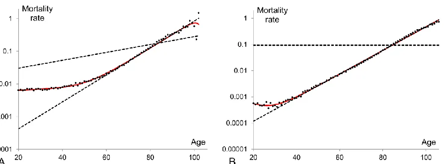
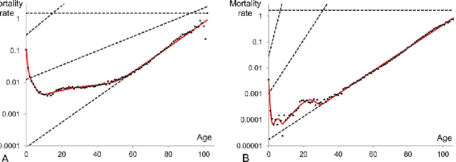
3 by a straight line. Graphically the actual mortality data generates patterns which have certain common features as well as some quantitative differences as compared to different cohorts and periods. A typical mortality pattern (Figure 1) originates from the initial mortality at age zero, falls down to a minimum point (approximately at the age of 10), increases to a local maximum (around the age of 25), then slightly decreases or remains constant and after the age of 35-40 advances exponentially satisfying the Gompertz law. At extreme old ages (above the age of 100) there is no common evidence on how the mortality curve behaves as the reported observations are controversial and provided with different explanations (Gavrilov and Gavrilova 2011; Greenwood and Irwin 1939; Olshansky 1998). Various statements made about the mortality dynamics at old ages include the mortality levelling-off or so-called “late-life mortality plateau” (Curtsinger and others 2006; Economos 1979; Mueller and Rose 1996), the late-life mortality deceleration (Depoid 1973; Gavrilov and Gavrilova 2001; Horiuchi and Wilmoth 1998; Thatcher and others 1998), the decline (Kannisto and others 1994; Vaupel and others 1998) or fluctuations at advanced ages (Avraam and others 2013).
The high initial level of mortality is due to the fact that new-borns are not particularly fit for the new environment they are born into and therefore, a relatively high proportion of them are not able to survive. As the forces of mortality due to environmental factors decrease, death rates decline. Mortality starts then to increase at the age of 10. One can state that mortality should increase exponentially from this age. However in actual mortality data the exponential increase of mortality is observable only after the ages of 35-40 (Figure 1) as between the ages 10 to 35 it overlaps with a local maximum on the mortality curve. This local maximum is apparent at the reproductive period of lifespan and is commonly called “the accidental hump” as it is related to the external causes of deaths (mainly accidents and maternal deaths) due to the risky behaviour of young adults.
Many studies have focused on the analysis of exponential increase of mortality in the range of ages 30 and above. By comparing parameters describing the exponential dynamics for data taken for different human societies it was found that in developed countries initial mortality, is lower while the mortality coefficient, is higher than these parameters describing data for less developed countries. This phenomenon, namely the inverse relationship between initial mortality and mortality coefficient appears to be fundamental (confirmed by all available data) and called the “compensation law” or “compensation effect” (Gavrilov and Gavrilova 1979;
0,
4 Gavrilov and Gavrilova 1991).
A number of mathematical models have been proposed to analyse mortality dynamics and explain its deviations from the exponential law at early and late life intervals. Some models postulate that a few different processes take place in the population and affect its mortality dynamics (Heligman and Pollard 1980; Thiele 1872), while others analyse the impact of population heterogeneity on the dynamics of mortality (Vaupel and others 1979; Vaupel and Yashin 1985). A model based on the assumption that the mortality dynamics is indeed underlined by an exponential law and deviations from this law are due to the heterogeneity of human populations has recently been proposed (Avraam and others 2013). It was shown that the observed age-specific mortality patterns can be reproduced in a model of heterogeneous population consisting of a few (up to four) subpopulations each following the exponential law over all ages.
Time evolution of mortality dynamics in human populations is of great scientific interest and has practical implementations especially for actuaries, who use extrapolation methods to project mortality trends in order to estimate future life expectancy (Booth and Tickle 2008; Pitacco 2004), and to price several longevity products. An example of mathematical study of this evolution can be found in (Gaille 2012), where the analysis of the evolution of the parameters of two conventional models (Heligman-Pollard and Lee-Carter) is used to forecast the Swiss mortality rates and to study the impact of longevity on Swiss pension funds. Mathematical analysis of the evolution of mortality dynamics could also be useful for demographers (to derive inferences on the population variance) and for biologists (to understand genetics underlying the evolutionary process of aging).
5 of the exponential law for all subpopulations are in line with the compensation law. Discussion of presented results is provided in Section 5.
2. Mathematical model and fitting procedure
In this work we use a previously proposed model (Avraam and others 2013) where a human population is considered as heterogeneous and composed of a number of subpopulations. The subpopulations are assumed to obey an exponential law, as given by equation (1), but differ in their mortality parameters (initial mortality, m0,and mortality coefficient, ). The mortality of the entire population is modelled as a mixture of weighted exponential terms. The weights represent the relative sizes (fractions) of the subpopulations; they depend on age and their sum is equal to unity at any age. Assuming that the entire population consists of subpopulations, the total mortality rate is expressed as:
where is the fraction or proportion representing the size, , of the j-th
subpopulation with respect to the whole population size, , at age , and is the exponential function for the j-th subpopulation with initial mortality and mortality coefficient Equation (2) expresses the mortality rate of the entire heterogeneous population at age within a cohort (with representing person-years, (Avraam and others 2013)) or time-period with the assumption that the population is stationary and its size and age-structure do not change over time.
Log-linear regression analysis is performed to fit the model given by equation (2) to mortality data. The Least Squares Method is used to estimate the free (unknown) parameters that minimize the sum of squared residuals (a residual is the difference between the theoretical and observed value). Bayesian Information Criterion (BIC) (Schwarz 1978) is used in order to select the optimal model, that is, to find the number of subpopulations in the model having the best fit to the dataset. The BIC is given by
x n 0 1 1 (2) j n n x
x jx jx jx j
j j
m m m e
1
/ n
jx jx jx
j
N N
Njx1 n jx j N
x mjx0 j m . j
6 where is the number of data points, is the sum of squared residuals divided by the number of data points and is the number of free parameters. The number of free parameters for
subpopulations is given by . The optimal model is the one with the lowest BIC.
3. Data
In this study we used two series of datasets. The first series represents the Swedish mortality (combined for males and females) for a period-interval of one century 1900 – 2000, provided by the Human Mortality Database (http://www.mortality.org). These datasets provide single age mortality rates resulting from all causes of death. The second series of datasets is from the World Health Organization (WHO), which maintains a comprehensive cause-of-death mortality database (http://www.who.int). This database provides the sizes of mid-year populations and number of deaths by cause for various countries over the last 50 to 60 years. We obtained data for Sweden (males’ population) from 1951 to 2010. The data are generally divided into five-year age-groups. Thus, our database is composed of nineteen groups, the first for infants less than one year old, a second for children aged one to four, thereafter in groups of five years, ending with the group aged 85 and above. The database of the WHO needs to be adjusted in order to analyse data consistently over time (proportional distribution of the number of deaths of unknown age; adjustments due to the changes of the International Classification of Diseases (ICD) over time (Table 1)). Details on these adjustments can be found in (Gaille and Sherris 2011) and (Arnold (-Gaille) and Sherris 2013). This database allows us to distinguish between extrinsic and intrinsic mortality.
To justify our interest in the relative impacts of intrinsic and extrinsic factors to mortality dynamics we refer to the original Gompertz work where he mentioned two different mortality groups: a first mortality group related to chance, without previous disposition to death or deterioration; a second mortality group referring to deterioration, or an increased inability to withstand destruction (Gompertz 1825). Today, the distinction is usually made between intrinsic and extrinsic causes of death, the intrinsic causes being related to Gompertz’s inability to oppose destruction. More specifically, the extrinsic causes of death represent external or environmental factors that produce death, while the intrinsic causes of death represent biological forces that lead
2
ˆ
ln( ) ln( ) (3)
d e d
BICn k n
d
n ˆe2
k
7 to death, namely aging or senescent (Carnes and Olshansky 1997; Makeham 1867; Shryock and others 1975). Makeham (Makeham 1867) suggested that the Gompertz law will fit much better with mortality due to biological causes (intrinsic causes). It is therefore interesting in our exponential modelling approach to apply our model to intrinsic causes of death. The extrinsic causes of death usually include the external causes of death (such as accidents, homicide and suicide) and the infectious and parasitic diseases, even if some studies recommend the inclusion of some other causes (see e.g. the classifications in (Carnes and others 2006)and a review in (Carnes and Olshansky 1997)). The WHO database allows us to analyse the mortality pattern excluding these extrinsic causes of death and then to focus on the mortality dynamics due to intrinsic mortality. Table 1 provides the ICD codes for the extrinsic causes we excluded.
4. Results
In this section we fit the model proposed in Section 2 to the data described in Section 3 in order to describe time-dependence of mortality patterns in terms of the evolution of the model parameters. In order to better capture the direction of the trend of each parameter over time, the evolution of each parameter is displayed with the most representative trendline within the examined time range. Two different monotonic functions (linear and exponential) are compared through the BIC (which, in the case of these two functions, works in the same way as R2) statistics. These two functions were chosen due to their interpretability with respect to the compensation effect of mortality, as further explained in the following sections.
8 and 4.6 respectively.
4.1 Evolution of mortality parameters for ages 40+
As mentioned earlier the exponential increase of mortality with age is evident in the mortality pattern at adulthood span after the reproductive period. It follows that the mortality data from age 40 are best fitted by a model of homogeneous population. Our analysis shows that at the beginning of the century, the data for ages 40+ slightly diverge from a pure exponential growth. An example is the 1900 period dataset shown in Figure 2A. For those data, the BIC
criterion indicates that a two-subpopulation model (BIC=-184.73) fits the data better than the homogeneous model (BIC=-164.08). On the other hand, more recent data indicate a stronger merge to the exponential growth and therefore the homogeneous model fits the data better than that involving two subpopulations. For example, the BIC numbers for homogeneous and two-subpopulation models fitting the data shown in Figure 2B are -319.88 and -319.07 respectively. It is therefore evident that the fit of the homogeneous model to the data for consecutive years gets better over time (one can read it by comparing panels A and B in Figure 2). This is mainly due to the extended impact that the accidental hump had on the mortality pattern at the beginning of the 20th century (Figure 2A). At that time the number of deaths caused by external factors, such as accidents, was considerably larger (as a result of poor education, inadequate transportation system, unsafe labour environment, lack of contraceptives, etc.) and therefore the accidental hump had a larger amplitude and impacted a wider age range. Over time the magnitude of the accidental hump decreased and at present it affects a smaller range of age groups. It is not surprising that some studies predict that the accidental hump will be less noticeable and even probably disappear in the coming years (Gaille 2012). Despite this observation, we only consider the model of homogeneous population (described by the exponential law) to fit the Swedish data from age 40 for consecutive years, in order to be consistent in our first step and to study the evolution of mortality parameters.
9 mortality coefficient a linearly increasing trend (Figure 3B). The decline of initial mortality is of no surprise, especially in developed countries where medicine and hygiene levels have improved rapidly over the last century. On the other hand the increase in the mortality coefficient is harder to explain. This phenomenon is known as the compensation law of mortality. This law states that a high initial mortality rate in a population is compensated with a low rate of mortality increase with age, or similarly a low initial mortality rate is compensated with a high rate of mortality increase with age (Gavrilov and Gavrilova 1979; Gavrilov and Gavrilova 1991; Gavrilov and Gavrilova 2006; Strehler 1978; Strehler and Mildvan 1960; Yashin and others 2000). The compensation law is also known as the “late-life mortality convergence”, because mortality trajectories between different populations converge to a specific point. The age at which the mortality trajectories converge is the age at which the last survivor dies and therefore we will call it “the target lifespan”. Similarly, the mortality at which the mortality trajectories converge will be called “the target mortality rate”.
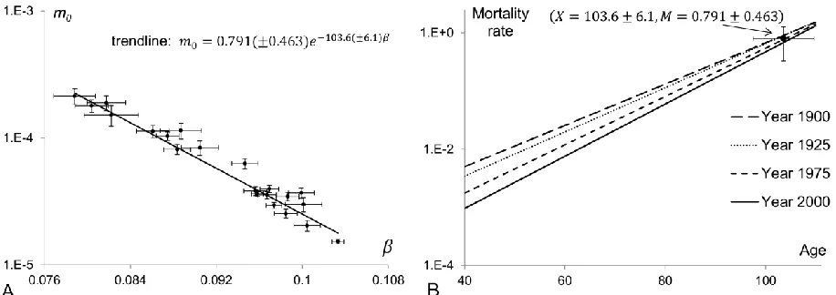
The inverse relationship between the mortality parameters of the modelled homogeneous population is shown in panel A of Figure 4. This plot confirms that a high initial rate of mortality is associated with a low mortality coefficient. It is apparent that there is a linear relationship between the logarithm of and parameter . This relationship, known as Strehler and Mildvan correlation, can be expressed mathematically as:
where X is the target lifespan and M is the target mortality rate (Gavrilov and Gavrilova 2006; Strehler 1978; Strehler and Mildvan 1960; Yashin and others 2000). From equation (4) it follows that if the mortality coefficient is an increasing linear function of time (like the trendline in Figure 3B), then the initial mortality declines exponentially (like the trendline in Figure 3A). It should be noted here that Strehler and Mildvan (Strehler and Mildvan 1960) used different notations and interpretations for the terms X and M but the essential meaning of the model was the same as above.
In panel B of Figure 4, the trajectories of the homogeneous model fitted to the Swedish data at four different years are plotted in the same semi-logarithmic plot. The mortality convergence is evident. The coordinates of the intersection point to which mortality trajectories are converging represent the target lifespan and target mortality rate. With a pure form of the compensation effect, all the exponential trajectories should cross that point. Even if the mortality
0
m
0
10 trajectories do not cross strictly at one specific point within the area formed around the error bars of the point ( ,X M), the compensation effect is still valid in its weak form. The error bars of X
and M represent the standard deviations of their values as estimated by the method described in (Reed 1989). The mortality trajectories that fit the Swedish data above age 40 for different years should theoretically intersect at the point (X 103.6 6.1, M 0.791 0.463) with a pure compensation effect. The coordinates (X and M) of this point define (as stated by equation (4)) the trendline (shown as a solid line) in panel A of Figure 4.
This first analysis showed that the compensation effect is evident in the Swedish population for ages above 40 when different periods are compared, although it is in its weak form. We are now interested in studying this effect for a wider age range and for heterogeneous populations, that is when a population is composed of a set of subpopulations.
4.2 Evolution of mortality parameters for ages 20+
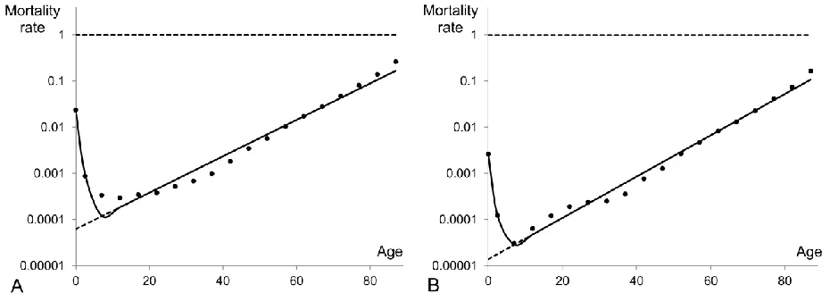
It appears that a two-subpopulation model is the best fit for Swedish mortality data which are cut at age 20. The mortality pattern above age 20 includes a part of the accidental hump (usually a piece of its right tail) and the exponential rise of mortality at older ages. There is a local minimum in between these two parts and therefore two subpopulations should be involved to reproduce the mortality pattern observed above age 20. Figure 5 presents examples of mortality data and fitted models for 1900 and 2000. The mortality dynamics of the two subpopulations are shown by dashed lines while the mortality of the entire population as calculated by equation (2) is shown by the red solid curve. The first subpopulation having higher initial mortality is frailer than the other and thus is producing decline in mortality at the right tail of the accidental hump while the second subpopulation is responsible for the exponential growth of the entire population mortality after the reproductive period. For clarity and consistency purposes, in the remaining part of this study the first subpopulation represents the one with the highest initial mortality level (j=1), the second is the one with the second highest initial mortality level (j=2), etc.
11 highest initial mortality) is still alive at that point. The mortality cross-section (or crossover as called in (Vaupel and Yashin 1985) occurs when one of the subpopulations has a lower mortality rate than the other subpopulation at younger ages, but higher at older ages. The two mortality trajectories of the subpopulations fitted to the Swedish 1900 period data (Figure 5A) cross each other at age 83, that is when 104 individuals of the first subpopulation (0.78% of the total population) are still alive at that age, while few of them remain alive at the local maximum age (age 98). For the 2000 period data (Figure 5B) the trajectories cross at age 84. The only individual of the frailest subpopulation alive at that age (0.002% of the total population at age 84) dies a couple of years after the point of intersection and therefore we don’t observe the decline of mortality at advanced ages on this panel. Another observation from Figure 5 is about the constant mortality of the frailest subpopulation in panel B. For that particular period, the frailest subpopulation with zero-slope ( ) appears to be optimal. This happens due to the constraint we set in the model, namely, that the mortality coefficients can’t be negative. Without this constraint the best fitted models can involve negative mortality coefficients, which means that the models incorporate a process opposite to senescence. Thus here and later, some of our best fits will have a mortality coefficient equal to zero for the frailest subpopulation.
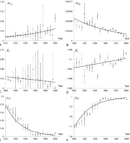
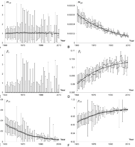
The time-evolution of mortality parameters in the model of a heterogeneous population fitted to the Swedish data for ages above 20 is shown in Figure 6. The initial mortality rate parameter and initial fraction of the first (frailest) subpopulation are shown in panels A, C and E respectively. Similarly the evolution of mortality parameters of the second (most robust) subpopulation is shown in panels B, D and F. Although the parameters are widely dispersed and presented results contain high standard errors, the shown trendlines reliably indicate the direction of trends.
Figure 6 indicates that the inverse relationship between the initial mortality rate and the mortality coefficient is observed for both subpopulations. We therefore conclude that the compensation law holds for each subpopulation, although in the first subpopulation it is reversed as compared to that in the second subpopulation. Indeed, in the most robust (second) subpopulation the initial mortality declines over time while its mortality coefficient increases (similar results as in Section 4.1). At the same time the initial mortality of the frailest (first) subpopulation increases while its mortality coefficient decreases.
1
0
10,
m
1
12 It is also interesting to note on Figure 6 that the frailest subpopulation shows an important volatility especially for more recent years, when this subpopulation does not considerably affect the population mortality pattern above age 20. Specifically, the fraction of the frailest subpopulation becomes very small (close to zero) from around 1960. Thus, the mortality of the entire population is mainly reflecting the mortality of the most robust subpopulation. The parameter values of the frailest subpopulation do not have an important impact on the entire population mortality schedule, and thus, a wide range of parameter values provides a good fit.
A new and interesting observation related to the structure of heterogeneous populations can be drawn from panels E and F in Figure 6. The fraction of the frailest subpopulation declines exponentially over time while the fraction of the most robust subpopulation increases accordingly. The frailest subpopulation represented 0.28% of the total population in 1900, while it only represented 0.03% in 2000. The population is then becoming more homogeneous over time. This important observation will be further discussed in the upcoming sections.
4.3 Evolution of mortality parameters for all ages excluding the
extrinsic causes of death
As mentioned in Section 3, the causes of death can be grouped into two categories: intrinsic and extrinsic. The intrinsic causes are related to the inability of biological organisms to oppose destruction. Makeham (Makeham 1867) suggested, among others, that the Gompertz law fits much better with mortality due to biological causes, this section focuses on the evolution of mortality due to intrinsic causes. Since the extrinsic causes of death include the external causes of death, the local maximum in the adulthood period (at approximately age 20 for the Swedish data in Figure 1), that is, the accidental hump is removed. Results in this section are based on mortality rates for Swedish males found on the WHO website, as mentioned in Section 3.
Figure 7 presents observed Swedish male mortality (dots) excluding extrinsic causes of deaths for the periods 1951 (panel A) and 2010 (panel B). The high level of infant mortality reflects mainly the deaths due to severe birth defects, malformations, preterm births, the sudden infant death syndrome, etc. Therefore the mortality trajectory drops down to a minimum point and after the age of 10 increases exponentially. Thus, by excluding the accidental hump we
10
20
13 observe that the exponential rise of mortality becomes apparent at the early stage of human life, just after age 10, and the pattern of mortality has a single minimum at that age. Therefore, a model of a heterogeneous population composed of two subpopulations should be sufficient to reproduce the actual data. Our studies show that a two-subpopulation model is indeed commonly a best fit for these data, although in some cases BIC values indicate that three-subpopulation models are more accurate. In this section we will fit all the consecutive periods with the two-subpopulation model for consistency. In the two-two-subpopulation model (see Figure 7), the mortality dynamics of the first subpopulation explains the high infant mortality and the mortality decline at young ages, while the second subpopulation describes the exponential rise of mortality after the age of 10.
The second subpopulation represents a bigger proportion of the total population than the first subpopulation. The first subpopulation has usually a zero-slope coefficient and a high initial mortality, close to 1. Thus, the first-subpopulation individuals die at the very young ages due to the high level of initial mortality. By the age of 10, the first subpopulation is completely eliminated. Consequently, after the age of 10, the mortality rate of the entire population increases exponentially according to the mortality dynamics of the second subpopulation.
The time evolution of parameters of the two-subpopulation model is shown in Figure 8. The fitted model parameters are presented with circle points with error bars, while the solid lines represent trendlines. We found that while the model parameters and describing the first subpopulation do not show any trend, the evolution of the other model parameters follows a trend. Although the estimation of model parameters comes with considerably large error bars the trendlines can be reliably approximated by linear or exponential functions. The frailest subpopulation has a zero-constant mortality coefficient (Figure 8C) and an approximately constant (slightly decreasing) initial mortality (Figure 8A). The second subpopulation has an exponentially decreasing initial mortality (Figure 8B) and an exponentially increasing mortality coefficient (Figure 8D). The fraction of the first subpopulation declines exponentially over time (Figure 8E), while the fraction of the second subpopulation is increasing accordingly (Figure 8F). The first subpopulation can be considered as static, with a constant initial mortality and a constant mortality coefficient. Only its proportion to the entire population is changing over time. An analysis of the compensation effect requires then an analysis of the mortality dynamics for the second subpopulation only.
10
14 Similarly to the case of the 20+ data shown in Figure 6 we observe the decline of the initial mortality rate of the second (most robust) subpopulation and the increase of its parameter and thus the inverse relationship between the two parameters is again observed, reflecting the compensation law of mortality.
As in the previous section, the heterogeneity in human populations is decreasing. The fraction declines over time and tends to zero while the fraction converges to 1. This could be interpreted as a reduction in the number of vulnerable new-borns who fail to survive in the new environment. This reduction can be viewed as a consequence of hygiene, medical and lifestyle improvements, etc. Since these individuals are no longer affected by fatal diseases at early ages, they are transferred to the most robust subpopulation and thus add to the mortality dynamics in the same way as other individuals in the most robust subpopulation.
The decrease in human heterogeneity leads to a very interesting observation: the decline in mortality rates of the entire population is partly due to the decreasing proportion of the population related to the first subpopulation. Indeed, the change over time in the structure of the population, that is the change in the fractions of the first and second subpopulations, explains most of the mortality decline of the entire population. Most of the past mortality decline is thus not due to a decline in the mortality of each subpopulation (reflected with changes in the mortality parameters), but due to a change in the structure of the population. This result will be further discussed in the following sections.
4.4 Evolution of mortality parameters for all ages including all
causes of death
In this section we will consider the model of heterogeneous populations as fitted to the mortality data on the entire age range including all causes of death. Swedish data for 1900-2000 have been used, as in Sections 4.1 and 4.2. According to BIC values a model consisting of four subpopulations is typically a best fit for these data (Avraam and others 2013). Figure 9 shows the fitted model for the first and the last periods under observation, that are 1900 (panel A) and 2000 (panel B).
The first subpopulation (with the highest initial mortality) describes the high infant mortality of the entire population and the deep mortality decline over the first few years. The second subpopulation has an impact on mortality in the age range from two (when first
10
15 subpopulation is almost gone) to 10 when this subpopulation has also practically vanished. The third subpopulation describes the accidental hump which occurs due to the accidental mortality for young adult males and the accidental in addition to maternal mortality for young adult females. The last subpopulation (with the lowest initial mortality but the biggest initial size) explains the exponential mortality trajectory of the entire population after the reproductive period.
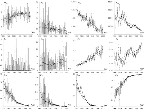
Figure 9 illustrates that the parameters of the four subpopulations are changing over time. Indeed, the points of intersections and the slopes of the dashed lines are different in panels A and B. Details are provided in Figure 10, where the time evolution of each parameter is shown. The plot has four columns, each column presenting the parameters of one subpopulation.
Figure 10 shows that the initial mortality of the first subpopulation increases while the initial mortalities of the other three subpopulations decrease over time (provided linear trends are not particularly accurate but confidently indicate the increasing/decreasing behaviour of data). The mortality coefficient of the first subpopulation (parameter ) is zero for almost all years. Since the parameter only affects the first few years of life, its value does not significantly influence the mortality pattern of the entire population (any value of the mortality coefficient combined with high level of initial mortality can reproduce the sharp initial decline of the mortality pattern). The mortality coefficients of the other three subpopulations (parameters
and ) increase (approximately linearly) over time, which (taking into account the decrease in the initial mortality) confirms the validity of the compensation law of mortality for the last three subpopulations. Figure 10 also reveals a very interesting observation, namely damped oscillations of initial mortality, , and mortality coefficient, , for the fourth subpopulation. These oscillations can reflect the effect of periodically changing external (e.g. climatic) factors on the mortality of the population, while their damping may indicate the evolution of the population’s resistance to these factors. Finally, the homogenisation effect is also shown in Figure 10. As in previous sections, the most robust subpopulation (fourth subpopulation) is continuously growing and becoming a more important fraction of the total population, while the initial fractions of the first three subpopulations decline exponentially over time. At the year 1900, the proportion of the main subpopulation was 67% of the total population while this proportion increased to 99% in the year 2000.
1
1
2,
3
440
16
4.5 Compensation effect
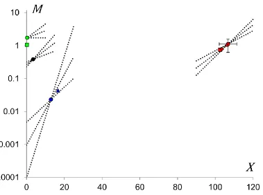
The inverse relationship between the time evolution of the initial mortality and the time evolution of the mortality coefficient was observed in previous sections for most subpopulations. A complementary phenomenon is the convergence of the mortality trajectories for each subpopulation. This convergence is manifested by the intersection of mortality trajectories (see Figure 4B) which, in the ideal case (a pure form of compensation effect), takes place in the same point for all trajectories, the coordinates of this point giving the target lifespan and target mortality, i.e. the age and the level of mortality at which the last survivors in the subpopulation of interest die (Gavrilov and Gavrilova 1979; Gavrilov and Gavrilova 1991; Gavrilov and Gavrilova 2006; Strehler 1978; Strehler and Mildvan 1960; Yashin and others 2000). The target lifespans for the individuals of each subpopulation are found through the Strehler and Mildvan correlation (equation 4). The target lifespans resulting from the preceding four sections are estimated as:
1. For homogeneous population fitting the Swedish data above age 40 (Section 4.1): 103.6 years;
2. Two subpopulations reproducing the Swedish mortality patterns for ages above 20 (Section 4.2): 16.7 and 106 years respectively;
3. Two subpopulations reproducing the Swedish male mortality patterns excluding the extrinsic mortality (Section 4.3): 0.2 and 102.6 years respectively;
4. Four subpopulations representing Swedish entire mortality schedule (Section 4.4): 0.3, 3.5, 12.9 and 106.8 years respectively.
17 it has the same colour (blue) as the point for the third subpopulation of the four-subpopulation model which is also responsible for the accidental hump. Similarly the lifespan of the first subpopulation, reflecting the Swedish male mortality excluding the extrinsic causes of death, explains the sharp initial decline in the mortality pattern, and thus the intersection point for it has the same colour (green) as the point for the first subpopulation in the four-subpopulation model for Swedish mortality (green square and green circle points respectively in Figure 11). Finally the red colour represents the exponential rise of mortality after sexual maturity and thus the homogeneous population representing the Swedish mortality for age 40 and above is shown by the red rhombus, the second subpopulation of the model representing the Swedish mortality at age 20+ is shown by the red triangle, while the second subpopulation reflecting the Swedish male mortality excluding the extrinsic causes of death is represented by the red square point, and the fourth subpopulation in the four-subpopulation model is presented by a red circle point. Samples of hypothetical mortality dynamics for each subpopulation of the four-subpopulation model are given by dashed lines.
The most interesting observation from Figure 11 is that the markers of the same colour are located close to each other. Thus, the four models studied in Sections 4.1-4.4, even if they were applied to different age ranges and datasets, provide similar results by indicating the existence of almost identical subpopulations. Therefore, the target lifespan for the total population in Sweden is reflected through the target lifespan for the most robust subpopulation (which appears in all four models) and thus lies between ages 102 and 107.
4.6 The role of homogenization in the evolution of mortality
dynamics
18 reduction of mortality within one century is a result of
1. the alteration in population structure, that are changes in subpopulation’s fractions, especially at young ages (difference between solid red and dashed blue curves in Figure 12) and
2. the alteration of the exponential dynamics of the subpopulations, that are changes in initial mortalities, and mortality coefficients, (difference between dashed blue and solid blue curves in Figure 12).
Looking at Figure 12 we can also conclude that the decrease in mortality at younger ages is mostly due to the homogenization of the population while at older ages is entirely due to changes in the mortality parameters of the most robust subpopulation.
5. Discussion and Conclusion
Investigations of human mortality dynamics have practical implementations as they may help to find ways to increase our lifespan. These investigations also have a fundamental value as they help to understand biological processes and genetics underlying the process of aging. One of the important ways to conduct such investigations is represented by mathematical modelling. Various assumptions have to be made to design a mathematical model, especially if one aims to model all relevant features observed in the mortality pattern of the entire lifespan. One of the commonly used assumptions is that a population is heterogeneous and composed of several subpopulations having different mortality dynamics (Rossolini and Piantanelli 2001; Vaupel 2010). The possible interpretation of the model parameters is extremely important to conduct deeper analyses and for forecasting purposes (Booth and Tickle 2008). The time evolution of the parameters of a model fitted to several observed periods provides then important insights in potential future evolutions. Such studies have been performed using various models of mortality dynamics (Bell 1997; Felipe and others 2002; Gaille 2012; Gaille and Sherris 2011; Lee and Carter 1992; McNown and Rogers 1989; McNown and Rogers 1992; Njenga and Sherris 2011; Tabeau and others 2001).
In this work we have analysed the evolution of the parameters in a model of heterogeneity of human populations where each subpopulation follows an exponential law of mortality (Avraam and others 2013). We fitted the model to four different datasets. First, the
0
j
19 homogeneous exponential law was fitted to Swedish mortality rates for ages above 40 for the periods 1900 to 2000. Second, the model of heterogeneous population with two subpopulations was fitted to the Swedish mortality rates for ages 20 plus. Third, the two-subpopulation model was fitted to Swedish male mortality rates over the entire lifespan, excluding deaths due to extrinsic factors, for the periods 1951 to 2010. Fourth, the model of heterogeneous population with four subpopulations was fitted to the entire lifespan dataset of the Swedish population for the periods 1900-2000. Our model fitting approach results in four main findings.
The first remarkable observation concerns the model used, that is the best fit to the mortality dynamics for the most complete mortality data is given by the four-subpopulation model. The novel result associated with this model is given by the second subpopulation which distinguishes the impact of child mortality from infant mortality to the entire mortality pattern. Occurrence of the subpopulation which counts for the child mortality makes our model different from other notable models (such as Heligman-Pollard) where the mortality dynamics is commonly decomposed to only three stages corresponding to early childhood, accidental mortality and late-life adulthood.
Second, our model does not capture the “late-life mortality plateau” which was reported by many researches as described in the introduction. We have fitted the model to each year within 20th century and only a few of the fits have captured the mortality deceleration at older ages. It turns out that the deviations in mortality dynamics from the exponential increase at older ages are not always significant enough to be captured by our model. As we use the BIC for evaluation of how the model fits the data, the best fit becomes very sensitive to the number of subpopulations in the model. For example five-subpopulation model is worse than four-subpopulation as it has more model parameters although in terms of standard error it fits data better. To analyse the dynamics of mortality at old ages it is more appropriate to consider a shorter range of ages for example 80+. We have checked and confirm that the best fit for this range of ages is commonly given by two subpopulations and the model reproduces mortality deceleration around the age of 100.
20 approximately constant initial mortality and a constant mortality coefficient. The frailest subpopulation, namely the subpopulation with the highest initial mortality rate, represents a small proportion of the entire population and disappears after a couple of years (the individuals belonging to that subpopulation die a few years after their birth). Therefore, except for the very young ages, this subpopulation has a negligible impact on the mortality pattern. It is also interesting to note by comparing Figures 6 and 8 that the evolution of the parameters of the two-subpopulation model for ages above 20 (Section 4.2) is similar in many ways to the evolution of the parameters of the two-subpopulation model excluding the extrinsic causes of death (Section 4.3). It is related to the fact that in both models, the most robust subpopulation explains the exponential rise of mortality over the adulthood period in the entire population and the frailest subpopulation describes a decline in the mortality pattern at young ages. Indeed, in the two-subpopulation model for ages 20+, the frailest two-subpopulation represents the decline forming the right tail of the accidental hump (Figure 5), while in the two-subpopulation model excluding extrinsic mortality, the frailest subpopulation is responsible for the initial decline of mortality at very young ages (Figure 7).
Our forth main finding is the homogenization of the population over time. Indeed, we have shown that the fractions of all subpopulations except for the most robust decline over time. We have found that the fraction of the most robust subpopulation gradually increases being equivalent to 67% of the total population in 1900 and 99% in 2000 for the Swedish data. The homogenisation we report here is related to the evolution of mortality in developed countries and does not directly reflect the variations in genotype in the population. It rather reflects the fact that in course of time, with improvements in medical service and life conditions, the variations in genotype of people become less important in terms of their duration of life. Contemporary genetic studies (Cavalli-Sforza and Feldman 2003) indicate that the genetic variability in human populations is increasing over time. This increase is rather explained by the fact that the mortality is gradually reducing and therefore not all of those who recently survive and give offspring (i.e. bring diversity into a gene pool) would be able to do so in the past.
21 subpopulations (decline from the blue dashed curve to the blue solid curve in Figure 12), which is reflected with a change in the mortality parameters of each subpopulation. The implications are remarkably important for potential future mortality improvements: once the homogenization process is over, that is the mortality of the entire population will only reflect the mortality of the healthiest subpopulation, the potential for future decrease in mortality will be relatively small compared to what we observed over the last century. New developments in mortality forecasting approaches should consider this aspect to avoid overestimation of future mortality improvements.
To conclude, the above findings can be used in a future work to further enhance our methodological approach. It would be of great interest to fit a mortality surface (rather than a line) over the plane given by two variables: age and time. Fitting a surface is a difficult task requiring further assumptions about its structure. This structure can now be postulated as based on the assumptions that the evolutions of initial mortality, m0, is represented by a linear function while the evolution of mortality coefficient, , by an exponent. This approach would allow us to obtain further results on the mortality structure of human populations, and thus could confirm, enhance and develop further the results presented here.
Acknowledgements
This work has been supported by the BBSRC grant BB/K002430/1 to BV. The authors declare no competing financial interests.
References
Addison, J. The vision of Mirza. Spectator. 159; 1711
Arnold (-Gaille), S.; Sherris, M. Forecasting Mortality Trends Allowing for Cause-of-Death Mortality Dependence. North American Actuarial Journal. 17:273-282; 2013
Avraam, D.; de Magalhaes, J.P.; Vasiev, B. A mathematical model of mortality dynamics across the lifespan combining heterogeneity and stochastic effects. Exp Gerontol. 48:801-811; 2013
Bell, W.R. Comparing and assessing time series methods for forecasting age-specific fertility and mortality rates. J Off Stat. 13:279-303; 1997
Booth, H.; Tickle, L. Mortality Modelling and Forecasting: a Review of Methods. Annals of Actuarial Science. 3:3-43; 2008
Carnes, B.A.; Holden, L.R.; Olshansky, S.J.; Witten, M.T.; Siegel, J.S. Mortality partitions and their relevance to research on senescence. Biogerontology. 7:183-198; 2006
22 32:615-631; 1997
Cavalli-Sforza, L.L.; Feldman, M.W. The application of molecular genetic approaches to the study of human evolution. Nature genetics. 33 Suppl:266-275; 2003
Curtsinger, J.W.; Gavrilova, N.S.; Gavrilov, L.A. Biodemography of aging and age-specific mortality in Drosophila melanogaster. Handbook of the biology of aging. Amsterdam: Elsevier Academic Press; 2006
Depoid, F. Mortality of old people over 85. Population. 28:755-792; 1973
Economos, A.C. A non-Gompertzian paradigm for mortality kinetics of metazoan animals and failure kinetics of manufactured products. Age. 2:74-76; 1979
Felipe, A.; Guillen, M.; Perez-Marin, A.M. Recent mortality trends in the Spanish population. British Actuarial Journal. 8:757-786; 2002
Gaille, S. Forecasting mortality: when academia meets practice. Eur Actuar J. 2:49-76; 2012 Gaille, S.; Sherris, M. Modelling mortality with common stochastic long-run trends. Geneva Pap
Risk Insur-Issues Pract. 36:595-621; 2011
Gavrilov, L.A.; Gavrilova, N.S. Determination of species length of life. Doklady Akademii Nauk SSSR: Biological Sciences. 246:905-908; 1979
Gavrilov, L.A.; Gavrilova, N.S. The Biology of Life Span: A Quantitative Approach. New York: Harwood Academic Publisher; 1991
Gavrilov, L.A.; Gavrilova, N.S. The reliability theory of aging and longevity. J Theor Biol. 213:527-545; 2001
Gavrilov, L.A.; Gavrilova, N.S. Reliability Theory of Aging and Longevity. in: Masoro E.J., Austad S.N., eds. Handbook of the Biology of Aging. San Diego, CA, USA: Elsevier Academic Press; 2006
Gavrilov, L.A.; Gavrilova, N.S. Mortality measurement at advanced ages: A study of the Social Security Administration Death Master File. North American actuarial journal : NAAJ. 15:432-447; 2011
Gompertz, B. On the Nature of the Function Expressive of the Law of Human Mortality, and on a New Mode of Determining the Value of Life Contingencies. Philosophical Transactions of the Royal Society of London. 115:513-583; 1825
Greenwood, M.; Irwin, J.O. The Biostatistics of Senility. Human Biology. 11:1-23; 1939
Heligman, L.; Pollard, J.H. The age pattern of mortality. Journal of the Institute of Actuaries. 107:49-80; 1980
Horiuchi, S.; Wilmoth, J.R. Deceleration in the age pattern of mortality at older ages. Demography. 35:391-412; 1998
Kannisto, V.; Lauritsen, J.; Thatcher, A.R.; Vaupel, J.W. Reductions in Mortality at Advanced Ages: Several Decades of Evidence from 27 Countries. Population and Development Review. 20:793-810; 1994
Lee, R.D.; Carter, L.R. Modeling and Forecasting U. S. Mortality. Journal of the American Statistical Association. 87:659-671; 1992
Makeham, W.M. On the Law of Mortality. Journal of the Institute of Actuaries. 13:325-358; 1867
McNown, R.; Rogers, A. Forecasting Mortality: A Parameterized Time Series Approach. Demography. 26:645-660; 1989
McNown, R.; Rogers, A. Forecasting cause-specific mortality using time series methods. International Journal of Forecasting. 8:413-432; 1992
23 Acad Sci U S A. 93:15249-15253; 1996
Njenga, C.N.; Sherris, M. Longevity risk and the econometric analysis of mortality trends and volatility. Asia-Pacific Journal of Risk and Insurance. 5:22-73; 2011
Olshansky, S.J. On the biodemography of aging: a review essay. Population and Development Review. 24:381-393; 1998
Pearson, K. The chances of death and other studies in evolution. London: Edward Arnold; 1897 Pitacco, E. From Halley to “frailty”: a review of survival models for actuarial calculations.
Giornale dell’Istituto Italiano degli Attuari. 67:17-47; 2004
Reed, B.C. Linear least-squares fits with errors in both coordinates. American Journal of Physics. 57:642-646; 1989
Rossolini, G.; Piantanelli, L. Mathematical modeling of the aging processes and the mechanisms of mortality: paramount role of heterogeneity. Exp Gerontol. 36:1277-1288; 2001
Schwarz, G. Estimating the dimension of a model. Ann Stat. 6:461-464; 1978
Shryock, H.S.; Siegel, J.S.; Larmon, E.A. The methods and materials of demography. Washington, DC: U.S. Dept of Commerce, Bureau of the Census, U.S. Govt. Printing Office; 1975
Strehler, B.L. Time, cells, and aging. New York: Academic Press; 1978
Strehler, B.L.; Mildvan, A.S. General Theory of Mortality and Aging (A stochastic model relates observations on aging, physiologic decline, mortality and radiation). Science. 132:14-21; 1960
Tabeau, E.; van den Bergh Jeths, A.; Heathcote, C. Forecasting mortality in developed countries. Insights from a statistical, demographic and epidemiological perspective. Dordrecht: Kluwer Academic Press; 2001
Thatcher, A.R.; Kannisto, V.; Vaupel, J.W. The force of mortality at ages 80 to 120. Odense: Odense University Press; 1998
Thiele, P.N. On a mathematical formula to express the rate of mortality throughout the whole life. Journal of the Institute of Actuaries. 16:313-329; 1872
Turner, E.L.; Hanley, J.A. Cultural imagery and statistical models of the force of mortality: Addison, Gompertz and Pearson. J R Stat Soc Ser A. 173:483-499; 2010
Vaupel, J.W. Biodemography of human ageing. Nature. 464:536-542; 2010
Vaupel, J.W.; Carey, J.R.; Christensen, K.; Johnson, T.E.; Yashin, A.I.; Holm, N.V.; Iachine, I.A.; Kannisto, V.; Khazaeli, A.A.; Liedo, P.; Longo, V.D.; Zeng, Y.; Manton, K.G.; Curtsinger, J.W. Biodemographic trajectories of longevity. Science. 280:855-860; 1998
Vaupel, J.W.; Manton, K.G.; Stallard, E. The impact of heterogeneity in individual frailty on the dynamics of mortality. Demography. 16:439-454; 1979
Vaupel, J.W.; Yashin, A.I. The deviant dynamics of death in heterogeneous populations. Sociological Methodology:179-211; 1985
24
Figures and Figure Legends
Figure 1: Mortality rates for the Swedish population in the period 1900 (panel A) and 2000
(panel B) presented in a semi-logarithmic scale. The data are taken from the Human Mortality
Database, http://www.mortality.org.
Figure 2: Homogeneous model (solid line) fitted to the 1900 (panel A) and 2000 (panel B)
period Swedish data (dots) from age 40 and above. The mortality parameters as estimated by
the Least Squares Method are: for panel A and
for panel B.
0 0.000189,
m 0.0818 m0 0.000015,
[image:24.612.87.533.388.554.2]25
Figure 3: Evolution of the parameters of the homogeneous model fitted to the Swedish
mortality rates from age 40, for the periods 1900 to 2000 with five-year intervals. Panel A
shows an exponentially decreasing trend for the initial mortality and panel B - a linearly
increasing trend for the mortality coefficient. In both plots the parameters are presented by dots
and the trendlines by solid lines. Error bars represent the standard deviations of estimated
parameters.
Figure 4: Compensation effect in 40+ mortality dynamics. Panel A shows the inverse
relationship between the parameters of the fitted homogeneous model to the Swedish mortality
rates for ages 40+ for the period data in the interval 1900-2000. The relationship between the
logarithm of the initial mortality and the mortality coefficient is shown to be linear. Panel B
shows the convergence of the exponential functions fitted to the Swedish data for ages 40+ and
[image:25.612.81.535.69.232.2] [image:25.612.78.536.425.587.2]26
Figure 5: Heterogeneous model fitted to mortality data for ages 20+. A two-subpopulation
model is fitted to Swedish (males and females) data (dots) for the periods 1900 (panel A) and
2000 (panel B). Dashed lines represent the mortality rates of each subpopulation (exponential
functions) while the solid (red) curve is the mortality of the whole population as described by the
model of heterogeneous population. The model parameters as estimated by the Least Squares
Method are for panel A: 1st subpopulation and 2nd
subpopulation and for panel B: 1st subpopulation
and 2nd subpopulation
.
10 0.01742,
m
1
0.0278,
10 0.2841120 0.000063,
m
2
0.0951,
200.7158910 0.09361,
m
10,
100.03114 m200.000015,
2 0.10377,20 0.96886
[image:26.612.86.533.91.257.2]27
Figure 6: Evolution of the parameters of a two-subpopulation model fitted to the Swedish
mortality rates for ages 20+. Panels A, C and E show evolution of parameters (initial mortality
(m0), mortality coefficient (β) and initial fraction (ρ0)) associated with the first subpopulation
while the panels B, D and F – with the second.The circle points with error bars correspond to
the model parameters and their standard deviations as estimated by the Least Squares Method
[image:27.612.81.537.70.573.2]28
Figure 7: Heterogeneous model fitted to mortality data which exclude extrinsic causes of
death. A two-subpopulation model is fitted to Swedish male data (dots) for the periods 1951
(panel A) and 2010 (panel B). Dashed lines represent the mortality rates of each subpopulation
(exponential functions) while the solid curve is the mortality of the whole population as
described by the model of heterogeneous population. The model parameters as estimated by the
Least Squares Method are for panel A: 1st subpopulation
and 2nd subpopulation and for panel B: 1st
subpopulation and 2nd subpopulation
.
10 0.99013,
m
10, 10 0.03324 20 0.000062,m 2 0.0908, 200.96676 10 0.97567,
m
10, 100.00395 m20 0.000014,2 0.103,
[image:28.612.71.536.72.236.2]29
Figure 8: Evolution of the parameters of a two-subpopulation model fitted to the Swedish
male mortality rates for all ages and excluding extrinsic causes of death. Panels A, C and E
show evolution of parameters (initial mortality (m0), mortality coefficient (β) and initial fraction
(ρ0)) associated with the first subpopulation while the panels B, D and F – with the second.The
circle points (with error bars) give the model parameters as estimated by the Least Squares
[image:29.612.81.539.73.571.2]30
Figure 9: Heterogeneous model fitted to mortality data including extrinsic causes of death. A
four-subpopulation model is fitted to Swedish (males and females) mortality rates (dots) for the
periods 1900 (panel A) and 2000 (panel B). Dashed lines represent the mortality rates of each
subpopulation (exponential functions) while the red solid curve is the mortality of the whole
population as described by the model of heterogeneous population. The model parameters as
estimated by the Least Squares Method are for Panel A: 1st subpopulation
2nd subpopulation 3rd
subpopulation and 4th subpopulation
and for Panel B: 1st subpopulation
2nd subpopulation 3rd
subpopulation and 4th subpopulation
10 1.50935,
m
1 0,
100.09936, m20 0.31023,
2 0.10653, 20 0.0536,30 0.01229,
m
3 0.05188,
30 0.1792940 0.00009,
m
4 0.09065,
40 0.66775 m10 1.69434,1 0,
10 0.00331, m20 0.02771,
2 0.61132,
20 0.00028,30 0.00103,
m
3 0.23672, 30 0.004540 0.000017,
31
Figure 10: Evolution of the parameters of the four-subpopulation model fitted to Swedish
mortality for each year over the periods 1900-2000. Each of column shows evolution of
parameters (initial mortality (m0), mortality coefficient (β) and initial fraction (ρ0)) associated
with one of the subpopulation. The dot points (with error bars) give the model parameters as
estimated by the Least Squares Method and the solid curves show trendlines for the evolution of
[image:31.612.76.540.69.425.2]32
Figure 11: Compensation effect in heterogeneous models. The coordinates of coloured markers
give the target lifespan and target mortality for each subpopulation of each model considered in
sections 4.1-4.4.The rhombus (red) marker corresponds to the homogeneous population fitted to
the Swedish mortality from age 40 and above. The two triangle markers (red and blue)
correspond to the subpopulations of the two-subpopulation model representing the Swedish
mortality from age 20 and above. The two square markers (red and green) correspond to the
subpopulations of the two-subpopulation model fitted to the Swedish male mortality excluding
the extrinsic causes of death. The four circle markers correspond to the four subpopulations of
the model fitted to the entire Swedish dataset. The colour used to draw a marker is the same for
the subpopulations in different models having an impact in the same age interval: green is for
infant mortality, black for child mortality, blue for the accidental hump and red for the
exponential growth of mortality after the reproductive period. Error bars representing the
standard deviations for the coordinates of the marker representing the most robust subpopulation
in four-subpopulation model are shown. Error bars for the three other subpopulations of this
model cannot be shown since they are smaller than the size of markers used in the figure. Sample
mortality trajectories are presented in each intersection point of the four-subpopulation model to
33
Figure 12: Reduction in the Swedish mortality rates within one century (from 1900 to 2000).
The patterns formed by the four-subpopulation model fitted to the 1900 (red solid curve) and
2000 (blue solid curve) Swedish mortality rates are plotted in a semi-logarithmic plot. The
dashed blue curve indicates an artificial pattern formed by the four-subpopulation model with
the initial mortalities and mortality coefficients estimated by fitting the 1900 period data and the