The parametric characteristics of frequency response functions for nonlinear systems

This is a repository copy of The parametric characteristics of frequency response functions for nonlinear systems.

White Rose Research Online URL for this paper: http://eprints.whiterose.ac.uk/74592/

Monograph:

Jing, X.J., Lang, Z.Q., Billings, S.A. et al. (1 more author) (2006) The parametric

characteristics of frequency response functions for nonlinear systems. Research Report. ACSE Research Report no. 932 . Automatic Control and Systems Engineering, University of Sheffield

Reuse

Unless indicated otherwise, fulltext items are protected by copyright with all rights reserved. The copyright exception in section 29 of the Copyright, Designs and Patents Act 1988 allows the making of a single copy solely for the purpose of non-commercial research or private study within the limits of fair dealing. The publisher or other rights-holder may allow further reproduction and re-use of this version - refer to the White Rose Research Online record for this item. Where records identify the publisher as the copyright holder, users can verify any specific terms of use on the publisher’s website.

Takedown

If you consider content in White Rose Research Online to be in breach of UK law, please notify us by

The Parametric Characteristics

of Frequency Response Functions for

Nonlinear Systems

X. J. Jing, Z. Q. Lang, S. A. Billings, and G. R. Tomlinson

Department of Automatic Control and Systems Engineering The University of Sheffield

Mappin Street, Sheffield S1 3JD, UK

The Parametric Characteristics of Frequency

Response Functions for Nonlinear Systems

Xing-Jian Jing1, Zi-Qiang Lang1, Stephen A. Billings1 and Geofrey R. Tomlinson2

1 Department of Automatic Control and Systems Engineering, University of Sheffield 2 Department of Machenical Engineering, University of Sheffield

Mappin Street, Sheffield, S1 3JD, U.K.

{X.J.Jing, Z.Lang, S.Billings & g.tomlinson}@sheffield.ac.uk

Abstract: The characteristics of the frequency response functions of nonlinear systems can be revealed and analyzed through the analysis of the parametric characteristics of these functions. To achieve these objectives, a new operator is defined, and several fundamental and important results about the parametric characteristics of the frequency response functions of nonlinear systems are developed. These theoretical results provide a significant and novel insight into the frequency domain characteristics of nonlinear systems and circumvent a large amount of complicated integral and symbolic calculations which have previously been required to perform nonlinear system frequency domain analysis. Several new results for the analysis and synthesis of nonlinear systems are also developed. Examples are included to illustrate potential applications of the new results.

1

Introductions

Nonlinear systems are far more complex than linear systems, and can exhibit harmonics, complex inter-modulations and even chaos (Pearson 1994). In order to understand and unravel these complicated phenomena, many authors have studied the analysis of nonlinear systems in both the time domain and the frequency domain (Graham and McRuer 1961, Sastry 1999, Chua and Ng 1979, Rugh 1981).

characteristics of nonlinear systems were studied, respectively. The bound characteristics of the frequency response functions and energy transfer characteristics have also been studied and discussed (Zhang and Billings 1996, Billings and Lang 1996, Lang and Billings 2005).

Although significant results have been achieved, many problems remain unsolved regarding the characteristics of the GFRFs and the system output frequency response function, including how the frequency response functions are influenced by the parameters of the underlying system, and the connection to complex non-linear behaviours. The GFRFs are actually a sequence of multivariable functions defined in a high dimensional frequency space. The evaluation of the values of the GFRFs higher than fourth or fifth order can become hard due to the large amount of algebra or symbolic manipulations that are involved (Yue et al. 2005). Moreover, existing recursive algorithms for the computation of the GFRFs do not explicitly and simply reveal the analytical relationship between the time domain system model parameters and the system frequency response functions in a clear and straightforward manner. These inhibit the practical application of the existing theoretical results to a certain extent. Therefore, the development of new methods to circumvent the computational complexity and to more clearly reveal the characteristics of the frequency response functions is of great importance for the analysis and synthesis of nonlinear systems.

Previous results (Peyton-Jones and Billings 1989) show that for the NARX model the recursive computation procedure for the GFRFs involves the contribution of different model parameters to the system nonlinear characteristics of different orders. Hence, an alternative approach to analyse the characteristics of the frequency response functions and the effects of different types of nonlinearities on the system would involve study of the characteristics of the system model parameters on the frequency response functions. Therefore, a novel and effective coefficient extraction operator is defined in this paper. Using this new operator, several fundamental results relating to the parametric characteristics of the frequency response functions for nonlinear systems are derived. The parametric characteristics of the GFRFs and the system output spectrum can easily be achieved using a recursive algorithm which uses the system time domain model parameters without the need to determine individual GFRFs. The results reveal the explicit relationship between the system time domain model parameters and the system frequency response functions, and provide a significant and novel insight into the frequency domain characteristics of nonlinear systems. Important characteristics of the frequency response functions of nonlinear systems are also revealed and analyzed based on the new parametric method. The new results derived in the present study provide a new and effective approach which should be very useful for the analysis and synthesis of nonlinear systems in the frequency domain.

2

Frequency response functions of nonlinear systems

∑

∫

∫

∏

=

∞ ∞

− ₌

∞ ∞

− −

= N

n

n

i

i i n

n ut d

h t

y

1 1

1, , ) ( )

( )

( L τ Lτ τ τ (1) where N is the maximum order of the series, and h_n(τ₁,L,τ_n)is a real valued function of

n

τ

τ₁,L, which is referred to as the nth order Volterra kernel. The frequency domain input-output description of the system can be obtained as (Lang and Billings 1996)

∑

∫

∏

= − + + = =

= N

n

n

i

i n

n n

n

d j U j

j H n

j Y

1 1

1 1

1

) ( ) , , ( )

2 (

1 )

(

ω ω ω

ω σ ω ω

ω π

ω

L

L (2) where,

∫

∫

−∞∞

∞ ∞

− − + +

= n n n n n

n

n j j h j d d

H ( ω1,L, ω ) L (τ1,L,τ )exp( (ω1τ1 L ωτ )) τ1L τ (3)

is known as the nth order Generalized Frequency Response Function(GFRF).

When the system input is a multi-tone function described by

∑

=

∠ + = K

i

i i

i t F

F t

u

1

) cos(

)

( ω (4) The system output frequency response function can be described as (Lang and Billings, 1996):

∑

∑

= + + =

= N

n

k k

k k

n n

n k k

n

n F F

j j

H j

Y

1 ₁

1

1, , ) ( ) ( ) (

2 1 ) (

ω ω ω

ω ω

ω ω

ω

L

L

L (5)

where,

{

}

⎪⎩ ⎪ ⎨

⎧ ∈ =± ±

= ∠

else 0

, , 1 , if

)

( F e k K

F k

F j i

i ω ω L

ω .

The GFRFs in (3) for specific and simple nonlinear models can be derived by using the probing method in Rugh (1981). Consider the nonlinear systems which can be described by the Nonlinear AutoRegressive model with eXogenous input (NARX)

∑ ∑

∏

∏

∑

= =

+

+ = =

+ =

+

− −

= =

m

p K

k k

q p

p i

i p

i

i q

p q

p m

M

m m

q p

k t u k t y k

k c t

y

t y t y

0 , 1 1 1

1 , 1

1

) ( ) ( ) , , ( )

(

) ( )

(

L

(6)

where, ym(t) is the mth-order output of the system, and p+q=m, ki=1,…, K,

∑

∑

∑

= =

= +

+

⋅ ⋅

=

⋅ K

k K

k K

k

k, pq 1 1 pq 1

) ( ) ( ) (

1 1

L .

Nonlinear system (6) represents a wide class of nonlinear systems and includes several well known nonlinear input-output models as special cases (Chen and Billings 1989). In this model, the parameters such as c0,1(.) and c1,0(.) represent the linear system parameters

corresponding to the linear terms in the model such as y(t-1) or u(t-2) etc, and all other parameters represent the nonlinear system parameters. p+q is referred to as the nonlinear degree of the nonlinear parameterc_pq(⋅). A nonlinear parameter c_pq(⋅)corresponds to a

nonlinear term in the model of the p+qth degree of the form

∏

∏

+

+ = =

−

− p q

p i

i p

i

i u t k

k t y

1 1

) ( )

q

p_{u t}

t

y( −1) ( −2) . Obviously, when p+q =1, the corresponding parameters are associated with the linear model terms. Let

⎟ ⎟ ⎟ ⎠ ⎞ ⎜ ⎜ ⎜ ⎝ ⎛ + = = = = + = = ₊ q p i K k M m m q p m p k k c K M C i q p pq L L L L L 1 , 1 1 , , 0 ) , , ( ) ,

( ₁ (7)

which includes all the parameters of the model (6).

For the NARX model in (6), the following recursive algorithm was derived by Peyton-Jones and Billings (1989) to compute the GFRFs:

∑ ∑

∑∑ ∑

∑

= = − = − = = − − + + + − + − + = + + + − + + + − = ⋅ + n p K k k n p n p p n q q n p K k k q n p q n q p q p q n q n q p q p K k k n n n n n n p q p n j j H k k c j j H k k j k k c k k j k k c j j H n L

2 , 1

1 , 1 0 , 1

1 1 , 1

1 , 1 1 1 , 1 , 1 1 1 , 0 1 1 1 1 ) , , ( ) , , ( ) , , ( )) ( exp( ) , , ( )) ( exp( ) , , ( ) , , ( ) ( ω ω ω ω ω ω ω ω ω ω L L L L L L L L (8)

∑

− + = − − + + + − = ⋅ 1 1 1 1 1 , 1

, () ( , , ) ( , , )exp( ( ) )

p n i p i n i p i n i i p

n H j j H j j j k

H ω L ω ω L ω ω L ω (9)

) ) ( exp( ) , , ( ) , ,

( _{1 1 1 1}

1

, j j H j j j k

H_n ω L ω_n = _n ω L ω_n − ω +L+ω_n (10) where L(n)=

∑

= + + − − K k n k j k c 1 1 1 1 0 , 1 1 ) ) ( exp( ) (

1 ω L ω . Moreover, Hn,p(jω1,L,jωn) in (9) can also be

rewritten as

∑ ∏

− + == = ∑ + + − = + + + + 1 1 1 1 , 1 1

1, , )exp( ( ) )

( ) , , ( p n n r r r p i i r r r r r n p n i p i r X X i r X X

i j j j j k

H j j H L L L

L ω ω ω ω ω

ω , where

∑

− = = 1 1 i x x r

X (11)

There are three types of nonlinearities in model (6): pure input nonlinearities corresponding to the nonlinear parameters c0,n(.), which lead to the first term in the

frequency response functions in equation (8); pure output nonlinearities corresponding to the nonlinear parameters cn,0(.), which lead to the last term of equation (8); and

input-output cross nonlinearities corresponding to the nonlinear parameters cp,q(.), which lead

to the second term in (8).

It should also be noted from the recursive algorithm for the nth-order GFRF given in (8-11) that the nonlinear parameters are separable from the system complex valued functions,

thus each term in the nth-order GFRF has the form

(

( , , )

)

~( 1, , )

, , , , , 1 , 1 q n m k k i q p i q p q

p k k f j j

c q p − + ⋅

∏

+ ω ω L

L after recursive computations, where

(

)

∏

+ + i k k m q p i q p q p q p k k c , , , , , 1 , 1 ) , ,

et al (2006). The separable property of the frequency response functions for nonlinear system (6) provides the basis of the study in this paper.

3

Parametric characteristics

Note that the nonlinear parameters of different nonlinear degrees correspond to different degrees of nonlinearities in the system model and the recursive algorithm for the GFRFs. Hence, the characteristics of the frequency response functions and the effect of different parameters on the system nonlinear behaviour can be studied through the characteristics of the corresponding time domain nonlinear parameters in the frequency response functions. The focus of this section is to analyse the parametric characteristics of the GFRFs and output frequency response functions of nonlinear system (6), and to study how these frequency response functions are determined by the nonlinear system time domain parameters. For this purpose, a powerful coefficient extraction operator will be defined, and then the parametric characteristics of the system GFRFs and the output spectrum will be investigated using the new operator to reveal important relationships between the frequency response functions and the system nonlinear parameters (cpq(.) for

p+q>1).

3.1 Coefficient extraction operator

In order to analyze the parametric characteristics of the frequency response functions, a useful operator will be defined as follows.

Consider a series which can be written as

n n

CF c f c f c f

H = 1 1+ 2 2+L+

where the coefficients ci for i=1,…,n are real or complex numbers, and fi for i=1,…,n are

real or complex valued functions. Let C=[ c1,c2,…,cn], F=[ f1,f2,…,fn]T.

Define a Coefficient Extraction operator CE:_{C C}n

→ such that for any

n n

CF c f c f c f

H = 1 1+ 2 2 +L+ ∈C

then CE(H_CF)=[c1,c2,L,c_n]=C∈

n

C _{, where} C _{denote all the complex numbers, andC}n

is the n-dimensional complex vector space. This operator has the following properties which also act as operator rules:

(1) Reduced vectorized sum “⊕”.

CE(HC1F1+HC2F2)=CE(HC1F1)⊕CE(HC2F2)=C1⊕C2 =[C1,C′2], where each element of

2

C′belongs to C2 but not to C1, i.e., ∀i,j,C2′(i)≠C1(j),C2′ ⊆C2′.

(2) Reduced Kronecker product “⊗”.

CE(HC1F1⋅HC2F2)=CE(HC1F1)⊗CE(HC2F2)=C1⊗C2 , and “reduced” here means that

there are no repetitive components in C1⊗C2.

(3) Invariant. (a)CE(α⋅H)=CE(H) ∀α∈ C but is not a concerned parameter; (b) CE(H_CF +H_CF )=CE(H_C(F+F))=C

2 1 2

1

Obviously, when there is a unitary 1 in CE(H), there is a constant term in the corresponding series HCF which has no relation with the coefficients ci (for

i=1…n).

(5) Inverse. CE-1(C)=HCF.

Moreover, notice thatHCF =c1f1+c2f2 +c3f3+L+cnfn =c3f3+c2f2 +L+cnfn +c1f1, that is,

the order of cifi in the summation has no effect on the value of HCF. Thus the CE operator

is also commutative and associative in this sense. It should also be noted that the coefficient extractor CE is a coefficient oriented operator. That is, not all the coefficients involved in a series are extracted after applying the operator, but only the coefficients of concern are extracted.

In what follows, the CE operator will be used to study the parametric characteristics of the frequency response functions of system (6). For convenience, let ()

(*)⋅

⊗ and ()

(*)⋅

⊕ denote

multiplication and addition in the sense of the reduced Kronecker product“⊗” and vectorized sum“⊕”, respectively, for the series (.) under the condition (*); without

confusion, write pq pq pq k

i C =C ⊗ ⊗C

⊗

=1 L simply as

k pq

C , and the operators “⊗” and “⊕”

simply as “o” and “+”, respectively. Moreover, define the p+qth degree parameter vector )]

, , ( , ), 2 , , 1 ( ), 1 , , 1 (

[ _{, , ,}

, L L L 1L4243

m q p q p q

p q

p q

p c c c K K

C

= +

= , which includes all the nonlinear parameters

of the form cp,q(.) with nonlinearity degree p+q in (7). Note that Cpq can also be regarded

as a set of the (p+q)th degree nonlinear parameters of the form cp,q(.), which is a subset

of (7).

Recalling the separable property of the GFRFs noted at the end of the last section, consider the nth order GFRF in (8) as a series, and the nonlinear parameters in (7) as the coefficients of the series. Thus the CE operator can be applied to the frequency response functions to reveal the dependence of these functions on the nonlinear parameters. In order to illustrate the use of the CE operator, the following example is given.

Example 1. Apply the CE operator to the GFRFs in (8) up to the 3rd order. For n=1 in (8),

∑

=

−

= K

k

k n

k j k

c j

H L

1 ,

1 1 1

1 , 0 1

1

1

) exp( ) ( )

( ) 1

( ω ω

Applying the CE operator to the 1st order GFRF for the nonlinear model parameters (recalling the properties of the CE), yields

1 ) ) exp( ) ( ( )) ( ) 1 ( ( )) ( (

1 ,

1 1 1

1 , 0 1

1 1

1

1

= −

=

=

∑

=

K

k

k n

k j k

c CE j

H L CE j

H

CE ω ω ω (12)

∑

∑

∑

∑

∑

∑

= = = = = = + − + − − + + − = + − + + − = K k k K k k K k k K k k K k k K k k k k j j H j H k k c k j j H k j k k c k k j k k c j j H k k c j H k j k k c k k j k k c j j H L n 1 , 2 2 1 1 1 1 2 1 2 1 0 , 2 1 , 1 1 1 1 2 2 2 1 1 , 1 1 , 2 2 1 1 2 1 2 , 0 1 , 2 1 2 , 2 2 1 0 , 2 1 , 1 1 , 1 2 2 2 1 1 , 1 1 , 2 2 1 1 2 1 2 , 0 2 1 2 2 1 2 1 2 1 2 1 2 1 1 )) ( exp( ) ( ) ( ) , ( )) ( exp( ) ( )) ( exp( ) , ( )) ( exp( ) , ( ) , ( ) , ( ) ( )) ( exp( ) , ( )) ( exp( ) , ( ) , ( ) 2 ( ω ω ω ω ω ω ω ω ω ω ω ω ω ω ω ω ω

Applying the CE operator to the 2nd order GFRF for the nonlinear model parameters, yields

(

)

(

)

) 13 ( )) ( exp( ) ( ) ( ) , ( )) ( exp( ) ( )) ( exp( ) , ( )) ( exp( ) , ( ) , ( ) 2 ( ) , ( 0 , 2 1 , 1 2 , 0 0 , 2 1 , 1 2 , 0 1 , 2 2 1 1 1 1 2 1 2 1 0 , 2 1 , 1 1 1 1 2 2 2 1 1 , 1 1 , 2 2 1 1 2 1 2 , 0 2 1 2 2 1 2 2 1 2 1 2 1 C C C C C C k k j j H j H k k c k j j H k j k k c k k j k k c CE j j H L CE j j H CE K k k K k k K k k + + = ⊕ ⊕ = ⎟ ⎟ ⎟ ⎟ ⎟ ⎠ ⎞ ⎜ ⎜ ⎜ ⎜ ⎜ ⎝ ⎛ + − + − − + + − = =

∑

∑

∑

= = = ω ω ω ω ω ω ω ω ω ω ω ω ω

For n=3, it can be shown from (8-11) that

∑ ∑

∑∑ ∑

∑

= = = − = = − − + + + − + − + = + + + − + + + − = 3

2 , 1

3 1 , 3 1 0 , 2 1 3

1 , 1

3 1 , 3 1 3 1 3 1 , 1 , 3 3 1 1 3 1 3 , 0 3 1 3 1 3 1 3 1 ) , , ( ) , , ( ) , , ( )) ( exp( ) , , ( )) ( exp( ) , , ( ) , , ( ) 3 ( p K k k p p p q q p K k k q p q q p q p q q q p q p K k k p j j H k k c j j H k k j k k c k k j k k c j j H L ω ω ω ω ω ω ω ω ω ω L L L L L L L L

Applying the CE operator to the 3rd order GFRF for the nonlinear model parameters, yields

(

)

(

)

(

)

(

(

)

)

⎟ ⎠ ⎞ ⎜ ⎝ ⎛_{⊕ ⊗} ⊕ ⎟ ⎠ ⎞ ⎜ ⎝ ⎛_{⊕⊕ ⊗} ⊕ = ⎟ ⎟ ⎟ ⎟ ⎟ ⎟ ⎟ ⎟ ⎟ ⎠ ⎞ ⎜ ⎜ ⎜ ⎜ ⎜ ⎜ ⎜ ⎜ ⎜ ⎝ ⎛ + + + − + + + − = = − − = − = = = = − = = − − + + + − + − + =

∑ ∑

∑∑ ∑

∑

) , , ( ) , , ( ) , , ( ) , , ( ) , , ( )) ( exp( ) , , ( )) ( exp( ) , , ( ) , , ( ) 3 ( 3 1 , 3 0 , 2 3 3 1 , 3 , 1 3 1 2 3 , 0 3

2 , 1

3 1 , 3 1 0 , 2 1 3

1 , 1

(

)

(

)

(

)

(

)

(

(

)

)

(

)

(

)

(

)

(

)

(

)

(

)

(

)

(

2 1 2

)

2,1 1,2 1 , 1 2 , 1 1 , 2 2 1 2 1 , 1 1 1 2 , 1 2 1 1 1 1 , 2 2 1 2 1 , 1 1 1 , 1 2 , 1 2 1 2 , 2 1 , 2 2 1 1 , 2 1 , 1 1 , 1 2 , 1 1 2 1 , 2 1 , 1 2 3 1 , 3 , 1 3 1 2 ) , , ( 1 1 ) , , ( ) ( ) ( ) ( ) , , ( ) ( ) , , ( ) , , ( ) ( ) , , ( ) , , ( C C j j H CE C C C j j H CE C j H CE C j H j H CE C j j H CE C j H CE C j j H CE C j j H CE C j H CE C j j H CE C j j H CE C p p p p p p q p q q p p q q ⊕ ⊕ ⊗ = ⊗ ⊕ ⊗ ⊕ ⊗ = ⊗ ⊕ ⊗ ⊕ ⊗ = ⊗ ⊕ ⊗ ⊕ ⊗ = ⊗ ⊕ ⊕ ⊗ ⊕ = ⊗ ⊕ ⊕ = = − − = − = ω ω ω ω ω ω ω ω ω ω ω ω ω ω ω ω ω ω ω L L L L L L L

(

)

(

)

(

)

(

)

(

)

(

)

(

2 1 2

)

3,0 0 , 2 3 1 2 1 1 1 0 , 3 1 2 2 3 1 3 2 2 1 1 0 , 2 3 1 3 , 3 0 , 3 3 1 2 , 3 0 , 2 3 1 , 3 0 , 2 3 ) , ( ) ( ) ( ) ( ) , ( ) ( ) , ( ) ( ) , , ( ) , , ( ) , , ( C j j H CE C j H j H j H CE C j j H j H j j H j H CE C j j H CE C j j H CE C j j H CE

Cp p

p ⊕ ⊗ = ⊗ ⊕ + ⊗ = ⊗ ⊕ ⊗ = ⊗ ⊕ = ω ω ω ω ω ω ω ω ω ω ω ω ω ω ω ω ω L L L

Substituting the above two equations and (13) into (14), yields

(

)

(

)

(

)

(

)

(

(

)

)

) 15 ( ) , ( ) , , ( ) , , ( ) 3 ( ) , , ( 2 20 02 11 02 20 20 11 2 11 30 12 21 03 30 2 20 11 20 02 20 12 21 20 11 2 11 02 11 03 0 , 3 2 1 2 0 , 2 2 , 1 1 , 2 2 1 2 1 , 1 3 , 0 3 1 3 3 1 3 C C C C C C C C C C C C C C C C C C C C C C C C C C C j j H CE C C C j j H CE C C j j H L CE j j H CE + + + + + + + + = ⊕ ⊕ ⊗ ⊕ ⊗ ⊕ ⊕ ⊕ ⊗ ⊕ ⊕ ⊗ ⊕ = ⊕ ⊗ ⊕ ⊕ ⊕ ⊗ ⊕ = = o o o L L L ω ω ω ω ω ω ω ω

From equations (13) and (15), it can be readily seen that how the nonlinear parameters of nonlinear degree 2 and 3 take a role in the composition of the 2nd and 3rd order GFRFs. In equation (13), different types and degrees of nonlinear parameters make independent contributions to the 2nd GFRF. However, in equation (15) there are cross multiplication terms between different types of nonlinear parameters, thus there may be some special nonlinear behaviour corresponding to these terms in the frequency response function. Note that the first four terms in equation (15) are nonlinear parameters of nonlinear degree 3, and the rest all come from the second nonlinear degree of the model parameters with cross multiplications. Thus equation (15) clearly reveals which and how the different nonlinear parameters take a role in the generation of the 3rd order GFRF.

The example above demonstrates that the nonlinear model parameters in a series or a polynomial can be effectively extracted by the CE operator, and thus the characteristics that different non-repetitive parameters generate in a series or a polynomial can be revealed by neglecting the corresponding multiplied functions. Therefore, the CE operator provides a useful tool for the analysis of the effects of the nonlinear model parameters on the GFRFs and the system output spectrum.

3.2 Parametric characteristics of the GFRFs

In this section, the parametric characteristics of the GFRFs are derived and analyzed. The results are summarized by the following propositions.

(

)

(

)

(

)

⎟ ⎟ ⎟ ⎠ ⎞ ⎜ ⎜ ⎜ ⎝ ⎛ ⎟ ⎟ ⎟ ⎠ ⎞ ⎜ ⎜ ⎜ ⎝ ⎛ ⊗ ∑ ⊕ ⊗ ⊕ ⊕ ⎟ ⎟ ⎟ ⎠ ⎞ ⎜ ⎜ ⎜ ⎝ ⎛ ⎟ ⎟ ⎟ ⎠ ⎞ ⎜ ⎜ ⎜ ⎝ ⎛ ⊗ ∑ ⊕ ⊗ ⊕ ⊕ ⊕ = + + + + = == + − = = − = = + − − = − = − ) , , ( ) , , ( ) , , ( 1 1 1 1 1 1 1 0 , 2 1 1 1 , 1 1 1 , 0 1 i r X X i i p i r X X i i p r r r i p n r r r p n p p n r r r i p q n r r r p q n q p p q n q n n n n j j H CE C j j H CE C C j j H CE ω ω ω ω ω ω L L L L L (16)

PROOF OF PROPOSITION 1: The result can be obtained by directly applying the CE

operator to equations (8) and (11). Applying the CE operator to equation (8), yields

(

)

(

)

(

)

(

( , , )

)

(

(

( , , )

)

)

(17 )

) , , ( ) , , ( ) , , ( )) ( exp( ) , , ( )) ( exp( ) , , ( ) , , ( ) ( ) , , ( 1 , 0 , 2 1 , , 1 1 1 , 0

2 , 1

1 , 1 0 , 1

1 1 , 1

1 , 1 1 1 , 1 , 1 1 1 , 0 1 1 1 1 1 a j j H CE C j j H CE C C j j H k k c j j H k k j k k c k k j k k c CE j j H n L CE j j H CE n p n p p n q n p q n q p p q n q n n n p K k k n p n p p n q q n p K k k q n p q n q p q p q n q n q p q p K k k n n n n n n n n p q p n ω ω ω ω ω ω ω ω ω ω ω ω ω ω ω ω L L L L L L L L L L L ⊗ ⊕ ⊕ ⊗ ⊕ ⊕ ⊕ = ⎟ ⎟ ⎟ ⎟ ⎟ ⎟ ⎟ ⎟ ⎟ ⎠ ⎞ ⎜ ⎜ ⎜ ⎜ ⎜ ⎜ ⎜ ⎜ ⎜ ⎝ ⎛ + + + − + + + − = ⋅ = = − − = − = − = = − = − = = + − + −+ + + − − =

∑ ∑

∑∑ ∑

∑

+

Applying the CE operator to equation (11), yields

(

)

(

( , , )

)

) ) ( exp( ) , , ( ) , , ( 1 1 1 1 1 1 1 1 1 1 1 1 , i r X X i i p i p i r X X i r X X i r r r i p n r r r p n p n n r r r p i i r r r r r n p n j j H CE k j j j j H CE j j H CE + + + + + + = == + − + − = = = ⊗ ∑ ⊕ = ⎟ ⎟ ⎟ ⎟ ⎠ ⎞ ⎜ ⎜ ⎜ ⎜ ⎝ ⎛ ∑ + + − =

∑ ∏

ω ω ω ω ω ω ω ω L L L L L

L _(17b)

Substituting equation (17b) into equation (17a), the proposition follows immediately. This completes the proof.

Proposition 1 provides an explicit expression for the parametric characteristics of the n th-order GFRF, which reveals clearly which type of nonlinear model parameters in (7) are included in the descriptions of the GFRF Hn(jω1,L,jωn) and how the GFRFs are

determined by these nonlinear model parameters. The result indicates that the form of the separable nonlinear parameters in the GFRF representations can now be described clearly based on equation (16). Note that there are many repetitive terms in equation (16), which can also be seen from the derivation of (15). In order to make the parametric characteristics from Proposition 1 more comprehensible and to provide clear insight, the following results can be applied.

Proposition 2. CE(Hn(jω1,L,jωn)) includes the nonlinear parameter C0n and all the

non-repetitive monomial functions of the nonlinear parameters in (7) of the form

k kq p q p q p

pq C C C

C ⊗ ⊗ ⊗L⊗

2 2 1

1 , where the subscripts satisfy p q p q n k

k

i

i

i + = +

+ +

∑

=1 ) ( , n q p_i+ _i ≤ ≤

combinations of the form (p,q,p₁,q₁Lp_k,q_k)corresponding to the nonlinear parameter monomials of the form

k kq

p q

p q p

pq C C C

C ⊗ ₁₁⊗ ₂₂ ⊗L⊗ which are included in

CE(Hn(jω1,L,jωn)), are

⎪ ⎪ ⎪ ⎭ ⎪⎪ ⎪

⎬ ⎫

⎪ ⎪ ⎪ ⎩ ⎪⎪ ⎪

⎨ ⎧

≤ + ≤

≤ + ≤

≤ ≤

+ = + +

+

∑

=

−

− _{p q n}

n q p

n p

k n q p q p

q p q p q p

q p q p

q p

i i k

i

i i

n

n ₂

2 1

) (

) , ,

, , (

) , , , (

) , (

1

2 2 1 1

1 1

L

M ∪(0,n)

PROOF OF PROPOSITION 2:C0,n is the first term in equation (16). Consider the last term

of equation (16). Note that

(

( , , )

)

1

1 1 1

1

i r X X

i i

p

r r

r i

p

n r

r r

p n

j j

H

CE _{+ +}

= =

= + −

⊗ ∑

⊕ ω L ω

L includes all the combinations of

(r1,r2,…,rp) satisfying r n p

i

i =

∑

=1

, 1≤r_i ≤n−p+1 , and 2≤p≤n . Also note that

CE(H1(jωrx))=1 since there are no nonlinear parameters, and any repetitive combinations

make no contribution. Hence, it can be seen that

(

( , , )

)

1

1 2 1

1

i r X X

i i

p

r r

r i

p

n r

r r

p n

j j

H

CE _{+ +}

= ==

+ −

⊗ ∑

⊕ ω L ω

L should

include all the possible non-repetitive combinations of (r1,r2,…,rk) satisfying

k p n r

k

i

i = − +

∑

=1

, 2≤ri ≤n−p+1 and 1≤k≤ p. Similarly for CE(Hn(jω1,L,jωn)). Each of

the subscript combinations corresponds to a monomial of the involved nonlinear parameters. Thus, including the term Cp,0, CE(Hn(jω1,L,jωn)) includes all the possible

non-repetitive monomial functions of the nonlinear parameters of the form

0 0

0

0 r1 r2 rk

p C C C

C ⊗ ⊗ ⊗L⊗ satisfying p r n k

k

i

i = +

+

∑

=1

, 2≤r_i ≤n, 0≤k ≤n−2 and 2≤ p≤n .

Regarding the second term of equation (16), the nonlinear parameters appear in the formCpq⊗Cp1q1 ⊗Cp2q2 ⊗L⊗Cp_kq_k in this case, and the results are similar to the above.

Hence, the proposition follows.

It should be noted that repetitive monomials are not considered in Proposition 2. For instance, the subscript combinations (1,1,2,0) and (2,0,1,1) correspond to the nonlinear parameter monomials C1,1oC2,0 and C2,0oC1,1, respectively. Both are the same monomial,

thus only one is counted. Following Proposition 2 for the special case: when p=n, then

k n q p q n q p q p

k

i

i i k

i

i

i + = + + + = +

+

+

∑

∑

=

=1 1

) ( )

( ; note that 2≤pi +qi ≤n , 0≤k≤n−2 ,

n q

p+ ≤

≤

2 and 1≤ p≤n, thus q=k=pi=qi=0. Therefore, the biggest nonlinear degree of

nonlinear parameters included in CE(Hn(jω1,L,jωn)) is n corresponding to the nonlinear

parameters Cpq with p+q=n. This can be verified by Example 1. In order to further

illustrate the result in Proposition 2, the following example is provided.

Example 2. Consider the 3rd order GFRF. Thenp q p q k

k

i

i

i + = +

+

+

∑

=

3 ) (

1

When k=0, the involved nonlinear parameters are C0,3, C1,2, C2,1, C3,0;

When k=1,p+q+ p₁+q₁ =3+1=4, which has the following non-repetitive combinations (p,q,p1,q1 ):(1,1,2,0), (1,1,1,1),(1,1,0,2),(2,0,0,2),(2,0,2,0)

then the involved nonlinear parameter monomials are:

C1,1oC2,0, C1,1oC1,1, C1,1oC0,2, C2,0oC0,2, C2,0oC2,0

Note that 0≤k≤n−2=1, thus the calculations stop at k=1. The result is consistent with Equation (15).

Proposition 3. CE(Hn,p(jω1,L,jωn))=CE

(

Hn−p+1(jωp,L,jωn)

)

.

PROOF OF PROPOSITION 3: According to Proposition 2, CE

(

Hn−p+1(jωp,L,jωn)

)

includes all

the monomials Cp1q1⊗Cp2q2 ⊗L⊗Cp_kq_k satisfying p q n p k n p k k

i

i

i+ = − + + − = − +

∑

=

1 1 )

(

1

,

1

2≤ pi+qi ≤n−p+ , and 0≤k≤n−p−1. Equation (17b) can be rewritten as

(

)

(

)

(

)

(

)

⎟ ⎟ ⎟

⎠ ⎞

⎜ ⎜ ⎜

⎝ ⎛

⊗ ∑

⊕ ⊕ =

⊗ ∑

⊕ =

+ +

+ +

= == − +

−

= =

= + −

) , , ( )

, , (

) , , ( )

, , (

1 1

1 1

1 1 1

1 1 1

1 ,

i r X X

i i

p

i r X X

i i

p

r r

r i

p

n r

r r

p n

n p p n

r r

r i

p

n r

r r

p n

n p

n

j j

H CE j

j H CE

j j

H CE j

j H CE

ω ω

ω ω

ω ω

ω ω

L L

L L

L L

Following the same idea in the proof of Proposition 2, the second term on the right of the equality in this equation can be written as

(

( ( , , )) ( ( , , )) ( ( , , ))

)

1 1

2 1

1

1 2 X Xri X Xri q X Xri

i p

r r

r r

r r r

r r

q p n r

r r

p n

j j

H CE j

j H CE j

j H

CE _{+ +} ⊗ _{+ +} ⊗ ⊗ _{′ + +}

∑ ⊕

′ + − =

= −

ω ω

ω ω

ω

ω L L L L

L

(A1)

That is, all the terms in (A1) satisfy r n p q n p q

q

i

i = − + + ′− = − + ′

∑

′

=

1 1

1

, 2≤r_i ≤n−p+1 and

p q′≤ ≤

0 , i.e., p q n p q

q

i

i

i + = − + ′

∑

′

=1

)

( , 2≤ pi +qi ≤n−p+1 , and 0≤q′≤n−p−1

corresponding to the subscripts of the nonlinear parameter monomials. Hence, the terms in (A1) are included inCE

(

Hn−p+1(jωp,L,jωn)

)

. The proposition is proved.

Based on Proposition 3, many repetitive terms in the expression of the parametric characteristics of Hn(jω1,L,jωn) in (16) can be cancelled since the parametric

characteristics of Hn,p(jω1,L,jωn)are the same as those ofHn−p+1(jω1,L,jωn). The following

result can be further obtained directly from Propositions 2 and 3.

Proposition 4. (1) ( ()) ( ())

1 ⋅ ⊆ ⋅

⊗

= r Z

i k

H CE H

CE

i , where 1

1

+ −

=

∑

=

k r Z

k

i

i , ri>1;

(2) ( ())

1 ⊆ ⋅

⊗

= pq Z i

k

H CE

C _{i i} , where ( ) 1

1

+ − +

=

∑

=

k q p Z

k

i

i

i , pi+qi>1, and at least one pi>0 when k>1.

Note that a ⊆b denotes all the elements in a are elements in b.

orders of the GFRFs. For instance, consider a nonlinear parameter c2,3(.), which

corresponds to the nonlinear term

∏

∏

= =

−

− 5

3 2

1

) ( ) (

i

i i

i u t k

k t

y . According to Proposition 4(2), it

follows Z=(2+3)-1+1=5. That is, this nonlinear term has only an independent contribution in 5th order GFRF H5(.), and has no effect on the GFRFs less than the 5th order. Note that

for a convergent Volterra series, the magnitude of H5(.) may be very small. Hence, the

effect of the nonlinear term

∏

∏

= =

−

− 5

3 2

1

) ( ) (

i

i i

i u t k

k t

y on the system behaviour is sure to be

very small unless c2,3(.) is properly designed or the magnitude of the system input is very

large.

Based on Proposition 3, the expression for the parameter characteristics of Hn(jω1,L,jωn)

in (16) can now be simplified as

(

)

(

)

(

( , , )

)

(

(

( , , )

)

)

) , , (

1 1 0

, 2 1

1 ,

1 1 1

, 0

1

n p

n p

p n

q n p

q n q

p p

q n

q n

n

n n

j j H CE C

j j H CE C

C

j j H CE

ω ω ω

ω ω

ω

L L

L

+ − =

− +

− − =

− = −

⊗ ⊕ ⊕ ⊗

⊕ ⊕ ⊕

= (18)

Considering the symmetry of the last term of equation (18), only half of the sum is enough to include all the possible monomial combinations except the new term Cn0.

Hence, (18) can be further written as

(

)

(

)

(

)

⎣ ⎦

(

(

)

)

_⎟⎟

⎠ ⎞ ⎜

⎜ ⎝ ⎛

⊗ ⊕ ⊕ ⊕ ⊗

⊕ ⊕ ⊕

= ₌ − +

+ −

+ − − =

− = −

) , , ( )

, , ( )

, , (

1 1 0

, 2 2 1

0 1

1 ,

1 1 1

, 0

1

n p

n p

p n

n q

n p

q n q

p p

q n

q n

n

n n

j j H CE C

C j

j H CE C

C

j j H CE

ω ω ω

ω ω

ω

L L

L

(19) where⎣ ⎦⋅ means the integer part of (.).

Equation (19) is more concise than equation (16), and it is easy to recursively determine

(

Hn(j 1, ,j n)

)

CE ω L ω using a computer program. Propositions 2-4 and equation (19) demonstrate which and how the nonlinear parameters appear in the GFRFs. These results provide not only a clear insight into the relationship between the nonlinear parameters of the system time domain model and the system GFRFs, but they also provide a useful tool for analysing the characteristics of the GFRFs. Based on the results above, some further results can be obtained, especially for some special but frequently encountered cases, part of which will be studied in Section 4.

3.3 Parameter characteristics of the output frequency response functions

Based on the definition of the CE operator and the theoretical results achieved above, there exists a complex valued function vector with appropriate dimension f_n(jω₁,L,jω_n), which is a complex function of jω1,L,jωn, such that

(

( , , )

)

( , , )

) , ,

( _{1 n n 1 n n 1 n}

n j j CEH j j f j j

H ω L ω = ω L ω ⋅ ω L ω (20) whereCE

(

H_n(jω₁,L,jω_n)

)

is defined in (19).

(

)

(

)

∑

∫

∏

∑

∫

∏

= − + + = = = − + + = = ⋅ ⋅ = ⋅ ⋅ = N n n i i n n n n n N n n i i n n n n n n n d j U j j f n j j H CE d j U j j f j j H CE n j Y 1 1 1 1 1 1 1 1 1 1 1 1 ) ( ) , , ( ) 2 ( 1 ) , , ( ) ( ) , , ( ) , , ( ) 2 ( 1 ) ( ω ω ω ω ω ω ω ω σ ω ω ω π ω ω σ ω ω ω ω ω π ω L L L L L L

Let

∫

∏

= + + = − ⋅ = ω ω ω ω σ ω ω ω π ω n n i i n n n

n f j j U j d

n j F L L 1 1 1

1 ( , , ) ( )

) 2 (

1 )

( , giving

(

)

∑

= ⋅ = N n n n

n j j F j

H CE j

Y

1

1, , ) ( )

( )

( ω ω L ω ω (21a) Equation (21a) provides an explicit expression of the output frequency response function of the NARX model in (6) under a general input, which is described as a polynomial form in terms of the model nonlinear parameters. A similar result was also obtained in Lang et al (2006) using a different method. The present study produces this expression with much more detail, and reveals the relationship between the model parameters and the output frequency response function more clearly. From equation (21a), the parametric characteristics of the output spectrum under a general input is obviously

(

( , , )

)

))

(

( ₁

1 n n

N

n CEH j j

j Y

CE ω ω L ω

=

⊕

= (21b)

Similarly, when the system (6) is subject to a multi-tone input, the output frequency response function can be obtained from (5) and (20) as

(

)

(

)

∑

∑

∑

∑

= + + = = + + = ⎟ ⎟ ⎠ ⎞ ⎜ ⎜ ⎝ ⎛ ⋅ ⋅ = ⋅ ⋅ = N n k k k k n n k k n N n k k k k n k k n n n k k n n n n k k n n n F F j j f j j H CE F F j j f j j H CE j Y 1 1 1 1 1 1 1 1 1 1 ) ( ) ( ) , , ( 2 1 ) , , ( ) ( ) ( ) , , ( ) , , ( 2 1 ) ( ω ω ω ω ω ω ω ω ω ω ω ω ω ω ω ω ω ω ω L L L L L L L L

Let

∑

= + + ⋅ = ω ω ω ω ω ω ω ω n k k n

n k k

k k

n n

n j f j j F F

F L L L 1 1

1, , ) ( ) ( ) ( 2 1 ) ( ~ , giving

(

)

∑

= ⋅ = N n n k k

n j j F

H CE j Y n 1 ) ( ~ ) , , ( ) (

1 ω ω

ω

ω L (22) Obviously, the parametric characteristics of the output spectrum under a multi-tone input are the same as equation (21b).

Equations (20)-(22) give the parameter characteristics of the system output frequency response functions, which show an analytical relationship between the system model parameters and the system frequency response functions, and provide an important insight into the frequency domain characteristics of nonlinear systems.

4

Some further results

potential applications of the theoretical results. More detailed studies on the application issues will be presented in other publications.

For the NARX model (6), if there are only pure output nonlinearities in the model, then

∑

∑

∏

∑

=

= = = = ⎟

⎟ ⎠ ⎞ ⎜

⎜ ⎝ ⎛

− −

+ −

= M

p m

K

k K

k k

p

i

i p

p k k y t k m c k u t k

c t

y

p

1 1

1 1 1 , 0 1

, 1

1 0 ,

1 1

) ( ) ( ) 1 ( ) ( ) ,..., ( )

( δ (23)

where

⎩ ⎨

⎧ =

=

else , 0

0 , 1 )

(m m

δ . For many engineering applications, this model can be used to represent a nonlinear feedback control system, and consequently has significance in the analysis and synthesis of nonlinear feedback control systems in practice (Jing et al 2006).

4.1 The parameter characteristics of the GFRFs

Noting that only the nonlinear parameters cp,0(.) for p>1 are nonzero in this case, the

GFRFs of model (23) can be written from (8) as

∑ ∑

= =

= n

p K

k k

n p

n p p

n n

p

j j H k k c n

L j j H

2 , 1

1 , 1

0 , 1

1

) , , ( ) , , ( )

( 1 ) , ,

( ω L ω L ω L ω (24)

From equation (19), the parameter characteristics of the nth-order GFRF is

(

( , , )

)

⎣ ⎦

(

_,0

(

₁( ₁, , )

)

)

2 2 1

0

1 p n p n

p n

n n

n j j C C CEH j j

H

CE ω L ω ₌ − + ω L ω

+

⊗ ⊕ ⊕

= (25)

Equation (25) is just a special case of equation (19). In this case, taking the nonlinear parameters cp,0(.) for2≤ p≤n, then Proposition 5 follows.

Proposition 5. (1) i

n

C )

( ₀ appears in Hm(.) from the mth order, where m=1+(n-1)i.

(2) If C_i0 =0for 2≤i≤nthenH_n(jω₁,...,jω_n)=0for all ω1,...,ωn. The inverse of

this point does not hold.

PROOF OF PROPOSITION 5:

(1) According to Proposition 2 or Proposition 4, the term i n

C )

( ₀ should be in the GFRF

Hm(.), where m is computed as m+k=m+i-1=ni. Hence we have m= ni–i+1 =1+(n-1)i.

(2) From (25), CE

(

H_n(jω₁,L,jω_n)

)

includes all the nonlinear parameters in C_i0 =0 for n

i≤ ≤

2 , and no nonlinear parameters in C_i0 =0for i>n are included in CE

(

H_n(jω₁,L,jω_n)

)

. Therefore, if Ci0 =0for 2≤i≤nthen CE

(

Hn(jω1,L,jωn)

)

=0, which further follows from

(20) that H_n(jω₁,...,jω_n)=0 for allω1,...,ωn . Note that (C30)

i

appears in H1+2i(.) for

i=1,2,3,… from Proposition 5 (1), which implies (C30)i only contributes to the odd order

of the GFRFs. Hence, even if certain even order GFRF is zero, (C30)ican still be nonzero.

Thus the inverse of the statement above is not true. This completes the proof.

From Proposition 5, if the 2nd and 3rd degree nonlinear parameters are all zero C20=0 and

terms in C20 or C30, the nth order GFRF Hn(.) may not be zero, because (C20)iappears in H1+i(.) for i=1,2,3,…, and (C30)iappears in H1+2i(.) for i=1,2,3,… from Proposition 5 (1).

This implies that the nonlinear parameters in C20 and C30 take much greater roles in the

GFRFs than other nonlinear parameters. That is, the higher the nonlinear degree of a particular model terms, the smaller the effect of the associated nonlinear parameters on the system becomes, since the higher degree (>3) nonlinear parameters only take a role in the higher order GFRFs. Therefore, in many cases Cp0 from p=1 to 3 are likely to form

the basis of the GFRFs and the system output spectrum. Moreover, the results obtained above also demonstrate that different types of nonlinearity have different effects on the system output spectrum, and nonlinear terms of the same nonlinear degree may have a similar effect on the output spectrum.

4.1.1 A special case

In this subsection, another case of the NARX model (23) is considered to demonstrate that some characteristics of the GFRFs can be studied by only analysing the parametric characteristics of the GFRFs without the need to completely evaluate the GFRFs. This special case includes the two different situations of c2k,0(.)=0 or c2k+1,0(.)=0 (for

k=1,2,3,…). Some significant conclusions regarding the characteristics of the GFRFs in these two situations can be reached.

Proposition 6. For the GFRFs of nonlinear system (23),

(1) If c2k,0(.)=0 and c2k+1,0(.)≠0 for k=1,2,3,… in (23), then H2k(.)=0 andH2k+1(.)≠0.

(2) If c2k,0(.)≠0 and c2k+1,0(.)=0 for k=1,2,3,… in (23), then H2k(.)≠0 andH2k+1(.)≠0.

PROOF OF PROPOSITION 6: From the definition of the CE operator and the theoretical results above, to prove Hk(.)=0 or ≠ 0, we need only to prove CE(Hk(.))=0 or ≠ 0.

According to equation (25), we have

(

)

(

(

)

)

(

(.)

)

(

(.)

)

(

(.)

)

) , , ( )

, , (

1 0

, 2

2 0

, 3 1 2 0

, 2 0 , 2

2 1 1 2 0

, 2 0 , 2 2 1 2

+ −

−

+ − =

+ + +

+ =

⊗ ⊕ ⊕ =

k k

k k

k

k p

k p

p k

k k k

H CE C H

CE C H

CE C C

j j H CE C C

j j H CE

o L o

o

L

L ω ω ω

ω

(26a)

(

)

(

(

)

)

(

(.)

)

(

(.)

)

(

(.)

)

) , , ( )

, , (

1 0

, 1 1

2 0

, 3 2

0 , 2 0 , 1 2

1 2 1 2 2 0

, 2 1

0 , 1 2 1 2 1 1 2

+ +

− +

+ −

+ =

+ + +

+

⊗ + + +

+ =

⊗ ⊕ ⊕ =

k k

k k

k

k p

k p

p k

k k

k

H CE C

H CE C H

CE C C

j j H CE C C

j j H CE

L o

o

L

L ω ω ω

ω

(26b)

(1) If c2k,0(.)=0 for k=1,2,3,… in (23), then equation (26a) follows

(

H₂(j ₁, ,j ₂)

)

=C_2,0 =0

CE ω L ω

(

H_2k(j ₁, ,j _2k)

)

=C_3,0 CE

(

H_2k−2(.)

)

+C_5,0 CE

(

H_2k−4(.)

)

+ +C_k′,0 CE

(

H_k′+1(.)

)

CE ω L ω o o L o (27)

where k′is the largest odd number less than or equal to k. Note that 2k-2, 2k-4, …, k′+1 are all even numbers. Hence, from the recursive calculations of (27), it can be shown that

(

H_2k(j ₁, ,j _2k)

)

=0

CE ω L ω for all k=1,2,3,… Similarly, equation (26b) follows

(

H_2k1(j ₁, ,j _{2k 1})

)

C_{2k 1,0} C_3,0 CE

(

H_{2k 1}(.)

)

C_k,0 CE

(

H_k(.)

)

CE + ω L ω + = + + o − +L+ ′ ⊗ ′

where k′is the largest odd number less than or equal to k+1. Note that C2k+1,0≠0, thus

(

H_2k+1(j ₁, ,j _2k+1)

)

≠0

(2) If c2k+1,0(.)=0 for k=1,2,3,… in (23), then equation (26a) follows

(

H_2k(j ₁, ,j _2k)

)

=C_2k,0 +C_2,0 CE

(

H_2k−1(.)

)

+C_4,0 CE

(

H_2k−3(.)

)

+ +C_k′,0 CE

(

H_k′+1(.)

)

CE ω L ω o o L o

where k′is the largest even number less than or equal to k. Note that C2k,0≠0, thus

(

H_2k(j ₁, ,j _2k)

)

≠0

CE ω L ω . Similarly, equation (26b) follows CE

(

H₂(jω₁,L,jω₂)

)

=C_2,0 ≠0

(

H_{2k 1}(j ₁, ,j _{2k 1})

)

C_2,0 CE

(

H_2k(.)

)

C_4,0 CE

(

H_{2k 2}(.)

)

C_k,0 CE

(

H_k(.)

)

CE + ω L ω + = o + o − +L+ ′ ⊗ ′ (28)

where k′is the largest even number less than or equal to k+1. Hence, from the recursive calculations of (28), it can be shown that CE

(

H_2k(jω₁,L,jω_2k)

)

≠0 for all k=1,2,3,… This completes the proof.

Proposition 6 shows clearly that some characteristics of the GFRFs can be studied easily through the parametric characteristics of the corresponding GFRFs, and this provides a new and effective approach to the analysis of nonlinear systems in the frequency domain. Note that each GFRF defines the output spectrum of nonlinear systems over a corresponding output frequency range (Lang and Billings 1996). Thus Hk(.)=0 (for some

k) implies that there are no output frequency spectra over the frequency range corresponding to Hk(.). Therefore, Proposition 6 implies that, if c2k,0(.)≠0 and c2k+1,0(.)=0

for k=1,2,3,… in (23), then the output frequency response of the system is available over a wider frequency range than in the case where c2k,0(.)=0 and c2k+1,0(.)≠0 for k=1,2,3,…

in (23). This comment can be verified by the following example.

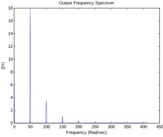
Example 3. Consider a simple nonlinear system described as

3 2

) 1 ( ) 1 ( ) 1 ( 3 . 0 ) 2 ( 5 . 0 ) 1 ( 3 . 0 )

(t = y t− + y t− + u t− +ayt− +byt− y

which can be written in the form (23) with c_1,0(1)=0.3,c_1,0(2)=0.5,c_0,1(1)=0.3,

b c

a

c_2,0(1,1)= , _3,0(1,1,1)= else c_p,q(⋅)=0 , and K=2, M=3. There are only pure output

nonlinearities in this model. Let u(t)=10sin(50t). Consider two cases: (1) c2k,0(.)=0 and

c2k+1,0(.)≠0 , i.e., a=0 and b=-0.005; (2) c2k,0(.)≠0 and c2k+1,0(.)=0, i.e., a=-0.005 and b=0.

0 50 100 150 200 250 300 350 400 450 0

1 2 3 4 5 6 7 8

Output Frequency Spectrum

2|

Y

|

[image:19.595.142.454.109.374.2]

Frequency (Rad/sec)

Figure 1. System output spectrum when a=0 and b=-0.005

0 50 100 150 200 250 300 350 400 450 0

2 4 6 8 10 12 14 16 18

Output Frequency Spectrum

2|

Y

|

Frequency (Rad/sec)

[image:19.595.134.453.413.680.2]