Acoustic modeling using the digital waveguide mesh

This is a repository copy of

Acoustic modeling using the digital waveguide mesh

.

White Rose Research Online URL for this paper:

http://eprints.whiterose.ac.uk/3708/

Article:

Murphy, Damian orcid.org/0000-0002-6676-9459, Kelloniemi, Antti, Mullen, Jack et al. (1

more author) (2007) Acoustic modeling using the digital waveguide mesh. IEEE Signal

Processing Magazine. pp. 55-66. ISSN 1053-5888

https://doi.org/10.1109/MSP.2007.323264

[email protected]

https://eprints.whiterose.ac.uk/

Reuse

Items deposited in White Rose Research Online are protected by copyright, with all rights reserved unless

indicated otherwise. They may be downloaded and/or printed for private study, or other acts as permitted by

national copyright laws. The publisher or other rights holders may allow further reproduction and re-use of

the full text version. This is indicated by the licence information on the White Rose Research Online record

for the item.

Takedown

If you consider content in White Rose Research Online to be in breach of UK law, please notify us by

promoting access to White Rose research papers

White Rose Research Online

Universities of Leeds, Sheffield and York

http://eprints.whiterose.ac.uk/

White Rose Research Online URL for this paper:

http://eprints.whiterose.ac.uk/3708/

Published paper

Murphy, D., Kelloniemi, A., Mullen, J. and Shelley, S. (2007) Acoustic Modeling

Using the Digital Waveguide Mesh , IEEE Signal Processing Magazine, Volume

24 (2), 55 - 66.

©

DIGIT

AL

VISION

T

simulation technique based on the definition of a regular spatial sampling grid for a particular prob-lem domain, which in this specific case is a vibrating object capable of supporting acoustic wave propaga-tion resulting in sound output. It is based on a simple and intu-itive premise—the latter often considered important by the computer musicians who are the primary users of a sound syn-thesis algorithm—yet the emergent behavior is complex, natu-ral, and capable of high-quality sound generation. Hence, the DWM has been applied in many areas of computer music research since it was first introduced by Van Duyne and Smith in 1993 [1]. This article is the first to attempt to consolidate and summarize this work. The interested reader is also directed to [2], where DWM modeling is considered in the more general

context of discrete-time physics-based modeling for sound syn-thesis, and [3], where the DWM is examined within a rigorous theoretical and comparative framework for more established yet related wave scattering numerical simulation techniques.

THE ONE-DIMENSIONAL DIGITAL WAVEGUIDE

The one-dimensional (1-D) digital waveguide is based on a time and space discretization of the d’Alembert solution to the 1-D wave equation. This approach to sound synthesis was first used in the Kelly-Lochbaum model of the human vocal tract for speech synthesis [4] and has parallels with other, more generally applied wave variable scattering modeling paradigms such as the transmission line matrix (TLM) method [5] and wave digital fil-ters (WDFs) [6]. However it was Julius O. Smith III who first proposed the term digital waveguideand used these techniques

Acoustic Modeling

Using the Digital

Waveguide Mesh

[

Recent activities in articulatory vocal tract modeling, room

impulse response synthesis, and reverberation simulation

]

1053-5888/07/$25.00©2007IEEE IEEE SIGNAL PROCESSING MAGAZINE [55] MARCH 2007

initially for artificial reverberation [7] and later for sound syn-thesis [8], [9]. Digital waveguides have remained the most popu-lar and successful physical modeling-based sound synthesis technique to date, due to the realistic, high-quality sounds that can be generated, often in real-time and so therefore also facili-tating effective user interaction. This research has also been made more widely accessible through a range of commercially available physical modeling hardware synthesizers developed by Yamaha in the early 1990s based on digital waveguide tech-niques [10]. The reader is referred to [9] and [11] for a thorough treatment and discussion of this area and a full derivation of some of the equations that are introduced in what follows. Consider the 1-D wave equation for transverse motion with speed con an ideal, infinitely long, vibrating string:

∂2y(t,x) ∂t2 =c

2∂2y(t,x)

∂x2 . (1)

The d’Alembert or traveling wave solution to (1) is defined as:

y(t,x)=y+_(t−x/c)+y−_{(t+x/c), (2)}

where y+ _{and y}− _{are arbitrary twice-differentiable functions}

denoting wave movement to the left and right, respectively. Assuming that y+ _{and y}− _{are bandlimited to half the sampling}

rate of the system allows the discrete time version of (2) to be defined for spatial sampling points mX and sampling interval

nTsuch that X₌cT:

y(nT,mX)=y+_(n−m)+y−_{(n+m). (3)}

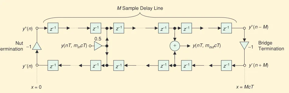
This solution can be implemented in an efficient and straight-forward manner using two parallel digital delay lines to repre-sent the left-going and right-going traveling wave components. Figure 1 shows a digital waveguide implementation of an ideal string, rigidly terminated at either end of the M-sample delay lines, corresponding to the nut and bridge of a typical instru-ment. The system is excited with an appropriate input “loaded’’ into the upper and lower delay lines at position xin=mincT and a physical output is obtained at xout=moutcT by

sum-ming the upper and lower values according to (3), being exact at the sampling points of the system.

THE SCATTERING JUNCTION

The terminations introduced in the 1-D string shown in Figure 1 are a special case of signal scattering. An input signal will propa-gate without loss until it is incident upon a change in system impedance, resulting in transmission and/or reflection of the incident signal. This example leads to the formal definition for a lossless scattering junction, now given without loss of generality in terms of acoustic pressure rather than string displacement. At such a junction, system continuity must be preserved in terms of pressures and volume velocities analogous to Kirchhoff’s Laws for parallel connection of electrical circuit ele-ments. Assuming N connected waveguide elements with the pressure in each defined as piand volume velocities as ui,then for lossless scattering the following must hold:

p1=p2=. . .₌pi=. . .₌pN=pJ, (4)

u1=u2=. . .=ui=. . .=uN=0 (5)

Note that pJis defined as the actual pressure value at the point of connection for these Nwaveguide elements, referred to as the pressure value at scattering junction J. Scattering junctions, together with the 1-D waveguide elements described above, pro-vide the basic building blocks for a digital waveguide physical model of a vibrating system. For instance, six 1-D strings could be coupled together via a scattering junction to simulate the bridge of a guitar, facilitating sympathetic resonances where excitation on one string causes low-amplitude oscillation on one or more of the others due to energy transmitted through the bridge. Similarly, this scattering junction could also allow cou-pling to a filter to simulate the effects of body resonances. Hence, scattering junctions also act as system sampling points where physical variables may be tapped off for coupling with other aspects of the model or with the outside world. Similarly, they can also be used to allow energy to be input to a system. In mod-eling a wind instrument such as a clarinet, the bore can be implemented as a 1-D lossless waveguide coupled with the more

[FIG1]The ideal lossless 1-D digital waveguide string model, which is M_{-samples long and rigidly terminated at either end.}

−1

−1

0.5

x = 0

z−1 _z−1 _z−1

z−1 _z−1

z−1

z−1

z−1

z−1

z−1

x = McT y(nT, moutcT)

y(nT, m_incT)

y+_{(n − M)}

y+_(n)

y−_(n) y−_{(n + M)}

M Sample Delay Line

Bridge Termination Nut

Termination

z−1

z−1

IEEE SIGNAL PROCESSING MAGAZINE [57] MARCH 2007

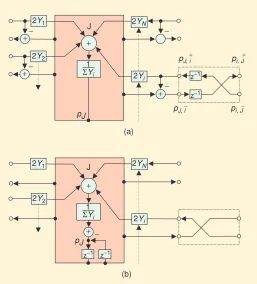
complex, nonlinear breath pressure/reed input function via an appropriate scattering junction implementation [9]. Figure 2(a) shows the functional block diagram for a general lossless scattering junction Jwith Nneighbors, with each connected unit waveguide element having an associated admittance Yi. The impedance of a waveguide is given by Zi=pi/ui and hence the admittance

Yi=1/Zi. The signal p+J,irepresents the incomingsignal to junction Jalong the waveguide from the opposite junc-tion i. Similarly, the signal p−

J,i represents the outgoing signal from junction Jalong the waveguide to the oppo-site junction i. Connecting delay lines together at scatter-ing junctions in a more general sense allows spatial and temporal sampling grids to be defined and gives rise to families of models that are more generally known as digi-tal waveguide networks (DWNs). The Kelly-Lochbaum vocal tract model and the simply terminated 1-D string as shown in Figure 1 are both examples of specific DWNs. A DWN with a more complex arrangement of multiport interconnections can be used to simulate reverberation, as in the first application of digital waveguides [7] and more recently explored in [12]. However a DWN consisting of (typically) unit delay waveguide elements and N-port loss-less scattering junctions conforming to a regularly arranged and spaced grid structure gives rise to a particu-lar family of two- or three-dimensional (2-D or 3-D) struc-tures. These are called digital waveguide meshesand are more directly analogous in construction to the physical objects they are attempting to simulate.

THE DIGITAL WAVEGUIDE MESH

The DWM was first proposed by Van Duyne and Smith [1] as an extension to 1-D digital waveguide sound synthesis appropriate for modeling plates and membranes, potentially leading to full 3-D object modeling. Acoustic wave propagation through a DWM is determined according to the scattering equations and associated mesh topology. For a lossless junction Jaccording to conditions (4) and (5) or directly from Figure 2(a), the sound pressure pJat junction Jfor N connected waveguides can be expressed as:

pJ=

2N_i=1Yi·pJ,_i+

N i=1Yi

. (6)

Noting from (3) that the total sound pressure pJin a waveguide element connected to junction Jcan also be defined as the sum of the traveling waves in this element, or alternatively as the sum of the input and output gives:

pJ=p+J,i+p−J,i. (7)

And finally, as the waveguide elements in a DWM are equivalent to bi-directional unit-delay lines, the input to scattering junc-tion Jat time index n, p+

J,i (n) is equal to the output from neighboring junction iinto the connecting waveguide at the

previous time step, p−

i,J(n−1). Expressing this relationship in the z-domain gives:

P+

J,i=z−1·P−i,J. (8)

Hence, from (6) junction pressure values are calculated accord-ing to input values from immediate neighbors, output values are calculated using (7) and then propagated to neighbors via the bi-directional waveguide elements, becoming inputs at the next iteration according to (8). From (6), (7), and (8) via an appropri-ate linear transformation it is possible to derive an equivalent formulation in terms of junction pressure values only:

pJ=

2N_i=1Yi·pi·z−1

N i=1Yi

−pJ·z−2. (9)

Expression (9) can also be derived directly from a finite differ-ence time domain (FDTD) formulation of the 2-D case of the wave equation in (1). The functional block diagram for the scat-tering junction implementation described by (9), equivalent to Figure 2(a), is shown in Figure 2(b). Digital waveguide models represent signal propagation via two directional wave compo-nents and schemes implemented in this way, according to (6), (7) and (8), are termed W-modelsor W-DWMs[2], [13], [14]. A linear transformation of a W-DWM leads to this alternative implementation as a Kirchhoff variable DWM (K-DWM) [2], [FIG2]Functional block diagrams for the general lossless scattering junction J_with N_{neighbors: (a) the W-model case and (b) the K-model} case. Note that in each example a single connecting waveguide element has been connected to terminal Yi.

(a)

(b) 2Y_N 2Y₁

2Yi

J

2Y2

pJ

z−1 z−1

ΣYi

1

2YN

2Y1

2Yi

Σ1Y_i

+

J

+ +

+

+

+ +

2Y_{2 p}

J, i

−

p_{J, i} pJ

−

−

p_{i, J}

+

pi, J

z−1

z−1

−

−

−

[13], [14], as given in (9), and depending on physical quantities only rather than sampled traveling-wave components. In this form, and under certain conditions, a K-DWM can be computa-tionally equivalent to a FDTD simulation.

Mixed modeling scenarios where K-DWM and W-DWM approaches have been interfaced in 1-D via a KW-pipehave been proposed in [14], [15], leading to the formulation of a 2-D hybrid DWM [13], [16], [17]. The 2-D hybrid mesh combines the computational efficiency of the K-DWM approach in terms of computation time and memory use, with the flexibility of scattering-based boundary termination options for complex geometries through the use of KW-pipes. Typically, KW-hybrid DWMs demonstrate a speed up in processing time of the order of 34% with a 50% decrease in use of main system memory [16]. A K-DWM scattering junction connected to a W-DWM scattering junction via a KW-pipe is shown in Figure 3.

The W-DWM or K-DWM scattering equations can be used to implement a range of topologies/structures. In 2-D the most commonly implemented topologies are the four-port rectilinear and six-port triangular mesh structures shown in Figure 4(a) and (b). A thorough comparison of their relative characteristics, together with those of the three-port hexagonal mesh, is pre-sented in [18]. Two-dimensional DWM models based on the rec-tilinear or triangular topology have been most commonly used for synthesis of percussion instruments such as plates, mem-branes, and gongs [19]–[21], as well as for 2-D reverberation modeling [22]. Three-dimensional topologies as shown in

Figure 4(c)–(f) include the rectilinear [23]; tetrahedral [24], [25]; dodecahedral [also known as cubic close packed (CCP)] [26]; and octahedral structures, and a similar analysis of their characteristics is presented in [27].

Three-dimensional DWM structures are applied to a range of sound synthesis applications. The work of [28] combines a 2-D triangular mesh model of a drum membrane coupled to a 3-D rectilinear model of a drum-shell to give a more complete model of a percussion instrument. DWM models have been applied to simulate 3-D resonant objects [26], [29], [30], sometimes in combination or parallel with other digital waveguide models; for instance, to provide synthesis of complex instrument resonances [31], [32], or to simulate a 3-D acoustic space with multiple 2-D cross-sectional simulations [33]. However, most current research activity in 3-D DWM modeling is in its application to the accurate synthesis of acoustic spaces, and this will be dis-cussed in the Applications section.

An additional subset of K-DWMs has also been subject to much investigation and these are based on an interpolated rectilinear mesh structure in either 2-D [34] or 3-D [35]. Interpolated DWMs demonstrate wave propagation characteristics approaching that of triangular/dodecahedral topologies but without the additional overheads of a denser and more complex topological structure.

DWM LIMITATIONS

There are a number of important factors that impose limitations on DWM models as an optimal solution for all sound synthesis

[FIG3]Functional block diagram for a W-DWM scattering junction Jwith Nneighbors connected to a K-DWM scattering junction K via a KW-pipe connecting waveguide element.

2YN

2Y₁

+

−

J

2Y2

2YM

2Y_j K

2Yi

2YN+1

pJ, i

pJ, 1

p_J

z−1

z−2

2Yi

ΣYi

1

ΣYj

1

p_k

z−1 _z−1 −

−

−

− −

− +

+ +

+

+

+

+ +

+

[FIG4]DWM topologies: (a) four-port 2-D rectilinear; (b) six-port 2-D triangular; (c) six-port 3-D rectilinear; (d) 12-port 3-D dodecahedral (CCP); (e) four-port 3-D tetrahedral; (f) eight-port 3-D octahedral.

IEEE SIGNAL PROCESSING MAGAZINE [59] MARCH 2007

applications. One of the most significant advantages of the 1-D digital waveguide that originally made it a realistic proposition for applications in sound synthesis is the computational efficien-cy of the approach when compared with a brute-force numerical solution to the system wave equation. This is further improved through the ability to commute losses to specific lumped points in the system, significantly reducing the number of calculations required per time-step iteration. Unfortunately, the elegance of this approach is lost when moving to higher dimensions. With a DWM-based system, acoustic wave propagation is determined by signal interaction at the scattering junctions and hence a calcu-lation must take place at every junction for every time-step. Reducing the number of scattering junctions reduces the sam-ple rate of the DWM and hence the effective bandwidth of the system. The advantage gained with the DWM approach, howev-er, is in the structural immediacy of the simulation, allowing objects to be defined based only on physical and geometrical def-initions, and the ability to observe and interact with the system at physically relevant or meaningful points.

A more specific DWM limitation is dispersion error, where the velocity of a propagating wave is dependent upon both its frequency and direction of travel, leading to wave propagation errors and a mistuning of the expected resonant modes. The degree of dispersion error is highly dependent upon mesh topol-ogy and has been investigated in, for example, [3], [18], [24], [27]. In 2-D both the interpolated and triangular DWMs demon-strate dispersion characteristics that are substantially reduced to a function of frequency only. In 3-D, minimization of dispersion can be similarly achieved through the use of interpolated or dodecahedral topologies. Appropriate pre- and postprocessing of results from these mesh structures allows offline frequency warping techniques to be used to correct mis-tuned resonances [34], [35]. Alternatively, frequency warping can be incorporated directly as part of a DWM scattering junction [36], [37]. However, although accurate synthesis of resonant modes is required for the dominant low-frequency properties of a vibrat-ing system, dispersion error is considered less important with increasing frequency as modal density increases, and human perception of such variations becomes less critical.Oversampling a DWM can also offer improvements such that the required bandwidth lies within accepted limits, typically 0.25_×fupdate [1], where fupdate for a DWM of dimension Dand spatial sam-pling distance dis generally given by:

fupdate=

c√D

d , (10)

where cis the speed of sound. Ultimately fupdate dictates the quality of audio signal output from a DWM with large sample rates requiring denser meshes, more computer memory, and hence taking longer to run, limiting even the most efficient large-scale K-DWMs to offline generation only.

DWM BOUNDARY TERMINATION

There exist a number of possibilities for terminating a DWM at a system boundary. In [21] a 10 _×10 node 2-D rectilinear DWM is

terminated with single one-pole all-pass filters, which may be interpreted as a 1-D termination connected to an ideal spring, allowing modal frequencies in the DWM to be re-tuned or cor-rected appropriately. For curved boundaries, where the perime-ter of the structure being modeled is not normal/parallel to the axes of the mesh, noninteger length waveguide elements called

rimguidescan be used [20] and have been demonstrated as appropriate for accurate low-frequency modeling of circular membranes using a 2-D triangular mesh.

A commonly applied solution is to passively terminate a DWM using a simple 1-D connection that implements a change in admittance such that there is no signal return from the con-nected boundary over a finite time duration. Hence, the associ-ated input value for such a connection in Figure 2, or using (6) or (9), is set to zero. This termination acts to reflect an incident signal according to the change in admittance of the connected waveguide elements. In the simplest case, for a one-port bound-ary-node pBconnected to a single N-port scattering junction p1 with a change in waveguide admittance from Yto YB, a reflec-tion coefficient ₋1_≤r_≤1 is determined such that:

r=Y−YB

Y+YB

(11)

and pB can therefore be calculated as a function of the sound pressure of the incident traveling wave variable from p1:

pB=(1+r)·pB,1+. (12)

In the equivalent K-DWM case, a passive termination is equiva-lently implemented as a feedback loop between waveguide ele-ment terminals in Figure 2 with unit delay as derived in [13], [38] and given by

pB=(1+r)p1·z−1−r·pB·z−2. (13)

Note that r₌1 or r_{= −}1 gives total reflection and r₌0 approximates anechoic conditions. Full derivations of boundary conditions for the general N-port boundary termination for K-, W-, and KW-hybrid cases is offered in [16] and a similar bound-ary implementation for a triangular DWM using multiport reflection factors is presented in [29].

APPLICATIONS OF THE DWM

The digital waveguide mesh in 2-D and 3-D has been applied to a diverse range of applications where simulation of acoustic wave propagation within an enclosed system is required. What follows is a summary of recent results and research in this area, namely for vocal tract synthesis, object modeling, synthesis of room impulse responses, and how this method can be extended to abstract higher dimensions.

2-D VOCAL TRACT MODELING FOR SPEECH SYNTHESIS

section implemented as a 1-D digital waveguide element. A number of developments on this basic model include nasal tract, lip radiation, and wall losses to synthesize the singing voice [39] and the use of fractional waveguides to make lengthwise changes to tract shape [40],

[41]. Standard waveguide ele-ments have also been substitut-ed for conical equivalents using scattering methods derived from the spherical wave equa-tion. This increases model accuracy, giving higher-order area function approximation, but adds to the computational load and introduces possible

stability problems [40], [42]. More recent work has explored the possibility of replacing the basic 1-D digital waveguide imple-mentation with a 2-D DWM model that simulates the variation in cross-sectional area along the vocal tract directly through an appropriately shaped mesh geometry [43]. Formant patterns produced using the 2-D DWM implementation are equivalent to those produced by a very high-resolution 1-D digital waveguide acoustic tube-based simulation. The 2-D model also offers simu-lation of cross-tract modes due to the additional dimension of freedom for acoustic oscillation and propagation and approxi-mately linear control over formant bandwidths via the addition-al reflection parameter at the side waddition-alls of the vocaddition-al tract. Hence, the 2-D DWM vocal tract offers improvements similar to other developments based on enhanced-order acoustic tube area function approximation, together with additional model flexibil-ity such as the abilflexibil-ity to simulate a split in the air channel used in the creation of sounds such as /l/.

The disadvantages of this proposed voice synthesis mecha-nism rest in its inability to simulate smooth, continuous dynamic changes to the tract area functions to facilitate artic-ulated voice synthesis, and the high mesh sample rate fupdate required to ensure accurate tracking and mapping of vocal tract shape resulting in an implementation that can only work offline. Both of these problems have been analyzed and a solu-tion proposed in a new implementasolu-tion of the 2-D DWM [44]. In this new method, rather than mapping acoustic tube area function directly to the 2-D DWM geometry, a constant-width 2-D rectangular DWM, 17.5 cm long with fupdate=44.1 kHz is used. The waveguide element impedance across the width of this rectangular geometry is then varied according to the

area function information. A minimum impedance channel

Zminis defined as the lowest value across the range of vowels to be simulated, corresponding directly to the largest cross-sectional area Amax, and from this a maximum tract width opening can be defined. An

impedance mapis constructed for a particular vowel tract shape such that each area func-tion value A(x) along the length of the tract walls corre-sponds to a maximum imped-ance value Zx. An impedance curve varying from Zx to Zmin and back to Zx at the opposite wall is then defined across the tract according to a raised cosine function, with the mini-mum impedance channel equidistant between the tract walls.

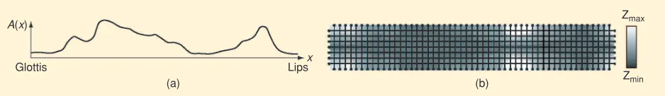
Figure 5(a) shows the cross-sectional area function informa-tion A(x)taken from MRI scans [45] as it varies along the length of the vocal tract from glottis to lips. Figure 5(b) is the corre-sponding impedance map imposed across and along the under-lying rectangular 2-D DWM based on a four-port rectilinear topology. Areas of higher impedance are represented by a lighter shading, and the minimum impedance channel can be observed as the darker area along the center of the map. Figure 6(a) shows the resulting formant pattern for this vocal tract shape, when excited by a noise source at the glottis and measured at the lip end. The dotted lines have been generated from a high-resolution 1-D waveguide model, using the same area functions for comparison purposes, and measured average formant values are also shown.

Software developed to test the real-time dynamic behavior of this 2-D DWM vocal tract model is available for download and use at [47], and initial results based on this system were first pre-sented in [44]. This application also facilitates real-time dynamic articulation. An example is presented in Figure 6(b) demonstrat-ing a smooth linear interpolation between area function data for the /a/ (“bard’’) and /e/ “bed’’) vowels under noise source excita-tion to highlight the resulting change in formant patterns.

Figure 6 shows that this new 2-D dynamically varying DWM demonstrates results in terms of simulated formant frequencies that are in good agreement with both a high-resolution 1-D model and real-world values. Figure 6(a) seems to indicate that the 2-D model is closer to real-world formant values than the high-resolution 1-D case, although this accuracy actually varies

[FIG5]Forming the impedance mapped /u/ vowel DWM: (a) cross-sectional area function; (b) rectilinear mesh with raised cosine impedance map.

A(x)

x

(a)

Glottis Lips

(b)

Zmax

Z_min

DIGITAL WAVEGUIDES HAVE

REMAINED THE MOST POPULAR

AND SUCCESSFUL PHYSICAL

MODELING-BASED SOUND SYNTHESIS

TECHNIQUE TO DATE, DUE TO THE

REALISTIC, HIGH-QUALITY SOUNDS

IEEE SIGNAL PROCESSING MAGAZINE [61] MARCH 2007

with target vowel/tract-shape and the real-world values used. In general, the two modeling methods are in good agreement with one another. Also, Figure 6(b) demonstrates a smooth transition between vocal tract shapes without any discontinuity for the 1-D and 2-D cases, being of particular importance in the latter exam-ple. Hence, from these generally comparable results the 2-D dynamically varying DWM can be seen to offer an alternative to current 1-D dynamic vocal tract models, while also offering additional advantages over these 1-D implementations as dis-cussed above and presented in [43] for static simulations of the vocal tract. The reader is invited to test the software presented in [47] and compare the audio output from both 1-D and 2-D models under LF glottal source excitation. Informal perceptual testing has demonstrated that users consider the 2-D example to be more “natural-sounding’’ than the similar 1-D case.

This work is the first demonstration of a dynamically varying DWM model, in this case operating in real-time. Most prior DWM work has been based on a static representation of the acoustic system under study, partly due to the computational resources required for real-time implementation and user inter-action, and partly due to possible discontinuities in the output from the resulting model. Hence, this work potentially opens new areas of research and application areas for DWM modeling, possibly moving to direct user-input and feedback that has cur-rently only been possible in 1-D digital waveguide synthesis. Further work in this area will concentrate on developing appro-priate tract wall boundary filters and facilitate lengthwise shape changes for modeling lip protrusion required for accurate syn-thesis of the /u/ vowel. This work also demonstrates the poten-tial of moving toward a full 3-D DWM model using 3-D MRI scans of the vocal tract shape incorporating complex-shape cross-sectional area data.

2-D OBJECT MODELING

The DWM is often used to synthesize the acoustic properties of a 2-D or 3-D resonant body as these objects are a fundamental

component of most musical instruments, serving to both ampli-fy and modiampli-fy the characteristics of a source excitation. Given that the resonating aspects of most instrument bodies are rela-tively small implies that a high-resolution DWM implementa-tion is feasible—in real-time in the case of the vocal tract model above—with modern computing facilities. Consider the classic example of a 2-D ideal stretched circular membrane. The reso-nant frequencies fmncan be defined according to the nature of their nodal regionswhere mrepresents the number of nodal lines positioned along the diameterof the membrane and n rep-resents the number of circular nodal lines, including the bound-ary. The fundamental frequency of an ideal membrane f01can be calculated according to its physical properties (for example, as presented in [19]). Subsequent modes are fixed relative to f01. Figure 7(a) shows the nodal regions of an ideal stretched cir-cular membrane with diameter 0.5 m, implemented using a highly oversampled 2-D triangular DWM, with fupdate=192 kHz, resulting in a spatial sampling distance of 0.00253 m and a total of 35,742 junctions. The membrane is excited near the boundary with a lowpass-filtered impulse and an output is obtained at a junction near the opposite boundary. To model an ideal membrane with clamped edges, the reflection coefficients r

at the boundary of the mesh are set to ₋1. The modes (0,2), (1,1), (2,1), and (3,1), are shown, with associated frequencies given relative to f01. Figure 7(b) plots the spectrum of the out-put against the theoretical predicted frequencies for the funda-mental and first nine modes.

Note that from Figure 7(b) there is an exact correlation between the predicted modal frequencies and those obtained via simulation, and this is due to the high mesh sample rate used, minimizing dispersion error effects for the bandwidth studied, and ensuring a smooth mesh fit to the circular boundary of the membrane without using rimguides.

An exciting possibility with physical modeling synthesis is that, with clear defined rules governing system behavior, it becomes relatively straightforward to extend these rules to

[FIG6]Formant patterns from the impedance-mapped DWM under noise excitation: (a) /u/ vowel compared with a high resolution 1-D model and average measured values; (b) /a/ to /e/ diphthong compared with same 1-D model.

5

4

3

2

1

0

0 0.25 0.5

/a/ /e/

f/kHz

t/s

1-D Formants

(b)

−20

−40

−60

−80

−100

dB

0 1 2 3 4 5

kHz (a)

f1 f2 f3 f4

situations that could not exist, or are difficult to control, in the real world. Figure 8 presents one such example as an extension of the 2-D circular membrane and shows the two lowest modes of resonance from a DWM membrane simulation of a tri-foil radiation symbol with diameter and fupdateas before, this time resulting in a model consisting of 25,549 junctions. Sound examples for these simple 2-D objects are available at [48]. In isolation the sounds produced from such basic 2-D membranes, although percussive in nature, are somewhat uninspiring and require a more complete model for accurate and interesting object synthesis and, hence, these examples should be consid-ered as a starting point only. Further research in improved modeling of resonant objects has considered DWNs for more complex theoretical multidimensional systems [3], specific

aspects such as coupling a 2-D membrane to a 3-D resonator [28], improved nonlinear excitation [49], and using simple DWM resonators to model the high-frequency characteristics of complex instrument bodies [31]. Also of note is the Sounding Object Project that has explored physical modeling, including 2-D and 3-D DWMs of resonating objects, with a view to match-ing the perception of synthesized sounds to the modeled objects that created them [26], [29], [50].

SYNTHESIS OF ROOM IMPULSE RESPONSES

The first application of DWMs in the field of room acoustics sim-ulation was by Savioja et al. in 1994 [23]. Fundamentally, syn-thesizing the characteristics of a bounded space using a DWM is exactly the same as synthesizing the sound of a vibrating

[FIG8]2-D triangular DWM model of a physically impossible system—a trifoil radiation symbol membrane with a diameter of 0.5 m: (a) animation captures from the resulting simulation demonstrating modal resonances; (b) output spectrum.

(a)

10

−10

−20

−30

−40

−50

−60

−70

−80 0

2,600 2,800 3,000 3,200 3,400 3,600 3,800 4,000 Frequency (Hz)

(b)

Po

w

er (dB)

[FIG7]2-D triangular DWM model of a membrane with a diameter of 0.5 m: (a) animation captures from the resulting simulation demonstrating resonance at modes (0,2), (1,1), (2,1), and (3,1); (b) actual output spectrum compared with predicted modal frequencies.

−10

−20

−30

−40

−50

−60

−70

−80

0 500 1,000 1,500 2,000

Frequency (Hz)

(b) f01

f11

f21

f02

f31 f12 f11

f22

f₀₃

f51

Po

w

er (dB)

(a)

f₀₂ = 2.30 f11 =1.59

f₂₁ = 2.14

IEEE SIGNAL PROCESSING MAGAZINE [63] MARCH 2007

physical object. However, in the latter example, sound output is generated directly from the modeled object by reading sample values at a scattering junction, whereas with room acoustics modeling it is a room impulse response (RIR) that is synthesized rather than the actual sound source. The RIR is generally of lit-tle interest in terms of its direct audio quality; however, when convolved with an arbitrary anechoic audio input the result is to perceive the audio source as if placed within the modeled space. Also, the relative size of the DWMs used as 3-D acoustic spaces are many times larger than, for example, the 2-D vocal tract pre-sented above, and hence take considerably longer to execute, implying offline RIR synthesis only.

It has been shown that DWMs offer accurate RIR synthesis at low frequencies [51] and demonstrate natural wave phenomena such as interference and diffraction [52], with high-frequency accuracy being limited by fupdateand the dispersion error of the selected topology. This contrasts with other RIR synthesis meth-ods based on geometric acoustic techniques [53] that are typi-cally valid for high frequencies only. Other research has explored how 3-D spaces, or their reverberant characteristics, might be simulated using 2-D models, significantly reducing computational resources [22], [33]. However, the accurate simu-lation of DWM boundaries is still a key research area with a view to how the physical properties of real materials might be mod-eled. This has included how 1-D boundary termination might be optimized for anechoic conditions [54] [55], leading to a new spatially averaged approach for the 0≤r≤1 case [56].

Optimized absorption/reflection across a wide range of angles of incidence for −1≤r≤1 has been facilitated using the

admit-tance boundarymethod [57], where a DWM is terminated with additional layers of boundary-nodes behind the actual boundary location, in turn terminated using an optimal anechoic solution. For accurate simulation of real acoustic boundaries, frequen-cy-dependent reflection/absorption must be implemented. In [58], a boundary-node is replaced with a boundary filter defined to optimally match given frequency-dependent material reflec-tion coefficients and implemented using a first-order infinite impulse response filter for a 2-D rectilinear K-DWM. This results in a good approximation to the target response but is subject to the directional-dependent characteristics of the mesh topology, being less accurate for certain angles of incidence.

The other important characteristic of a real-world acoustic boundary is whether a reflection is specular, where the angle of

reflection is equal to the angle of incidence, or diffusesuch that the incident energy is redistributed over a range of angles. Previous diffuse boundary implementations for a DWM are effec-tive but limited, either in terms of accuracy [20], or by sacrific-ing user control for an optimal solution [59]. A new technique based on [20] simulates accurate diffusion with a high degree of control and consistency by rotating incoming junction signals via a circulant matrix at a diffusing layerof standard N-port W-DWM air-nodes adjacent to the boundary [60]. The model is lossless and allows other boundary conditions, such as frequen-cy-dependent absorption, to be easily incorporated.

Much of this recent application-focused research has been incorporated as part of the RoomWeaver DWM-based room acoustics research tool first presented in [17] and shown in Figure 9. The purpose of the system is to allow the user to intu-itively set up enclosed space geometry, boundary surface, and source/receiver parameters required to generate an RIR by means of a simple scripting language and graphical user inter-face. High-quality reverberation and auralization for a wide range of spaces/applications are possible using high-resolution 2-D triangular and 3-D mesh topologies both based on a KW-hybrid implementation. A range of RIRs synthesized according to varied initial conditions and associated audio examples are available for download [48]. For complete synthesis of a sound event it would be desirable to incorporate a 3-D dynamically variable instrument model within a larger 3-D DWM of a per-formance space, requiring appropriate interfacing across DWM types according to the space and instrument models used. Although nontrivial, this has been considered in the case of a drum model using a 2-D triangular DWM membrane with a 3-D rectilinear shell [28] and in the more general case [3]. However, such complete synthesis could only be offered via the offline RIR generation/real-time convolution processing paradigm due to the computational expense of full 3-D space modeling. Such examples are presented in [48] for a 2-D DWM vocal tract processed with DWM-synthesized RIRs.

THE HYPER-DIMENSIONAL DIGITAL WAVEGUIDE MESH

From (6) it is clear that dimensionality is not inherent in the scattering equations. For example, the four-port lossless scat-tering junction is the main algorithmic building block of both the 2-D rectilinear and 3-D tetrahedral mesh. The spatial arrangement of the surrounding scattering junctions—the

mesh topology—is the determining factor and it is therefore possible to extend the scattering junction concept beyond three spatial dimensions to hyper-dimensional DWMs[23], [61] that have been shown as appropriate for simulating artifi-cial reverberation [62].

At low frequencies, the acoustic characteristics of a room can be modeled with sufficient accuracy by approximating the main dimensions of a basic cuboid model and simulating the corresponding resonant modes. In real rooms there are typically additional architectural features that lead to fre-quency-dependent irregularity in these predicted trajectory lengths. Hence, at higher frequencies, a typical RIR will demonstrate a large number of densely and irregularly dis-tributed modal peaks that are not determined by the basic geometry of the space alone. However, for high-quality artifi-cial reverberation not all of these modes need to be simulated directly, with approximately 1,500 modes distributed evenly or along a logarithmic scale between 80 Hz and 10 kHz being sufficient for diffuse and natural sounding artificial reverber-ation [63]. In a DWM, the number of primary resonant modes is equal to the number of dimensions, with higher dimen-sions leading to a more irregular arrangement of modal peaks. It is possible to extend these equations describing the resultant wave propagation to the hyper-dimensional case, where for each mesh dimension xi the primary mode has a frequency corresponding to (c/2Li) with Li defined as the trajectory length. In an N-dimensional space, standing waves occur at the following frequencies:

fn1n2n3...nN= c

2

_N

i=1 _n

i

Li 2

, (14)

where ni is the integer index of the current mode for each dimension and cis the speed of sound. Furthermore, at a

specif-ic modal frequency, the sound pressure value at a point (x1, x2,

x3, . . . ,xN)inside such space is determined by:

pn1n2n3...nN(x1,x2,x3, . . . ,xn)=A N

i=1 cos

_n ixi

Li

, (15)

where Ais an arbitrary amplitude coefficient.

Examples of modal distributions calculated using (15) are shown in Figure 10(a). Note that the additional advantage of a hyper-dimensional DWM reverb is the resultant high-densi-ty distribution of high-frequency modes while simultaneous-ly avoiding potentialsimultaneous-ly problematic (in terms of perceived sound quality) low-frequency resonances. This is due to the trajectories being kept shorter compared to a similar model with the same number of junctions but lower dimensionality and is demonstrated in Figure 10(b) comparing 2-D and four-dimensional DWMs. Hence, hyper-four-dimensional DWM reverb satisfies the requirement for a densely distributed high fre-quency modal response while giving the freedom for the more precise and sparsely arranged low-frequency modes to be modeled with any other appropriate technique without frequency overlap. Further work for a more natural reverber-ant effect requires the implementation of frequency-depend-ent losses to simulate air and boundary absorption as used in RIR synthesis with standard 2-D and 3-D DWM models.

CONCLUSIONS

The digital waveguide mesh has been an active area of music acoustics research for over ten years. Although founded in 1-D digital waveguide modeling, the principles on which it is based are not new to researchers grounded in numerical simulation, FDTD methods, electromagnetic simulation, etc. This article has attempted to provide a con-siderable review of how the DWM has been applied to acoustic modeling and sound synthesis problems, including

[FIG10]Frequency response information for 2,310 node DWMs of varying dimension: (a) theoretical modal distribution varying with increasing dimensionality; (b) frequency response of a 2-D and 4-D DWM.

1,000

800

600

400

200

0

0 0.05 0.1

Relative Frequency (1/fs)

(a) (b)

Relative Frequency (1/fs) 0.15 0.2 0.25

Number of Modes

1-D 2-D 3-D 4-D 5-D

50

Magnitude (dB)

0

0.25 0.2

0.15 0.1

0.05 0

−50

50

Magnitude (dB)

0

0.25 0.2

0.15 0.1

0.05 0

−50

2-D

IEEE SIGNAL PROCESSING MAGAZINE [65] MARCH 2007

new 2-D object synthesis and an overview of recent research activities in articulatory vocal tract modeling, RIR synthe-sis, and reverberation simulation. The extensive, although not by any means exhaustive, list of references indicates that though the DWM may have parallels in other disci-plines, it still offers something new in the field of acoustic simulation and sound synthesis. Perhaps one reason for the continued interest in this area is the natural and intuitive complex emergent behavior that results from such simple, locally defined scattering equations. However, despite this perceived simplicity, it is also clear that there are still many nontrivial problems to be solved. There are few current examples of useful and playable virtual instruments using DWM based sound synthesis (although a virtual drum in the London Science Museum that can be played in real-time and is a realization of the work presented in [28] is a notable exception), and this is mainly due to the computa-tional resources required for such a real-time model. Nonreal-time operation is not a problem when simulating static, linear time-invariant systems such as a representa-tion of an acoustic space, and hence most recent DWM work has focused in this area. The real-time convolution of an audio input signal with the impulse response generated from such a model is trivial to implement on a modern computing platform and is now a commonly used sound processing operation. Offline, only DWM-based virtual instruments for sound synthesis prohibit user interaction and severely limit playability. However, some of the recent developments presented in this article, particularly those relating to dynamic, real-time vocal tract simulation, are beginning to make significant inroads in this area and will hopefully lead to new DWM implementations that can be applied more generally—and more successfully—to the diverse range of possible sound synthesis applications.

ACKNOWLEDGMENT

This work is supported in part by the U.K. Engineering and Physical Sciences Research Council (EPSRC), grant number GR/S01481/01, and in part by the Swedish Foundation for International Cooperation in Research and Higher Education (STINT), contract IG2002-2049. Antti Kelloniemi has received funding from the Academy of Finland (project 201050) and the Nokia Foundation.

AUTHORS

Damian T. Murphy([email protected]) received the B.Sc. (Hons) in mathematics in 1993; the M.Sc. in music technolo-gy in 1995; and the D.Phil. in music technolotechnolo-gy in 2000, all from the University of York, York, U.K. He is currently a lec-turer in the Department of Electronics, University of York, and a visiting lecturer in the Department of Speech, Music and Hearing, KTH, Stockholm, Sweden. His research inter-ests include physical modeling, spatial sound, and applica-tions of the digital waveguide mesh. Dr Murphy is a member of the Audio Engineering Society.

Antti Kelloniemi([email protected]) received his M.Sc. from the University of Helsinki, Finland, in 2003. He is current-ly finalizing his doctoral thesis, “Room acoustics modeling with the digital waveguide mesh—Boundary structures and approxi-mation methods,’’ at the Helsinki University of Technology. He has recently been appointed as the technology manager for loudspeaker manufacturer Panphonics Oy, where his research concentrates mainly on electrostatic loudspeakers and active noise control. His interests include the modeling and design of acoustics and audio electronics.

Jack Mullen ([email protected]) received the M.Eng. in electronic engineering with music technology from the University of York, York, U.K., in 2002. His final year M.Eng. project involved research into digital waveguide mesh boundary implementations for room acoustics model-ing. He has recently been awarded a Ph.D. degree from the University of York in 2006 for his thesis on multidimensional waveguide vocal-tract modeling. His research interests include speech and acoustical modeling.

Simon Shelley([email protected]) received the M.Eng. in electronic engineering with music technology sys-tems from the University of York, U.K., in 2003. He is now work-ing toward a Ph.D. on the accurate modelwork-ing of acoustic boundaries in the digital waveguide mesh, which is to be com-pleted in 2007. Research interests include acoustic modeling, sound spatialization, and human–computer interaction for musical applications.

REFERENCES

[1] S.A. Van Duyne and J.O. Smith, “Physical modeling with the 2-D Digital waveguide mesh,’’ in Proc. Int. Computer Music Conf., Tokyo, Japan, 1993, pp. 40–47.

[2] V. Välimäki, J. Pakarinen, C Erkut, and M. Karjalainen, “Discrete time modeling of music instruments,’’ Rep. Prog. Phys., vol. 69, pp. 1–78, Jan. 2006. [Online] Available: http://www.iop.org/EJ/abstract/0034-4885/69/1/R01/

[3] S. Bilbao, Wave and Scattering Methods for Numerical Simulation. Chichester, UK: Wiley, 2004.

[4] J.L. Kelly and C.C. Lochbaum, “Speech synthesis,’’ in Proc. Fourth Int. Congr. Acoustics, Copenhagen, Denmark, Sept. 1962, pp. 1–4.

[5] P.B. Johns and R.L. Buerle, “Numerical solution of 2-dimensional scattering problems using a transmission line matrix,’’ Proc. IEE, vol. 118, pp. 1203–1208, Sept. 1971.

[6] A. Fettweis, “Digital filters related to classical structures,’’ AEU: Archive für Elektronik und” Ubertragungstechnik,vol. 25, pp. 78–89, Feb. 1971.

[7] J.O. Smith, “A new approach to digital reverberation using closed waveguide networks,’’ in Proc. Int. Computer Music Conf., Vancouver, Canada, 1985, pp. 47–53.

[8] J.O. Smith, “Music applications of digital waveguides,’’ CCRMA, Stanford Univ., Stanford, CA, Tech. Rep. STAN-M-39, 1987.

[9] J.O. Smith, “Physical modeling using digital waveguides,’’Computer Music J., vol. 16, no. 4, pp. 74–87, 1992.

[10] Stanford University News Service, “Music synthesis approaches sound quality of real instruments,’’ Stanford University News Release, July 1994. [Online] Available: http://www.stanford.edu/dept/news/pr/94/940607Arc4222.html

[11] J.O. Smith, “Principles of digital waveguide models of musical instruments,’’ in Applications of Digital Signal Processing to Audio and Acoustics, M. Kahrs and K. Brandenburg, Eds. Boston, MA: Kluwer, pp. 417–466, 1998.

[12] M. Karjalainen, P. Huang, and J.O. Smith, “Waveguide networks for room response modeling and synthesis,’’ in Proc. 118th AES Conv., Barcelona, Spain, preprint 6394, May 2005.

[14] C. Erkut and M. Karjalainen, “Finite difference method vs. digital waveguide method in string instrument modeling and synthesis,’’ in Proc. ISMA 2003, Mexico City, Dec. 2002.

[15] A. Kelloniemi, “Frequency dependent boundary conditions for the 3-D digital waveguide mesh,’’ in Proc. 9th Int. Conf. Digital Audio Effects (DAFX06), Montréal, Canada, Sept. 2006, pp. 161-164. [Online]. Available: http:www.dafx.ca/proceedings/papers/p_161.pdf

[16] D.T. Murphy and M.J. Beeson, “The KW-boundary hybrid digital waveguide mesh for room acoustics applications,’’ IEEE Trans. Speech Audio Processing, to be published.

[17] M.J. Beeson and D.T. Murphy, “RoomWeaver: A digital waveguide mesh based room acoustics research tool,’’ in Proc. 7th Int. Conf. Digital Audio Effects (DAFX04), Naples, Italy, Oct. 2004, pp. 268–273. [Online]. Available: http://dafx04.na.infn.it/WebProc/Proc/P_268.pdf

[18] F. Fontana and D. Rocchesso, “Signal-theoretic characterization of waveguide mesh geometries for models of two-dimensional wave propagation in elastic media,’’ IEEE Trans. Speech Audio Processing, vol. 9, no. 2, pp. 152–161, Feb. 2001.

[19] F. Fontana and D. Rocchesso, “A new formulation of the 2-D waveguide mesh for percussion instruments,’’ in Proc. XI Colloq. Musical Informatics, Bologna, Italy, Nov. pp. 27–30, 1995.

[20] J. Laird, P. Masri, and N. Canagarajah, “Modeling diffusion at the boundary of a digital waveguide mesh,’’ in Proc. Int. Computer Music Conf., Beijing, China,, Oct. 1999, pp. 492–495.

[21] S.A. Van Duyne and J.O. Smith, “A simplified approach to modeling dispersion caused by stiffness in strings and plates,’’ in Proc. Int. Computer Music Conf., Aarhus, Denmark, 1994, pp. 407–410.

[22] D.T. Murphy and D.M. Howard, “2-D digital waveguide mesh topologies in room acoustics modeling,’’ in Proc. 3rd Int. Conf. Digital Audio Effects (DAFX00), Verona, Italy, Dec. 2000, pp. 211–216 [Online]. Available: http://profs.sci.univr.it/∼

dafx/DAFx-final-papers.html

[23] L. Savioja, T.J. Rinne, and T. Takala, “Simulation of room acoustics with a 3-D finite difference mesh,’’ in Proc. Int. Computer Music Conf., Aarhus, Denmark, 1994, pp. 463–466.

[24] S.A. Van Duyne and J.O. Smith III, “The 3-D tetrahedral digital waveguide mesh with musical applications,’’ in Proc. Int. Computer Music Conf., Hong Kong, 1996, pp. 9–16.

[25] S.J. Miklavcic and J. Ericsson, “Practical implementation of the 3D tetrahedral TLM method and visualization of room acoustics,’’ in Proc. 7th Int. Conf. Digital Audio Effects (DAFX-04), Naples, Italy, Oct. 2004, pp. 262–267. [Online]. Available: http://dafx04.na.infn.it/WebProc/Proc/P_262.pdf

[26] F. Fontana, D. Rocchesso, and E. Apollonio, “Using the waveguide mesh in modeling 3-D resonators,’’ in Proc. 3rd Int. Conf. Digital Audio Effects (DAFX-00), Verona, Italy, Dec. 2000, pp. 229–232 [Online]. Available: http://profs.sci.univr.it/

∼dafx/DAFx-final-papers.html

[27] G.R. Campos and D.M. Howard, “On the computational efficiency of different waveguide mesh topologies for room acoustic simulation,’’ IEEE Trans. Speech Audio Processing, vol. 13, no. 5, pp. 1063–1072, Sept. 2005.

[28] M.L. Aird, J. Laird, and J. Ffitch, “Modeling a drum by interfacing 2-D and 3-D waveguide meshes,’’ in Proc. Int. Computer Music Conf., Berlin, Germany, Aug. 2000, pp. 82–85.

[29] F. Fontana, “Physics-based models for the acoustic representation of space in virtual environments,’’ Ph.D. dissertation, Dept. Computer Science, Univ. of Verona, Italy, Apr. 2003. [Online]. Available: http://profs.sci.univr.it/∼

fontana/paper/20.pdf

[30] D. Rossiter, A. Horner, and G. Baciu, “Visualization and manipulation of 3D digital waveguide structures,’’ in Proc. Int. Computer Music Conf., Beijing, China, 1999, pp. 43–46.

[31] P. Huang, S. Serafin, and J.O. Smith, “A 3-D waveguide mesh model of high-frequency violin body resonances,’’ in Proc. Int. Computer Music Conf., Berlin, Germany, Aug. 2000, pp. 86–89.

[32] S. Serafin, P. Huang, and J.O. Smith, “The banded digital waveguide mesh,’’ in Proc. MOSART Workshop Current Research Directions Computer Music, Barcelona, Spain, Nov. 2001. [Online]. Available: http://www.imi.aau.dk/∼sts/

publications/mosart.pdf

[33] A. Kelloniemi, V. Välimäki, and L. Savioja, “Simulation of room acoustics using 2-D digital waveguide meshes,’’ in Proc. IEEE Int. Conf. Acoustics, Speech, and Signal Processing (ICASSP), Toulouse, France, May 2006, pp. 313-316.

[34] L. Savioja and V. Välimäki, “Reducing the dispersion error in the digital wave-guide mesh using interpolation and frequency warping techniques,’’ IEEE Trans. Speech Audio Processing, vol. 8, no. 2, pp. 184–194, Mar. 2000.

[35] L. Savioja and V. Välimäki, “Interpolated rectangular 3-D digital waveguide mesh algorithms with frequency warping,’’ IEEE Trans. Speech Audio Processing, vol. 11, no. 6, pp. 783–789, Nov. 2003.

[36] F. Fontana and D. Rocchesso, “Online correction of dispersion in 2D wave-guide meshes,’’ in Proc. Int. Computer Music Conf., Berlin, Germany, Aug. 2000, pp. 78–81.

[37] F. Fontana, “Computation of linear filter networks containing delay-free loops, with an application to the waveguide mesh,’’ IEEE Trans. Speech Audio Processing, vol. 11, no. 6, pp. 7743–782, Nov. 2003.

[38] L. Savioja, T. Rinne, and T. Takala, “Simulation of room acoustics with a 3-D finite difference mesh,’’ in Proc. Int. Computer Music Conf., Aarhus, Denmark, Sept. 1994, pp. 463–466.

[39] P.R. Cook, “Identification of control parameters in an articulatory vocal tract model with applications to the synthesis of singing,’’ Ph.D. dissertation, Stanford Univ., Stanford, CA, 1990.

[40] V. Välimäki and M. Karjalainen, “Improving the Kelly-Lochbaum vocal tract model using conical tube sections and fractional delay filtering techniques,’’ in Proc. Int. Conf. Spoken Language Processing (ICSLP), Yokohama, Japan, 1994, pp. 615–618.

[41] S. Mathur and B.H. Story, “Vocal tract modeling: Implementation of continu-ous length variations in a half-sample delay Kelly-Lochbaum model,’’ in Proc. IEEE Intl. Symp. Signal Processing and Information Technology, Darmstadt, Germany, 2003, pp. 753-756.

[42] H.W. Strube, “Are conical segments useful for vocal-tract simulation?’’ J. Acoust. Soc. Amer., vol. 114, no. 6, pp. 3028–3031, 2003.

[43] J. Mullen, D.M. Howard, and D.T. Murphy, “Waveguide physical modeling of vocal tract acoustics: Flexible formant bandwidth control from increased model dimension-ality,’’ IEEE Trans. Speech Audio Processing, vol. 14, no. 3, pp. 964–971, May 2006.

[44] J. Mullen, D.M. Howard, and D.T. Murphy, “Real-time dynamic articulations in the 2D waveguide mesh vocal tract model,’’ IEEE Trans. Speech Audio Processing, submitted for publication, 2006.

[45] B.H. Story, I.R. Titze, and E.A. Hoffman, “Vocal tract area functions from mag-netic resonance imaging,’’ J. Acoust. Soc. Amer., vol. 100, no. 1, pp. 537–554, 1996.

[46] D.G. Childers, Speech Processing and Synthesis Toolboxes. New York: Wiley, 2000.

[47] J. Mullen, D.T. Murphy, and D.M. Howard, “Physical modeling of the vocal tract with the 2-D digital waveguide mesh,’’ [Online]. Available: http://www-users.york.ac.uk/∼_{dtm3/vocaltract}

[48] S. Shelley, “Acoustic modeling—The digital waveguide mesh,’’ [Online]. Available: http://www-users.york.ac.uk/∼dtm3/vocaltract.html

[49] S.A. Van Duyne, J.R. Pierce, and J.O. Smith, “Traveling wave implementation of a lossless mode-coupling filter and the wave digital hammer,’’ in Proc. Int. Computer Music Conf., Aarhus, Denmark, 1994, pp. 411–418.

[50] D. Rocchesso and F. Fontana, Eds., The Sounding Object. Florence, Italy: Mondo Estremo, 2003.

[51] L. Savioja, J. Backman, A. Järvinen, and T. Takala, “Waveguide mesh method for low-frequency simulation of room acoustics,’’in Proc. Int. Congr. Acoustics, Trondheim, Norway, vol. 2, pp. 637–641, June 1995.

[52] D.T. Murphy and M.J. Beeson, “Modeling spatial sound occlusion & diffraction effects with the digital waveguide mesh,’’ in Proc. Audio Eng. Soc. 24th Int. Conf., Banff, Canada, June 2003, pp. 207–216.

[53] U. Stephenson, “Comparison of the image source method & the particle simu-lation method,’’ Appl. Acoust., vol. 29, no. 1, pp. 35–72, 1990.

[54] A. Kelloniemi, V. Välimäki, and L. Savioja, “Simulation of room acoustics using 2-D digital waveguide meshes,’’ in Proc. IEEE Int. Conf. Acoustics, Speech, and Signal Processing (ICASSP), Toulouse, France, May 2006, pp. 163-168. [Online]. Available: http://www2.hsu-hh.de/ant/dafx2002/papers /DAFX02_Murphy_Mullen_waveguide_mesh_modeling.pdf

[55] A. Kelloniemi, D.T. Murphy, L. Savioja, and V. Välimäki, “Boundary conditions in a multi-dimensional digital waveguide mesh,’’ in Proc. IEEE Int. Conf. Acoustics, Speech, and Signal Processing (ICASSP), Montreal, Canada, May 2004, pp. IV-25–IV-28.

[56] A. Kelloniemi, V. Välimäki, and L. Savioja, “Spatial filter-based absorbing boundary for the 2-D digital waveguide mesh,’’ IEEE Signal Processing Lett., vol. 12, no. 2, pp. 126–129, Feb. 2005.

[57] A. Kelloniemi, “Improved adjustable boundary condition for the 3-D digital waveguide mesh,’’ in Proc. 2005 IEEE Workshop Applications of Signal Processing to Audio and Acoustics, New Paltz, NY, Oct. 2005, pp. 191-194.

[58] J. Huopaniemi, L. Savioja, and M. Karjalainen, “Modeling of reflections and air absorption in acoustical spaces: a digital filter design approach,’’ in Proc. 1997 IEEE Workshop Applications of Signal Processing to Audio and Acoustics), New Paltz, NY, Oct. 1997.

[59] K. Lee and J.O. Smith, “Implementation of a highly diffusing 2-D digital waveguide mesh with a quadratic residue diffuser,’’ in Proc. Int. Computer Music Conf., Miami, Florida, Nov. 2004. [Online}. Available: http://ccrma.stan-ford.edu/~kglee/pubs/klee-icm04-pdf

[60] S. Shelley and D.T. Murphy, “Measuring diffusion in a 2-D digital waveguide mesh,’’ inProc. 8th Int. Conf. Digital Audio Effects (DAFX-05), Madrid, Spain, Sept. 2005. [Online]. Available: http://dafx05.ssr.upm.es/Proc_DAFx05/P_249.pdf

[61] D. Rocchesso and J.O. Smith, “Circulant and elliptic feedback delay networks for artificial reverberation,’’ IEEE Trans. Speech Audio Processing, vol. 5, no. 1, pp. 51–63, Jan. 1997.

[62] A. Kelloniemi, V. Välimäki, P. Huang, and L. Savioja, “Artificial reverberation using a hyper-dimensional FDTD mesh,’’ in Proc. 13th European Signal Processing Conf. (EUSIPCO 2005), Antalya, Turkey, Sept. 2005.