Numerical modelling of landfast sea ice

(1)

Numerical modelling of landfast sea ice

Thesis submitted in accordance with the requirements of

the University of Liverpool for the degree of Doctor in Philosophy

by

Nuala Carson

(2)

(3)

Abstract

Landfast sea ice is a recurring seasonal feature along many coastlines in the polar

regions. It is characterised by a lack of horizontal motion, for at least 20 days, and

its attachment to the coast or seabed. It can form as a result of restrictive geometry,

such as channels or embayments, or through the grounding of thick ice ridges which

add lateral stability to the ice cover. Due to its stationary and persistent nature,

landfast ice fundamentally modifies the exchange of heat and momentum between

the atmosphere and ocean, compared with more mobile pack ice.

The current generation of sea ice models is not capable of reproducing certain

aspects of landfast ice formation and breakup. In this work two landfast ice

parame-terisations were developed, which describe the formation and breakup of landfast ice

through the grounding of thick ice ridges. The parameterisations assume the

sub-grid scale distribution of ice draft and ocean depth, the two parameters important

in determining the occurrence of grounded ridges. The sub-grid scale distribution of

grounded ice is firstly defined by assuming that ice draft and ocean depth are

inde-pendent. This parameterisation allowed ice of any thickness to occur and ground at

any depth. Advancing from this the sub-grid scale distribution of the grounded ice

was restricted in an effort to make it more realistic. Based on Arctic ice scour

obser-vations ice was prevented from grounding in regions where the draft thickness was

much larger than the ocean depth. Both parameterisations were incorporated into

a commonly used sea ice model, the Los Alamos Sea Ice Model (CICE), to which a

multi-category ocean depth distribution from high resolution global bathymetry data

(ETOPO1) was included. The parameterisations were tested in global standalone

(4)

parameterisa-tions were found to improve the spatial distribution and the seasonal cycle of landfast

ice compared to the control (i.e. no landfast ice parameterisation) in the Arctic and

Antarctic. However, the grounded ridges produced by the parameterisations were

very stable, and tended to become multiyear leading to the production of multiyear

landfast ice, which was particularly widespread in the Antarctic.

It was found that tides have a significant impact on both grounded and landfast

ice. In some polar locations tides were found to increase the occurrence of landfast

ice, by increasing the production of thick ridges which were able to ground.

Con-versely, in some regions, tides were found to decrease the occurrence of landfast ice,

as strong tidal and residual currents increased the mobility of the grounded ridges

and landfast ice.

This thesis finishes by considering whether a sea ice model could be used to

further our understanding of the physical landfast ice system. Analytically derived

characteristic numbers, which describe the ability of landfast ice to form, were found

to fully describe the formation of landfast ice within the sea ice model CICE during

idealised 1D scenarios. For these scenarios the key parameters controlling ice motion

were found to be the external forcing component, the width of the ice cover, the

internal ice strength, and the thickness of the ice. However, an exact characteristic

variable able to describe the occurrence of landfast ice in an idealised 2D scenario

could not be found analytically, nor could it be inferred numerically, and this remains

an area for further research.

This thesis examines different methods of modelling landfast sea ice and provides

the sea ice modelling community with a means to parametrise landfast ice formation

as a result of grounded ridges without having to work at very fine resolution, as this

(5)

List of Figures

1.1 A Visible Band Image of Beaufort Sea for 04 May 2004 (Eicken et al.,

2009). Leads appear dark, sea ice appears grey, and the Alaskan coast

is white. The landfast ice is that shoreward of the lead. . . 3

1.2 A generalized cross-section of landfast ice extending offshore showing

a grounded pressure ridge (part of the stamukhi zone) at the landfast

ice edge. However, the grounded ice ridges do not occur continuously

along the landfast ice edge. . . 4

2.1 An idealized cross-section of a grounded ridge where draft ice thickness

(H) is a fraction (ρi

ρw) of the total ice thickness (h). The water and ice

densities are given by ρw and ρi respectively. The ridge has gouged

the seabed to a depth ofhg, and exerts a shear stress (σsb) at the seabed. 13

2.2 Schematic showing ice draft and ocean depth versus cell fractional

area (A), where A varies between 0 and 1, for ice thickness (h1,2)

and ocean depth (d1,2) of two categories. The ice can be distributed

within the grid cell in two ways ((a) and (b)) which results in different

amounts of grounded ice. The red line indicates the area of grounded

(9)

2.3 Probability density function for (a) ice thickness,f(h), and (b) ocean depth, g(d), which are both uniformly distributed across the thick-ness/depth categories and (c) the associated joint density function,

j(h, d), formulated by assuming ice thickness and ocean depth are in-dependent. Here, 2hm and 2dm are the maximum ice thickness and

ocean depth respectively. . . 19

2.4 Arctic topographic map with bathymetry by Hugo Ahlenius,

GRID-Arendal, 2010 (http : //www.grida.no/graphicslib/detail/arctic −

topography−and−bathymetry−topographic−mapd003). . . 37

2.5 Arctic (a) winter (JFM) and (b) summer (JAS) ice volume per unit

area (m) for the control simulation (i.e. no landfast ice

parameterisa-tion) run at 3 degree resolution. . . 39

2.6 Arctic (a) winter (JFM) and (b) summer (JAS) ice volume per unit

area (m) for the control simulation (i.e. no landfast ice

parameterisa-tion) run at 1 degree resolution. . . 40

2.7 Monthly estimates of Arctic grounded ice area at 3 degree

resolu-tion for the control (red), independent grounding (blue) and restricted

grounding schemes with a coupling parameter λ= 1.25 (green), 1.10 (cyan) and 1.05 (magenta) for (a) all simulations and (b) magnifica-tion of the control and restricted parameterisamagnifica-tion. . . 45

2.8 Monthly estimates of Arctic grounded ice area at 1 degree

grounding schemes with a coupling parameter λ= 1.25 (green), 1.10 (cyan) and 1.05 (magenta) for (a) all simulations and (b) magnifica-tion of the control and restricted parameterisamagnifica-tion. . . 46

2.9 Temporal coverage of Arctic landfast ice at 3 degree resolution from 5

day averages for the a) control, b) independent parameterisation, and

(10)

2.10 Temporal coverage of Arctic landfast ice at 1 degree resolution from 5

day averages for the a) control, b) independent parameterisation, and

restricted landfast ice parameterisation using c)λ= 1.25, d)λ= 1.10 and e) λ= 1.05. . . 48 2.11 Monthly estimates of Arctic landfast ice area at a) 3 degree and b) 1

degree resolution for the control (red), independent grounding (blue)

and restricted grounding schemes using a coupling parameter λ = 1.25 (green), 1.10 (cyan) and 1.05 (magenta). The light and dark grey shaded bands represent the range in landfast ice area estimates

from NIC climatology over the time-spans 1972-2007 and 1994-2005

respectively. . . 49

2.12 Antarctic map by www.nationsonline.org. . . 51

2.13 Antarctic (a) winter (JAS) and (b) summer (JFM) ice volume per

unit area (m) for the control simulation (i.e. no landfast ice

parame-terisation) run at 3 degree resolution. . . 52

2.14 Antarctic (a) winter (JAS) and (b) summer (JFM) ice volume per

unit area (m) for the control simulation (i.e. no landfast ice

parame-terisation) run at 1 degree resolution. . . 53

2.15 Monthly estimates of Antarctic grounded ice area at 3 degree

grounding schemes with a coupling parameter λ = 1.25 (green), 1.10 (cyan) and 1.05 (magenta) for (a) all simulations and (b) magnifica-tion of the control and restricted parameterisamagnifica-tion. . . 57

2.16 Monthly estimates of Antarctic grounded ice area at 1 degree

(11)

2.17 Temporal coverage of Antarctic landfast ice at 3 degree resolution from

5 day averages for the a) control, b) independent parameterisation,

and restricted landfast ice parameterisation using c) λ = 1.25, d)

λ= 1.10 and e) λ = 1.05. . . 59 2.18 Temporal coverage of Antarctic landfast ice at 1 degree resolution from

5 day averages for the a) control, b) independent parameterisation,

and restricted landfast ice parameterisation using c) λ = 1.25, d)

λ= 1.10 and e) λ = 1.05. . . 60 2.19 Monthly estimates of Antarctic landfast ice area at a) 3 degree and

b) 1 degree resolution for the control (red), independent grounding

(blue) and restricted grounding schemes using a coupling parameter

λ= 1.25 (green), 1.10 (cyan) and 1.05 (magenta). . . 61 2.20 Ice thickness for a grid cell in the Kara Sea (denoted by marker X in

Fig.2.10) for a) control b) independent c) independent without snow

and d) restricted grounding with λ = 1.05 using repeat forcing from 1997. . . 64

2.21 Snow thickness for a grid cell in the Kara Sea (denoted by marker X

in Fig.2.10) a) control b) independent c) independent without snow

and d) restricted grounding with λ = 1.05 using repeat forcing from 1997. . . 64

2.22 Ice thickness for a grid cell in the Amundsen Sea (denoted by a marker

X in Fig.2.18) for a) control b) independent c) independent without

snow and d) restricted grounding with λ = 1.05 using repeat forcing from 1997. . . 65

2.23 Snow thickness for a grid cell in the Amundsen Sea (denoted by a

marker X in Fig.2.18) a) control b) independent c) independent

(12)

2.24 Difference in landfast ice area (%) in the (a) Arctic and (b) Antarctic

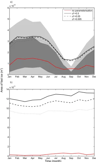
forcf = 0.05 (solid black line) and 0.005 (dashed black line) compared to the standard value cf = 0.5. . . 67 2.25 Area of landfast ice (ms−2) in the (a) Arctic and (b) Antarctic for

cf = 0.5 (solid black line), cf = 0.05 (dashed black line) and cf = 0.005 (dotted black line) compared to the control i.e. no landfast ice parameterisation included (solid red line). Arctic results are plotted

against NIC climatologies of landfast ice area over the time periods

1972-2007 and 1994-2005 in light and dark grey respectively. . . 68

2.26 Observed hourly and averaged 6 hourly wind speed ms−1 at Antarctic

weather station (043166) Lat = 65.5800 N, Lon = 37.1500 W, for hours 10-15 on 08/01/2000 obtained from the Historic Arctic and

Antarctic Surface Observational Data, NSIDC (Stroeve and Shuman,

2004). . . 72

2.27 Arctic annual average ice production (cm day−1) for the a) control (i.e

no parameterisation, b) independent parameterisation and c) anomaly

(independent - control) at 1 degree resolution. Ice production smaller

than 0.001 cm day−1 has been masked to white. . . 75

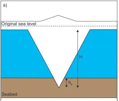
3.1 Effect of tidally induced fluctuations in sea surface height on grounded

ridges where H is draft thickness, hg is the gouge depth and ζt is the

change in sea surface height. . . 86

3.2 The monthly maximum (red) and minimum (blue) sea ice extent

with-out tides (solid line) and with tides (dashed line) for the control

sim-ulation in (a) the Arctic and (b) the Antarctic. In the Arctic the

September extent is used for the minimum in both simulations. . . . 93

3.3 (a) Arctic and (b) Antarctic (i) maximum and (ii) minimum 1997 ice

extent from the NSIDC Sea Ice Index (Fetterer et al., 2002, updated

2009). The pink line represents the monthly median ice extent over

(13)

3.4 Arctic winter (JFM) ice volume per unit area (m) (a) without tides,

(b) with tides, and (c) anomaly (tides-no tides) for the control

simu-lation (i.e. no landfast ice parameterisation). . . 95

3.5 Arctic summer (JAS) ice volume per unit area (m) (a) without tides,

(b) with tides, and (c) anomaly (tides-no tides) for the control

simu-lation (i.e. no landfast ice parameterisation). . . 96

3.6 Annual mean residual tidal currents (m s−1) for the control

simula-tion (i.e. no landfast ice parameterisasimula-tion) at every second grid cell

in the x and y direction (a) the Arctic, and at every second cell

in the x direction only in (b) the Antarctic. The markers X1 and

X2 relate to locations where tidal time series are considered in

Fig-ures 3.12, 3.13, 3.26, 3.27. . . 97

3.7 Arctic mean ice velocity anomaly (tides - no tides) (m s−1) for the

control simulation (i.e. no landfast ice parameterisation) at every

second grid cell in the x and y direction for (a) the winter (JFM) and

(b) the summer (JAS). . . 98

3.8 5 day mean ice volume (m3) for the control simulation (i.e. no landfast

ice parameterisation) without tides (solid black line) and with tides

(dashed black line) for (a) the Arctic and (b) the Antarctic. . . 99

3.9 Arctic mean annual ice thickness distribution per thickness category

without tides (solid line) and with tides (dashed line) for (a) all tested

scenarios, (b) the control, (c) the independent parameterisation, and

the restricted parameterisations for (d)λ = 1.25, (e) λ= 1.10 and (f)

λ= 1.05. Details of thickness category limits can be found in Table 3.1 100 3.10 Annual mean Arctic fractional lead area (0−1) for the control

simu-lation (i.e. no landfast ice parameterisation) (a) without tides and (b)

(14)

3.11 Arctic annual mean ice production (cm day−1) a) without tides and

b) tidal induced anomaly (tides - no tides) using the independent

landfast ice parameterisation. Ice production smaller than 0.001 mm

day−1 have been masked to white. . . 102

3.12 (a) Tidal elevation (m) and (b) fractional area of grounded ice at a

coastal point in the Barents Sea (X1 in Fig. 3.6(a)) for the 1st-3rd

March from Year 11 in the independent parameterisation model run

forced with 1997 atmospheric data. . . 107

coastal point in the Hudson Strait (X2 in Fig. 3.6(a)) for the 1st-3rd

March from Year 11 in the independent parameterisation model run

forced with 1997 atmospheric data. . . 107

coastal point in the Hudson Strait (X2 in Fig. 3.6(a)) for March from

Year 11 in the independent parameterisation model run forced with

1997 atmospheric data. . . 108

3.15 Arctic annual mean transport of grounded ice (ms−1) and normalised

unit vector for the independent parameterisation for a) simulation

without tides and b) anomaly (tides - no tides). In the anomaly tidal

induced changes less than 1×10−10 ms−1 are masked white. . . 109

3.16 Monthly estimates of Arctic grounded ice area without tidal forcing

(solid) and including tidal forcing (dashed) for model experiments run

at 1 degree resolution for the control (red), independent grounding

(blue), and restricted grounding schemes with a coupling parameter

λ = 1.25 (green), 1.10 (cyan) and 1.05 (magenta) for (a) all simula-tions and (b) magnification of the control and restricted

(15)

3.17 Monthly estimates of Arctic landfast ice area without tides (solid line)

and with tides (dashed line) for model experiments run at 1 degree

resolution for the control (red), independent grounding (blue), and

restricted grounding schemes using a coupling parameter λ = 1.25 (green), 1.10 (cyan), and 1.05 (magenta). The light and dark grey shaded bands represent the range in landfast ice area estimated from

NIC climatology over 1972-2007 and 1994-2005 respectively. . . 113

3.18 Arctic landfast ice duration from 5 day averages for model experiments

run at 1 degree resolution including tidal forcing for the (a) control, (b)

independent parameterisation, and restricted parameterisation using

(c) λ= 1.25, (d)λ= 1.10, and (e)λ = 1.05. . . 114 3.19 Arctic landfast ice duration anomaly (tides - no tides) from 5 day

averages for model experiments run at 1 degree resolution for the (a)

control, (b) independent parameterisation, and restricted

parameter-isation using (c) λ = 1.25, (d) λ = 1.10 and (e) λ = 1.05. Red = increase, blue = decrease, white = no change. . . 115

3.20 Antarctic winter (JAS) ice volume per unit area (m) (a) without tides,

(b) with tides, and (c) anomaly (tides - no tides) for the control

sim-ulation (i.e. no landfast ice parameterisation). . . 120

3.21 Antarctic summer (JFM) ice volume per unit area (m) (a) without

tides, (b) with tides, and (c) anomaly (tides - no tides) for the control

simulation (i.e. no landfast ice parameterisation). . . 121

3.22 Antarctic annual mean ice velocity anomaly (tides - no tides) for (a)

the winter (JAS), and (b) the summer (JFM) for the control

(16)

3.23 Antarctic mean annual ice thickness distribution per thickness

cat-egory for (a) all tested scenarios, (b) the control, (c) the

indepen-dent parameterisation and the restricted parameterisations for (d)

λ = 1.25, (e) λ = 1.10, and (f) λ = 1.05 without tides (solid line) and with tides (dashed line). Details of thickness category limits can

be found in Table 3.1 . . . 123

3.24 Annual mean Antarctic fractional lead area (0−1) for (a) without

tides and (b) the anomaly (tides-no tides) for the control simulation

(i.e. no landfast ice parameterisation). Any anomaly less than 0.01 is masked to white to remove noise. . . 124

3.25 Antarctic annual mean ice production (cm day−1) a) without tides,

b) with tide and c) anomaly (tides - no tides) for the independent

landfast ice parameterisation. Ice production smaller than 0.001 mm

day−1 have been masked to white. . . 125

coastal point in the Ross Sea (X1 in Figure 3.6(b)) for the 1st-3rd

September from Year 11 in the independent parameterisation model

run forced with 1997 atmospheric data. . . 129

coastal point in the Bellingshausen Sea (X2 in Figure 3.6(b)) for the

1st-3rd September from Year 11 in the independent parameterisation

model run forced with 1997 atmospheric data. . . 129

3.28 (a) Tidal elevation (m) and (b) fractional area of grounded ice at

a coastal point in the Bellingshausen Sea (X2 in Figure 3.6(b)) for

September from Year 11 in the independent parameterisation model

run forced with 1997 atmospheric data. . . 130

3.29 Antarctic annual mean transport of grounded ice (ms−1) and

nor-malised unit vector for the independent parameterisation for a)

simu-lation without tides and b) anomaly (tides - no tides). In the anomaly

(17)

3.30 Monthly estimates of Antarctic grounded ice area without tides (solid)

and with tides (dashed) for model experiments run at 1 degree

resolu-tion for the control (red), independent grounding (blue), and restricted

grounding schemes with a coupling parameter λ= 1.25 (green), 1.10 (cyan), and 1.05 (magenta) for (a) all simulations and (b) magnifica-tion of the control and restricted parameterisamagnifica-tion. . . 132

3.31 Monthly estimates of Antarctic landfast ice area without tides (solid

line) and with tides (dashed line) for model experiments run at 1

degree resolution for the control (red), independent grounding (blue),

and restricted grounding schemes using a coupling parameterλ= 1.25 (green), 1.10 (cyan), and 1.05 (magenta). . . 135 3.32 Antarctic landfast ice duration from 5 day averages for model

simu-lations run at 1 degree resolution including tidal forcing for the (a)

parameter-isation using (c) λ= 1.25, (d) λ= 1.10 and (e) λ= 1.05. . . 136 3.33 Antarctic landfast ice duration anomaly (tides - no tides) from 5 day

averages for model simulations run at 1 degree resolution for the (a)

parameter-isation using (c) λ = 1.25, (d) λ = 1.10 and (e) λ = 1.05. Red = increase, blue = decrease, white = no change. . . 137

4.1 Schematic showing a) the model domain for the 1D pure compression

scenario and b) the sign and magnitude of the internal ice stress (σpc)

along the central transect (indicated by the dashed red line in (a)).

(18)

4.2 Schematic showing a) the model domain for the 1D pure shear scenario

and b) the sign and magnitude of the internal ice stress (σps) along the

central transect (indicated by the dashed red line in (a)). Here, P∗ = 27500 Nm−2 is the internal ice strength constant (Equation (4.6)),

e= 2 is the eccentricity of the yield curve and h is the ice thickness. 152 4.3 Analytical (black line) and numerical (CICE) (red line) solutions for

(a) the maximum wind stress (Nm−2) under which ice can remain

stationary, and (b) the associated non dimensional characteristic

vari-able, αpc, for ice acting under pure compression. . . 159

4.4 Analytical (black line) and numerical (CICE) (red line) solutions for

(a) the maximum wind stress (Nm−2) under which ice can remain

sta-tionary, and (b) the associated non dimensional characteristic variable

αps for ice acting under pure shear. . . 164

4.5 Schematic showing the model domain for the two dimensional

sce-nario including compressive and shear stress. The central transect is

indicated by the dashed red line. . . 166

4.6 Maximum wind stress at which ice is considered motionless (i.e.

land-fast) for increasing opening widths in the offshore grounded ridges

(L2), for a sheet of ice 200 km wide (red line) and 250 km wide (black

line) initialised at rest. The light and additional dark grey shaded

areas illustrate the model results where are ignored due to unrealistic

fluid like flow for L2 = 250 and 200 km respectively. . . 171

4.7 Maximum wind stress under which landfast ice can form as suggested

by the proposed characteristic variables, τa1 =

P∗h√1+1_/e2

L1 (red line),

τa2 = P

∗_h

eL2 (green line) and τa3 = min(τa1, τa2) (blue line) and the

modelled solution (black line), for an ice cover 250 km wide (solid

(19)

4.8 Value of proposed characteristic variables,α1 = P∗h

√

1+1_/e2

τaL1 (red line),

α2 = P

∗_h

eτaL2 (green line) and α3 = min(α1, α2) (blue line) for an ice

cover 250 km wide (solid lines) and 200 km wide (dashed lines). The

analytically expected solution is shown by the black lines. . . 175

4.9 Maximum wind stress under which landfast ice can form as suggested

by the proposed characteristic variables,τa4 =µ1τaps+(1−µ1)τapc (red

line),τa5 =µ2τaps+(1−µ2)τapc (green line),τa6 =µ3τaps+(1−µ3)τapc

(blue line) and the modelled solution (black line), for an ice cover 250

km wide (solid lines) and 200 km wide (dashed lines). . . 176

4.10 Value of proposed characteristic variables, α4 = µ1αps + (1−µ1)αpc

(red line),α5 =µ2αps+(1−µ2)αpc(green line),α6 =µ3αps+(1−µ3)αpc

(blue line) for an ice cover 250 km wide (solid lines) and 200 km wide

(dashed lines). The analytically expected solution is shown by the

black lines. . . 177

A.1 Schematic showing ice draft and ocean depth versus cell fractional

area (A), where A varies between 0 and 1. In (a) the minimum an-choring strength produced by the grounded ice is illustrated and (b)

the maximum anchoring strength produced by the grounded ice is

il-lustrated. Where h1,2 are the minimum and maximum ice drafts, d1,2

are the minimum and maximum ocean depths, hg is the gouge depth

(20)

List of Tables

2.1 Ice and bathymetry categories . . . 34

2.2 Ice thickness density and cumulative distributions . . . 76

3.1 Difference in total ice area per thickness category (tides - no tides) . . 116

4.1 Model specifications for the one dimensional idealised model domains. 153

4.2 Model specifications for the 2D idealised model domain . . . 167

(21)

Acknowledgements

Firstly, I want to thank all three of my supervisors, Dr Miguel Angel Morales

Maqueda (National Oceanography Centre, Liverpool), Dr Clare Postlethwaite (British

Oceanographic Data Centre) and Dr Harry Leach (University of Liverpool), to whom

I owe a great debt. Their encouragement, advice, endless hours of discussion and

problem solving have been essential to the completion of this thesis. I hope each of

you understand how much you have helped.

The Los Alamos National Laboratory provided the Los Alamos Sea Ice code

(CICE), which was essential to this research. I owe a massive thank you to everyone

who helped me get to grips with this code, develop my own scripts and teach me

to use the NOCL cluster. This includes all 3 of my supervisors, but also Dr Vassil

Roussenov from the University of Liverpool and Mark Birmingham from the NOCL

IT help desk. Thank you for not laughing when I asked stupid questions or made

silly mistakes.

I owe a massive thank you to all my fellow students at the University of Liverpool

and the National Oceanography Centre Liverpool, and in particular my office mates.

Without their help, reassurance, support, and friendship, I do not think I would have

survived.

My last thanks is for my friends and family, in particular my partner Simon, who

have helped me through the last 4 years. It hasn’t been easy, and I am in awe of the

apparently unlimited amount of patience you had for me, and your ability to help

(22)

Chapter 1 Introduction

1.1 Sea ice

Sea ice is a fundamental component of the cryosphere, and an integral part of our

global climate system. It modifies the exchange of heat, gas and momentum between

the atmosphere and polar oceans, it affects the fresh water budget and alters the

albedo of the high latitudes. Most sea ice is part of the mobile pack ice, which

is free to circulate under the influence of winds and oceanic currents. Pack ice is

extremely inhomogeneous with differences in concentration, thickness, age and snow

cover occurring over a range of spatial scales. Landfast ice is a distinct type of sea

ice which is attached to the coast, remains motionless for long periods of time, and

is generally homogeneous in properties.

In recent years, satellite observations have shown a significant decline in Arctic

sea ice extent in all seasons, but most markedly in summer (Stroeve et al., 2012).

The record minimum Arctic ice extent (since 1979) was reached in September 2012,

as reported by the National Snow and Ice Data Centre (NSIDC). This decline in

extent has been accompanied by a reduction in ice thickness (Rothrock et al., 2003;

Schweiger et al., 2011; Laxon et al., 2013). Similar observations in the Antarctic have

not revealed a significantly consistent trend. In order to fully understand the impacts

of the observed and future changes in polar sea ice, it is essential to understand all

(23)

them in global models.

1.2 Landfast sea ice definition

There is no one standard definition consistently applied to landfast sea ice. Some

definitions are based on physical understanding of the landfast ice system while

oth-ers are based more generally on observations and trends. The applied definition,

and how stringent it is, will have implications on the resultant estimates of landfast

ice occurrence. Although definitions can vary significantly, most agree on two

fun-damental characteristics, that landfast ice is stationary, and that it is attached to

the coast or seabed at some point. The World Meteorological Organisation (WMO,

1970) defines landfast ice as “sea ice which forms and remains fast along the coast,

where it is attached to the shore, to an ice wall, to an ice front, between shoals and

grounded icebergs”. This definition was further refined by Mahoney et al. (2005),

who attached a minimum time constraint of 20 days which the ice must remain

stationary for in order to be considered landfast. This time period is long enough

to preclude transient events such as pack ice being temporarily driven shoreward

by oceanic or atmospheric forcing, but short enough to resolve intra-annual events,

such as seasonal growth and breakup of landfast ice. Recent research into landfast

ice has widely adopted the definition proposed by Mahoney et al. (2005) in both

observational and modelling studies, and is the one applied in this research.

1.3 Background

Landfast sea ice, as shown in Fig 1.1, is a recurring feature along many coastlines

in the polar regions. Most landfast ice is seasonal, with only a small proportion

becoming multiyear. The multiyear landfast ice which does occur usually forms as

a result of highly restrictive geometry, such as in the Canadian Arctic Archipelago

(CAA). A prominent example of the semi-permanent landfast ice is the Norske Øer

(24)

Figure 1.1: A Visible Band Image of Beaufort Sea for 04 May 2004 (Eicken et al.,

2009). Leads appear dark, sea ice appears grey, and the Alaskan coast is white. The

landfast ice is that shoreward of the lead.

cover is separated into 3 distinct sections: undeformed ice grown in coastal regions

which is subdivided into bottomfast or floating, and a section of highly deformed

shear and pressure ridges located near the landfast ice edge, known as the stamukhi

zone (Fig.1.2) (Reimnitz, 2000; Mahoney et al., 2007b). The word stamukhi is a

historical Russian term that describes an area of grounded ice (Weeks, 2010). The

stamukhi zone at the edge of the landfast ice cover is discontinuous, meaning that

there are sections of the landfast ice edge which are not dominated by grounded

pressure ridges. The floating section of the landfast ice cover (i.e. ignoring the

stamukhi zone) generally has a homogeneous thickness, as its growth is dominated by

thermodynamics. Tidal cracks are a common occurrence between the bottomfast and

floating sections. They accommodate differential motion between the two sections

caused by changes in sea level (Kovacs and Mellor, 1974b; Reimnitz and Barnes, 1974;

Reimnitz, 2000). The tide cracks are assumed to have negligible tensile strength,

meaning that it is unlikely that bottomfast ice plays a significant role in attaching

(25)

Bottomfast Floating

Stamukhi zone

Pack ice

Seabed

Seaward fast ice edge

Tidal cracks

Sea bed gouge

Figure 1.2: A generalized cross-section of landfast ice extending offshore showing

a grounded pressure ridge (part of the stamukhi zone) at the landfast ice edge.

However, the grounded ice ridges do not occur continuously along the landfast ice

edge.

1.4 Formation

Sea ice forms when the sea water is cooled to the freezing point. The freezing point

of sea water is depressed in comparison to that of fresh water due to the addition

of salt. Typically, in polar regions (with a salinity of 35 ppt) the sea water freezes

at −1.8◦C. Sea ice begins by forming small crystals which join together to form needle like structures, which are typically 3-4 mm in diameter known as frazil ice.

The frazil ice crystals coalesce to form larger structures. If the ice formation occurs

in calm conditions then smooth, thin, homogeneous sheets of ice develop, known as

nilas or grease ice. If the weather conditions are not calm then the frazil ice turns

into circular disks of ice, known as pancake ice. Eventually, the individual ’pancakes’

consolidate into a coherent sheet of sea ice. The thin sheets of ice thicken through

rafting and ridging processes, and continue to grow in winter through congelation to

form first year ice. Congelation is when water molecules freeze onto the underside of

the existing ice cover (Wadhams, 2000). Sea ice which survives one or more summer

melt season is known as multiyear, or perennial ice.

(26)

content, temperature and density. Thin ice fails or breaks more easily under stress.

It is widely accepted that a consolidated sheet of ice is strongest in compression,

then shear, and weakest in tension (Hibler, 1979), with the tensile strength generally

accepted to be around1_/₂₀th _{of the compressive strength (Hibler and Schulson, 2000;}

Wang, 2007). As sea ice is highly fractured at fine scales it is generally assumed to

have no, or negligible, tensile strength at most model resolutions (Lepparanta, 1998).

Recently, there has been some discussion as to whether landfast ice, unlike pack ice,

does in fact contain a significant degree of tensile strength which would allow it

to remain attached along an unrestricted coastline, over relatively deep water, and

under the influence of offshore winds as these conditions mean that it is unlikely that

restrictive geometry plays a significant role in landfast ice creation. Tremblay and

Hakakian (2006) reported that sea ice exhibits tensile strength when subjected to

offshore winds, particularly in the East Siberian Sea. However, to date no definitive

modelling work in support of this theory has been proposed (K¨onig Beatty and

Holland, 2010; ´Olason, 2012).

Landfast ice forms through a number of different processes. Probably the most

well understood is that of restrictive geometry, where ice is held stationary through

resistive shear or compressional stress imparted on the ice as it interacts with narrow

channels or embayments, such as in the CAA. Landfast ice is also observed to occur

along unrestricted coastlines and under the influence of offshore winds. Both of

these factors act to prevent the formation, or encourage the breakup of landfast

ice, raising the question of how it can form under these conditions. Discontinuous

grounded ridges along the landfast ice edge add stability to the fast ice sheet acting to

limit lateral motion. The grounded ridges usually form through offshore deformation

of pack ice but can also form through in situ deformation of the landfast ice itself.

The ridges which form offshore drift inshore under the influence of oceanic and

atmospheric stresses, and ground on shallowing bathymetry. The ridges gouge the

seabed to a given depth until the resistive frictional force imparted by the seabed

(27)

the gouge depends on the strength of the keel, how strongly the ice sheet and ridge

are coupled, and the strength of the seabed sediments (Kovacs and Mellor, 1974a).

The anchoring strength provided by the ridge is limited by either the strength of the

ridge’s keel or its coupling with the seabed i.e. the gouge depth. Grounded ridges

which form in situ are thought to provide significantly lower anchoring strengths

than those which form offshore as they typically only reach thicknesses just equal to

the local ocean depth, and so are not strongly coupled with the seabed (Mahoney

et al., 2007b; Phillips et al., 2005).

Landfast ice begins to form at the coast, gradually advancing offshore until a stable

extent is reached, the location of which is primarily determined by the coastline and

bathymetry (Mahoney et al., 2007a). This occurs in early winter once the thick

ridges have assimilated into the shallow coastal regions. Once the stable extent

is reached, the landfast ice is persistent, generally remaining unchanged until the

summer melt season. Episodic breakout events do occur, where the fast ice edge

temporally extends beyond the stable width, but these are generally short lived.

In late spring, with the onset of thawing temperatures, the landfast cover breaks-up

and drifts offshore. The floating section is thinned thermodynamically and weakened.

Once the grounded ridges uncouple from the seabed the landfast ice sheet breaks-up

and drifts offshore rather than melting in situ. This process is much quicker than

the formation, and in many cases the landfast ice is completely removed within a few

days. Recent observations have shown a reduction in landfast sea ice in the Arctic

(Mahoney et al., 2007a). This reduction has been attributed to the earlier onset of

thawing temperatures in spring and the later inclusion of the ice ridges into shallow

coastal waters in winter due to an increased northward retreat of the perennial ice

edge (Serreze et al., 2003; Stroeve et al., 2005).

In general, Arctic landfast ice is observed to reach its stable extent around the

20 m isobath (Kovacs and Mellor, 1974b; Reimnitz and Barnes, 1974; Stringer, 1974;

Stringer et al., 1980; Mahoney et al., 2007a), but this can differ between regions.

(28)

10 m isobath, while in the eastern Kara sea the landfast ice edge can stabilise around

the 100 m isobath (Divine et al., 2004). These variations occur for a number of

reasons. For example, the occurrence of offshore islands can allow landfast ice to

form in regions which are much deeper than 20 m. Also, if local ice deformation

results in ridges which are relatively shallow (less than 20 m), then the landfast ice

edge can only extend to regions which are shallower than the 20 m isobath. Strong

variations in landfast ice width are also observed due to differences in the slope of the

continental shelf, as this determines how far offshore the ridges will ground. Landfast

ice is observed to extend hundreds of kilometres from the coast in the Siberian Arctic

(Barnett, 1991; Eicken et al., 2005), while along the Alaskan coastline it generally

reaches stable widths of ≤ 50 km (Stringer et al., 1980). The strong correlation

between the stable landfast ice edge and the 20 m isobath suggests the importance

of grounded ridges in landfast ice formation and retention. Ice ridges, which are

formed through the convergence of the sea ice cover, commonly reach thicknesses of

20 m in the Arctic, although thicker ice ridges have been observed (e.g. Barnes et al.,

1984; Timco and Burden, 1997). The maximum thickness of an ice ridge is limited,

as once a ridge has reached a certain vertical length, the pack ice which surrounds

the ice is too weak to penetrate the ridge under deformation to allow it to grow

thicker. At this point, the ice cover will break in front of the ridge, and the ridge will

grow laterally (Lepparanta, 2011; Hopkins et al., 1991). This maximum thickness

limit is primarily controlled by the thickness of the parent ice cover, while also being

dependent on the strength of the convergent stresses acting on the ice cover and the

duration over which the convergent stresses act. The thicker the starting ice cover,

the stronger the convergent stresses, and the longer these stresses occur, the thicker

the resultant ice ridge will become. Much of Arctic sea ice does not commonly exceed

thermodynamically driven thickness of 2-3 m (Rothrock et al., 2003; Schweiger et al.,

2011; Laxon et al., 2013). As such, the maximum thickness of the pressure ridges

will be capped by this (along with the strength of the convergent stresses and the

timescale over which these are applied). In the Arctic, this results in ridges which

(29)

The occurrence of landfast ice in the Antarctic is controlled by the same processes

as in the Arctic but significant differences in the physical environment have resulted

in notable differences in the resultant landfast ice. Much of the continental shelf

surrounding the Antarctic continent is generally much deeper than in the Arctic,

beyond depths which sea ice ridges would be able to ground in. The lack of grounded

ridges will act to limit landfast ice formation. However, the occurrence of very

thick icebergs, up to ≈ 400m (Massom et al., 2001), provide anchoring points for

the landfast ice in very deep water. The occurrence of extensive ice sheets over

the available continental shelf, and strong katabatic winds, both act to limit the

grounding of ridges and the formation of landfast ice. Limited studies of Antarctic

fast ice have meant that long term or large spatial scale records of landfast ice are

significantly lacking. Along the east Antarctic coast landfast ice is known to form in

narrow bands of varying widths rarely exceeding 150 km (Giles et al., 2008).

1.5 Importance

Landfast ice is an important component of the cryosphere, influencing a wide range

of local and global processes. Due to its persistence and lack of mobility, landfast ice

acts as an extension of the coast over the continental shelf, fundamentally modifying

the exchange of heat, gas, and momentum between the atmosphere and ocean. This

is unlike pack ice which has the ability to move, allowing the ocean and atmosphere

to intermittently interact with one another.

Latent heat polynyas form offshore of many coastlines in the polar regions. The

large negative ocean to atmosphere heat fluxes (up to several hundred Wm−2) affect

mesoscale atmospheric motion (Dethleff, 1994) and ocean circulation (e.g.

Morales-Maqueda et al., 2004). High rates of ice production caused by the negative heat

flux result in high levels of brine rejection, altering the local ocean salinity. This

process sets up vertical mixing and convection which can result in the formation and

cascading of intermediate and deep water masses. The properties of the dense water

(30)

the formation polynya. The occurrence of landfast ice moves the effective coastline,

and the location of the flaw polynyas, offshore. The dense water then has a reduced

distance to travel before reaching the shelf break, undergoing less mixing with the

fresher ambient shelf water. This allows the water to retain a density close to its

original maximum and cascade to great depths, forming deep water (Schauer and

Fahrbach, 1999).

Landfast ice is the form of sea ice which people have most frequent and direct

contact with. The landfast ice edge is an essential habitat and feeding ground for

Arctic mammals and the Inuit who depend on them for subsistence (Druckenmiller

et al., 2000). It also affects economic activities such as shipping and offshore oil and

gas exploration. With increased shipping and mineral exploration interest in Arctic

coastal waters, understanding the landfast ice system and being able to accurately

model it is becoming increasingly important.

1.6 Research aims

Despite the important and wide ranging effects of landfast sea ice, there has been

limited work into its accurate inclusion in dynamical models. Landfast ice modelling

studies originally concentrated on thermodynamic models. These thermodynamic

studies considered ice to be landfast when the ice thickness would reach, or exceed,

a given percentage of the local ocean depth (usually 10%) (Flato and Brown, 1996;

Dumas et al., 2006; Lieser, 2004). More recently, work has focused on producing a

dynamic representation of landfast sea ice. However, to date, dynamic sea ice models

have not been able to reproduce landfast sea ice in a realistic setting. K¨onig Beatty

and Holland (2010) showed that by adding tensile strength into a commonly used sea

ice model they were able to produce landfast sea ice features in idealised scenarios.

Tensile strength allows the ice to remain attached to an unrestricted coastline, under

forcing conditions acting to set the ice into motion. It is commonly accepted that,

in general, sea ice has no, or a very little, tensile strength as it is highly fractured

(31)

as to whether landfast ice contains a degree of tensile strength. K¨onig Beatty and

Holland (2010) found that the magnitude of tensile strength required to simulate

landfast ice was equal to the compressive strength of the ice, which contradicts what

is known about the strength of sea ice; that ice is strongest in compression, then

shear, and weakest in tension (Hibler, 1979). K¨onig Beatty and Holland (2010) were

also unable to reproduce landfast ice features under realistic conditions.

Landfast ice research has generally focused on regional scales, due to the increases

in model resolution that can be gained. One region which has been studied in detail,

with respect to landfast sea ice is the Kara Sea, building up a good understanding of

the seasonal progression of the landfast ice and the processes involved in its formation

(Volkov et al., 2002; Divine et al., 2004, 2005). As such, the Kara Sea has become

a good case study for testing modelling concepts. ´Olason (2012) followed a similar

method to that proposed by K¨onig Beatty and Holland (2010), modelling landfast ice

in the Kara Sea by allowing the sea ice to contain a degree of tensile strength. The

spatial distribution of the modelled landfast ice compared well with observations,

but the model was not able to realistically represent the duration of the fast ice

cover, despite modelling at relatively fine resolutions.

In this study we consider the inability of sea ice models to produce realistic

landfast sea ice along unrestricted coastlines and under offshore winds, when it is

observed to occur in reality. In contrast to recent landfast ice studies carried out

by K¨onig Beatty and Holland (2010) and ´Olason (2012) we propose that it is not

tensile strength within the landfast ice which allows it to remain fast under offshore

winds and along unrestricted coastlines. Instead, we consider the hypothesis that

the grounded ridges within the stamukhi zone (at the offshore edge of the landfast

ice cover) provide enough lateral stability to keep the ice fast.

The formation and properties of thick ice ridges has been widely studied over the

years (Lepparanta and Hakala, 1992; Lepparanta et al., 1995; Timco and Burden,

1997). The impact of these ice ridges on the seabed, i.e. seabed gouging, has also

been of significant interest, particularly in relation to the location and depth of oil

(32)

The impact of the thick ice ridges on the formation and maintenance of landfast ice

formation and maintenance has not been widely investigated.

This study begins with a discussion of how ridges help to form landfast ice,

and important aspects relating to this process. Chapter 2 considers two separate

methods of parameterising grounded ridges, and their impact on the ice cover, in a

sea ice model. We then test the ability of the parameterisations to reproduce the

formation, maintenance and breakup of landfast sea ice in the Arctic and Antarctic.

We investigate the impact of tides on grounded ridges, and consider the sensitivity

of the modelled landfast ice to realistic tidal forcing in Chapter 3. We finish by

considering some open questions remaining in landfast ice research, and consider

whether we can use a model representation of landfast ice to better understand the

sensitivity of the physical landfast ice system. That is, is it possible to use models

to better understand the physics of the landfast ice system, such as under what

(33)

Chapter 2 Modelling landfast ice production

due to grounded ice

2.1 Introduction

Landfast sea ice is separated into 3 distinct sections; undeformed ice grown in coastal

regions which is subdivided into bottomfast or floating, and a section of highly

deformed shear and pressure ridges located near the landfast ice edge, known as

the stamukhi zone (Fig.1.2). The resultant frictional drag force exerted on the ice

due to contact with the sea floor causes the thick ridges to slow, and in some cases

completely arrest (Fig.2.1), a process known as grounding. The grounded ridges

then act as pinning points within the landfast ice cover, limiting lateral movement

of the adjacent ice. The landfast ice sheet begins to form in early winter, once the

thick ridges have assimilated into the shallow coastal regions. In spring/summer

the landfast ice cover does not typically melt in situ. Instead, the grounded ridges

uncouple from the seabed due to a combination of thermodynamic melt and offshore

wind forcing. This allows the weakened landfast ice to detach from the coast and drift

offshore. This process can be quite dramatic, happening over a few days. Grounded

ice ridges thus play an integral role in the formation, maintenance and break-up of

landfast sea ice.

(34)

Sail

Keel Waterline

Seabed

σsb

h H

hg

Figure 2.1: An idealized cross-section of a grounded ridge where draft ice thickness

(H) is a fraction (ρi

ρw) of the total ice thickness (h). The water and ice densities are

given by ρw and ρi respectively. The ridge has gouged the seabed to a depth of hg,

and exerts a shear stress (σsb) at the seabed.

determined. The parameters important in determining the amount of ice aground

are the draft ice thickness and ocean depth. If the draft ice thickness is greater than

the ocean depth then the ice will ground. In this Chapter we explore methods of

parameterising the sub-grid scale occurrence of grounded ridges and the anchoring

strength it provides to the sea ice cover to produce landfast ice.

2.2 Identifying grounded ice

For a simple idealised scenario, or when the model resolution is fine enough that

within each grid cell ice draft and ocean depth are unique, the draft ice thickness and

ocean depth are independent. That is, the amount of ice in contact with the seabed

will remain unchanged irrespective of how either variable is spatially distributed

(35)

and a parameterisation to determine the sub-grid scale area of grounded ice is not

required. However, it is generally unrealistic to run models at fine enough resolution

such that the variables are unique.

When variables are multi-category and the sub-grid scale distribution of either

variable is unknown, as they are in most sea ice modelling studies, then within

each grid cell a method of determining the area of ice in contact with the seabed is

necessary. Figure 2.2 shows a grid cell with ice thickness and ocean depth of two

categories. For this case there are only two possible ways that the ice can be spatially

distributed with respect to the bathymetry. Therefore the resultant area of grounded

ice can again be logically determined. In the first example (a) the area of grounded

ice is equal to the difference between the area of shallow bathymetry and the area of

thin ice (Ag =Ad1−Ah1). This is the minimum amount of ice that necessarily must

be aground. In the second example (b) the area of grounded ice is equal to the area

of shallow bathymetry (Ag =Ad1). This is the maximum possible area of grounded

ice. However, as the number of ice thickness and ocean depth categories increases

so too does the complexity of the solution. At resolutions that sea ice is generally

modelled at the number of ice and ocean categories within a standard grid cell is

such that the solution can not be determined logically. In this case a method, or

parameterisation, to determine the sub-grid scale occurrence of grounded ice must

be used.

Multi-category draft ice thickness (H) and ocean depth (D) can be considered as

continuous random variables, with probability density functions (PDFs) f(h) and

g(d) respectively,

P(0≤ H ≤ ∞) =

Z ∞

0

dh f(h) = 1, (2.1)

P(0≤ D ≤ ∞) =

Z ∞

0

dd g(d) = 1. (2.2)

The draft ice thickness (H) is the thickness of ice underwater, where H = ρi

ρwh and

(36)

d1

d2 h2 h1

a) Minimum

d1

d2 h2

h1 b) Maximum

hg

dg

Seabed Seabed z

A

z

A

hg

Figure 2.2: Schematic showing ice draft and ocean depth versus cell fractional area

(A), where A varies between 0 and 1, for ice thickness (h1,2) and ocean depth (d1,2)

of two categories. The ice can be distributed within the grid cell in two ways ((a)

and (b)) which results in different amounts of grounded ice. The red line indicates

the area of grounded ice, Ag, and hg is the depth to which the ice can gouge the

(37)

value in a given interval. In this case the PDFs for ice thickness and ocean depth

represent the probability that the ice will be a certain thickness or the ocean will be a

certain depth. In Equation (2.2) g(d) is only considered over positive depth ranges, as land values are assumed to be 0. The PDF for ice thickness and ocean depth

can then be joined (known as a joint probability density function (JDF)) to find the

probability that the ice thickness and ocean depth both take on certain values,

P(0≤ H ≤ ∞,0≤ D ≤ ∞) =

Z ∞

0

dh

Z ∞

0

dd j(h, d) = 1. (2.3)

The JDF can be used to find the probability that ice will be aground by finding the

probability the ice will be thicker than ocean depth. When the JDF is constructed

assumptions need to be made about the continuous random variables being joined.

These assumptions are important as it will affect the final solution. We do not have

sufficient understanding of the physics of the landfast ice system to determine a

realistic, dynamically based, joint distribution. It may be useful to mathematically

determine the solution bounds by finding the joint distribution which produces the

minimum and maximum anchoring strength produced by the grounded ice. The

realistic solution must then fall between these extremes. Further details on this are

included in the Appendix A.

The simplest approach would be to define a joint distribution based on the

as-sumption that the ice draft and ocean depth are independent, as they are in the

single category case discussed earlier. This assumption places no restriction on the

sub-grid scale distribution of either variable; within a model grid cell ice can ground

anywhere where it is thicker than the ocean depth. The main limitation of this

method is that it permits the occurrence, and grounding, of erroneously thick ice on

shallow bathymetry. A more restrictive joint distribution could be defined, where

the user places restrictions on the sub-grid scale distribution of one, or both, of the

(38)

2.3 Landfast ice parameterisation

In this analysis we produce two landfast ice parameterisations which account for

the sub-grid scale grounding of thick ice ridges, and the anchoring strength they

impart on the landfast ice cover. We begin by producing a JDF from PDF’s of

ice draft and ocean depth assuming an independent relation between ice draft and

ocean depth. Advancing from this an alternative parameterisation is defined which

restricts the independently produced joint distribution by limiting the maximum ice

draft to ocean depth ratio for grounded ice.

2.3.1 Independent joint density function

As previously discussed, a JDF can be defined from the PDFs of two continuous

random variables. If the continuous random variables are independent then the JDF

is defined as j(x, y) = f(x)×g(y). As such, by assuming that ice thickness and ocean depth are independent, the associated JDF is

j(h, d) = f(h)×g(d), (2.4)

wheref(h) andg(d) are the probability density functions for ice thickness and ocean depth respectively. For example, if a grid cell is completely covered in ice which

is uniformly distributed across all thickness categories, that is, there is the same

amount of ice within each thickness category,

f(h) =





 1_/₂_h

m if 0≤h ≤2hm,

0 otherwise,

where 2hm is the maximum ice thickness andhm is the average ice thickness. This is

illustrated in Figure 2.3 (a). If that same grid cell also contained bathymetry with

(39)

g(d) =





 1_/₂_d

m if 0≤d≤2dm,

0 otherwise,

where 2dm is the maximum ocean depth and dm is the average ocean depth

(illus-trated in Figure 2.3 (b)). Assuming that ice thickness and ocean depth are

indepen-dent the joint distribution, for this example, is therefore

j(h, d) =





 1_/₍₂_h

m×2dm) if 0≤h≤2hmand 0≤d≤2dm,

0 otherwise.

This is illustrated in Figure 2.3 (c).

The JDF can then be used to define the probability that within a grid cell ice

draft is greater than or equal to the ocean depth, and therefore ice can be aground.

The fractional area of grounded ice within each grid cell,AG, is found by integrating

the independent JDF over the probability space that represents a draft thickness

(H) equal to or larger than the ocean depth (d),

AG= Z ∞

0

dh

Z H

0

dd j(h, d). (2.5)

For the example discussed, the area of grounded ice is therefore

AG= Z 2hm

0

dh

Z H

0

dd1_/₍₂_h

m×2dm). (2.6)

To determine the anchoring strength the grounded ice provides to the landfast sea ice

the buoyancy corrected thickness of the grounded ice, HG, is found. It is determined

by multiplying the fractional area of grounded ice by the buoyancy corrected ice

thickness, (h− ρw

ρid),

HG = Z ∞

0

dh

Z H

0

ddh− ρw

ρi

dj(h, d). (2.7)

(40)

[image:40.612.240.412.67.602.2]

Figure 2.3: Probability density function for (a) ice thickness, f(h), and (b) ocean depth, g(d), which are both uniformly distributed across the thickness/depth cate-gories and (c) the associated joint density function, j(h, d), formulated by assuming ice thickness and ocean depth are independent. Here, 2hmand 2dmare the maximum

(41)

HG = Z 2hm

0

dh

Z H

0

ddh−ρw

ρi

d1_/₍₂_h

m×2dm). (2.8)

Assuming an independent relation between ice draft and ocean depth means that

all ice in contact with the seabed is considered aground. The limitation with this

method is that it allows for erroneously thick ice to ground on shallow bathymetry.

This is unrealistic and so the production of grounded ice is expected to be positively

skewed towards higher values.

2.3.2 Restricted joint density function

Restricting the maximum ice draft to ocean depth ratio of grounded ice will reduce

the main limitation of the independent parameterisation, by preventing erroneously

thick ice occurring and grounding on shallow bathymetry. A cap on the maximum

thickness the grounded ice can reach based on seabed gouging is incorporated into

the parameterisation. Seabed gouging is a large-scale coastal process, occurring in

both the Arctic and Antarctic, where the keel of an ice ridge comes into contact with

the seabed. If the resistive force applied to the ice bottom is not able to overcome

the driving forces then the keel will gouge the seabed as shown in Figure 2.1. Gouge

dynamics vary according to the physical geometry of both the ice ridge and the

seabed, but in general the seabed will be displaced laterally to form side berms, and

ahead of the ridge to form a front mount (Barrette, 2011). The depth of the gouge

depends on the strength of the keel, how strongly the ice sheet and ridge are coupled,

and the strength of the seabed sediments (Kovacs and Mellor, 1974a). Multiyear

keels are known to produce the deepest gouges due to the increased strength of the

keel. Gouge intensity in the Arctic is greatest around the 20 m isobath, coinciding

with the seaward location of the landfast ice edge where 1st year shear and pressure

ridges are known to form (Barnes et al., 1984; Hill et al., 1991; Mahoney et al., 2005,

(42)

Limiting the maximum grounded ice thickness

Ice has the ability to gouge the seabed, and effectively increase the local water

depth. The maximum thickness of ice which can ground in a given water depth is

therefore controlled by the ability of the ridge to gouge the seabed. This process is

parametrised here by introducing a coupling parameter λ. Ice is considered aground if it is thicker than the ocean depth and shallower than λ times the ocean depth,

D≤H ≤λD, (2.9)

where D is the ocean depth and

λ= D+hg

D = 1 +

hg

D, (2.10)

where hg is the gouge depth. λ was chosen to be a constant factor as observations

showed that the gouge depth generally increased proportionally to increasing water

depth in the near coastal zone. It is unknown as to why exactly this occurs, but it

seems logical that thicker, and stronger, ice will more likely reside in areas of deep

water, meaning that the seabed is more likely to be gouged to a greater depth. It

is also speculated that reworking by ocean and tidal currents in the shallow water

leads to infilling of the gouges (Barnes et al., 1984; Shapiro and Barnes, 1991). In

the Arctic, for water depths ≤ 20 m observed gouge depths are typically ≤ 1 m

relating to an average coupling parameter λ = 1.05 (Shapiro and Barnes, 1991; Barnes et al., 1984; Reimnitz et al., 1972; Hequette et al., 1995; Conlan et al., 1998).

More extreme gouge depths, 2−3 m, have been observed in equivalent water depths

relating to 1.1≤ λ ≤ 1.15 (Shapiro and Barnes, 1991; Hequette et al., 1995). This parameterisation is likely to be an oversimplification as the gouge depth will depend

on a variety of factors including the geology of the seabed, the strength of the ice

ridge, the strength to which the ridge is coupled to the surrounding ice cover and

the strength of the wind or ocean forcing acting on the ice ridge. For example, if the

(43)

seabed to a greater depth than if the seabed is made up of tightly packed material.

Similarly, the stronger the ice ridge the greater it’s ability to gouge the seabed.

The area and buoyancy corrected thickness of the grounded ice, Equations (2.5)

and (2.7), were modified accordingly to include this additional grounding restriction:

AG = Z ∞

0

dh

Z H

H/λ

dd j(h, d), (2.11)

HG= Z ∞

0

dh

Z H

H/λ

ddh−ρw

ρi

dj(h, d). (2.12)

2.4 Modifying ice motion

In the previous section, a method of identifying the sub-grid scale area and thickness

of grounded ice was developed. Here, a mechanism to modify the velocity of the

grounded ice is discussed. A reactive grounding force per unit area due to the

frictional coupling between grounded ice and the seabed, −F→G, is introduced into

the standard sea ice momentum equation. As a reactive force, it acts to oppose

ice motion and cannot act to enhance or excite new ice motion. The simplified

momentum equation is

m d~u

dt =

−→

FA+ −→

FG, (2.13)

where −F→A encompasses all original forces acting on the ice (as detailed in Equation

(4.1)). The new reactive grounding force, −F→G, is defined as

−→

FG=− − →

U

|−→U|min[M, σsb], (2.14)

where −→U is ice velocity, σsb = ρigHGcf is the shear stress between the ice and the

seabed and M = ρih

Tf |

− →

U| is the maximum frictional force needed to fully arrest the ice in a time scale, Tf. Here, ρi is the density of the ice, g is gravity, HG is the

(44)

seabed. In these experiments the coefficient of friction was taken as cf = 0.5 fromin situ experiments carried out by Shapiro and Metzner (1987) where ice blocks were

dragged along the beach to determine the static and kinetic friction between the

ice blocks and the ground. Using a constant coefficient of friction is likely to be an

oversimplification, as in reality the coefficient of friction will depend on a range of

factors including smoothness of the seabed and ice bottom. As such, it would be

expected to be variable in space and time.

It should be noted that the definition of σsb =ρigHGcf means that its magnitude

is large in comparison to the other dominant stresses acting on the ice i.e. wind

and ocean stress. Considering a typical wind stress in the Arctic of 0.1 Nm−2 and assuming that the buoyancy corrected thickness of the grounded ice (HG) is 1 cm

and cf = 0.5, then the magnitude of σsb ∼ 50 Nm−2 >> 0.1 Nm−2. This suggests

that once ice is aground it is very stable, and almost impossible to uncouple from

the seabed through dynamical processes alone.

2.5 Model description

The Los Alamos Sea Ice Model (CICE) v4.1 was used in this study. The major

components of CICE are the horizontal transport routines, the thermodynamics and

the dynamics which describe the physical state and motion of the ice cover. The

model is fully described by Hunke and Lipscomb (2010), with the key components

detailed here.

2.5.1 Ice thickness distribution

Sea ice is a mixture of open water, thin first year, thicker multiyear and thick shear

and pressure ridges. Both the thermodynamic and dynamic properties of the ice

pack depend the thickness of the ice cover. CICE is a multicategory ice thickness

sea ice model. That is, for each model grid cell CICE determines how much ice

resides in the discrete ice thickness categories. In these experiments the number

Numerical modelling of landfast sea ice