Modelling network travel time reliability under stochastic demand

This is a repository copy of Modelling network travel time reliability under stochastic demand.

White Rose Research Online URL for this paper: http://eprints.whiterose.ac.uk/2471/

Article:

Clark, S.D. and Watling, D.P. (2005) Modelling network travel time reliability under

stochastic demand. Transportation Research B: Methodological, 39 (2). pp. 119-140. ISSN 0191-2615

https://doi.org/10.1016/j.trb.2003.10.006

[email protected] https://eprints.whiterose.ac.uk/ Reuse

See Attached Takedown

If you consider content in White Rose Research Online to be in breach of UK law, please notify us by

White Rose Research Online

http://eprints.whiterose.ac.uk/

Institute of Transport Studies

University of Leeds

This is an author produced version of a paper published in Transportation Research B. This paper has been peer-reviewed but does not include final publisher pagination and formatting.

White Rose Repository URL for this paper: http://eprints.whiterose.ac.uk/2471/

Published paper

Modelling Network Travel Time Reliability

Under Stochastic Demand

Stephen Clark & David Watling1

Institute for Transport Studies, University of Leeds, Woodhouse Lane, Leeds LS2 9JT, U.K.

Revised and resubmitted October 8th 2003

Abstract – A technique is proposed for estimating the probability distribution of total

network travel time, in the light of normal day-to-day variations in the travel demand

matrix over a road traffic network. A solution method is proposed, based on a single

run of a standard traffic assignment model, which operates in two stages. In stage one,

moments of the total travel time distribution are computed by an analytic method,

based on the multivariate moments of the link flow vector. In stage two, a flexible

family of density functions is fitted to these moments. It is discussed how the

resulting distribution may in practice be used to characterise unreliability. Illustrative

numerical tests are reported on a simple network, where the method is seen to provide

a means for identifying sensitive or vulnerable links, and for examining the impact on

network reliability of changes to link capacities. Computational considerations for

large networks, and directions for further research, are discussed.

1

1. INTRODUCTION

Transport planning has been historically concerned with travel behaviour and the

transport system in some nominally ‘typical’ conditions. The emerging topic of

transport network reliability has begun to challenge this ideology. While the initial

impetus appears to have derived from the study of major natural events – such as

earthquakes (Bell & Iida, 1997) – affecting the ‘connectivity’ of a road network, it has

had a wider impact on the thinking of the way in which less severe, but more

frequently-occurring, events may affect the operation of a network. These events

include minor accidents, on-street parking violations, snow, flooding, road

maintenance and traffic signal failures, all of which would lead to variations in link

capacities or free-run speeds. In addition, daily variations in activity patterns,

manifested in the Origin-Destination (O-D) trip matrix, mean that the flows on the

roads also have a major part to play in explaining variations in network performance.

If planners were able to quantify the impact on variable network performance of such

elements, then it would open the possibility of directing both the design (Asakura et al, 2001) and economic appraisal (Du & Nicholson, 1997) of transport policy measures toward an improved treatment of such uncertainty. A practical need

therefore arises for the development of modelling techniques that are able to quantify such impacts. In response to this need, there has been considerable activity in

developing a diverse range of techniques, with five broad classes that may be

identified.

The first class comprises connectivity reliability methods (Bell & Iida, 1997; Asakura

et al, 2001), whereby each link of a network is assumed to have an independent, probabilistic, binary mode of operation. This binary mode may be open/closed, or

may more generally reflect some subjective definition of the successful function of a

link, such as the flow to capacity ratio being less than some given value. The

objective is to compute the probability that a particular path or O-D movement will be

‘connected’, or more generally will ‘function’ as desired.

whereby a continuous probabilistic treatment is made of link, and hence path, travel

times. For example, Asakura & Kashiwadani propose a simulation-based method for

examining the impact of variability in O-D demand levels, whereby an O-D demand

matrix is sampled and an equilibrium assignment performed for each sampled

demand. Bell et al (1999) used a similar philosophical approach, but used equilibrium sensitivity analysis to overcome some of the computational overheads. The

philosophy underlying the methods of Du & Nicholson (1997) is again broadly

similar, but with a specific focus on network degradations in a multi-modal context.

Like Bell et al, Du & Nicholson employ differential sensitivity analysis to their (multi-modal) equilibrium model, in this instance to examine the sensitivity of

equilibrium ‘system surplus’ (a measure of performance of a multi-modal system) to

various unreliable events, such as capacity degradation.

The third class encompasses methods to study capacity reliability (Chen et al, 2000, 2002; see Yang et al, 2000, for a comparison with travel time reliability methods). For example, in Chen et al (2000) the problem is to determine the maximum global O-D matrix multiplier such that the resulting link flows when assigned are within their

respective link capacities. They also discuss how in the lower level (route choice)

problem, an allowance may also be made for the risk-taking approach of drivers in the

assignment model. In Chen et al (2002), alternative notions of reliability are examined in the context of variations in link capacities, using sensitivity analysis to estimate the

impact of a perturbation on equilibrium flows. They also extend this approach by

mixing it with Monte Carlo simulation, in order to estimate sensitivities under more

complex model assumptions such as correlated link capacities.

The fourth class consists of behavioural reliability methods, whereby an effect on mean network performance is presumed to arise from the modified, mean behaviour

of drivers in their attitude to the unpredictable variation and/or the ‘risks’ perceived.

The issue is then how to represent, in an equilibrium framework, the impact on the

‘typical’ route choice pattern (Mirchandani & Soroush, 1987; Lo & Tung, 2000; Yin

The fifth and final class consists of methods to examine the potential reliability of a network; rather than aiming to model performance based on some defined

probabilistic model, these are ‘pessimistic’ methods that aim more to identify

potential weak points/problems and their effect. In this context, Berdica (2001, 2002)

proposed various simple tests of network vulnerability, to examine the impact on various output measures (in equilibrium) to changes in the input variables to a

network model. D’Este & Taylor (2001) likewise considered notions of vulnerability,

with a network node considered vulnerable if the loss of a small number of links

significantly diminishes the ‘accessibility’ of the node. Bell (2000) and Bell & Cassir

(2002) avoided the difficult issue of defining performance probabilities by supposing

that they arose from a ‘game’ between the drivers and an evil entity, suggesting they

could be used as a cautious basis for network design when users are pessimistic about

the performance.

The technique to be proposed in the present paper falls within the class of travel time

reliability methods, specifically examining the impact of variable O-D demand flows

on network performance. As we shall see, however, the approach differs in

philosophical foundation to previous studies of reliability⎯specifically in its use of

the equilibrium paradigm⎯as well as in its solution technique, relying neither on

sensitivity analysis nor Monte Carlo simulation, and in aiming to reconstruct a full

probability distribution for the network performance measure.

2. FRAMEWORK FOR NETWORK RELIABILITY ASSESSMENT

The proposed method is based on an original modelling approach for representing

variable network performance under stochastic O-D demands (to be described in §3),

placed within a framework for reliability assessment. The purpose of the present

section is to describe this latter framework, which is supposed to have a number of

elements:

1. Planning state. The planning state is a representative set of assumptions concerning the state of the road network and demand data that is chosen subjectively by the

planner, for the purpose of devising transport policy and traffic control measures. For

weekday peak-hour when there are no public holidays or special events, and assuming

a network where all links have the potential to operate at their full capacity.

2. Performance measure. This is a scalar measure used to describe the operation of the complete network or of prescribed elements of the network. Without loss of

generality, to simplify later discussions, we suppose the measure is defined so that

larger values of the measure are generally undesirable. For example, on a

network-wide level, we might use proxies for congestion, such as total network travel time of

all drivers or the negative of average network speed, or measures of total fuel

consumption or pollution.

3. Critical value. Recall that we assume the performance measure to be defined such that large values are undesirable. The critical value is a pre-specified value of the

performance level, above which the network would be considered to be performing

“unreliably”, relative to the planning state. A special case is where the critical value is

exactly equal to the value of the performance measure in the planning state: any

performance poorer than the planned situation is then considered subjectively

unreliable. More generally we may define the critical value as some percentage excess

of the value of the performance measure in the planning state.

4. State distribution. The state distribution is a joint density / probability distribution, describing the possible O-D demand and road network states that may actually

prevail. In particular, this distribution can be used to infer the probability distribution

for link flows and travel times across the network, and thereby the probability

distribution of the performance measure.

Combining elements 1 and 2, we then suppose that we have a network model that is

able to estimate the value of the performance measure in the planning state2. From

this value, we define the critical value in 3 as an absolute or percentage excess of the

value in the planning state. In parallel, combining elements 2 and 4 with the network

model yields a probability distribution for the actual values of the performance

measure. This distribution may then be compared with the critical value, and

2

summary measures relating to the critical value produced, e.g. probability of

exceeding critical value, mean performance value when critical value exceeded.

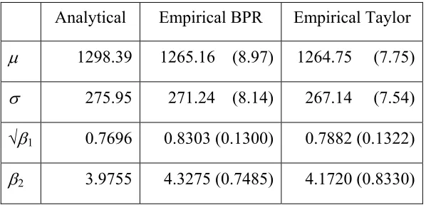
[FIGURE 1 HERE]

In Figure 1 we illustrate such a case, for an example where the performance measure

is a network-wide, continuous attribute. The probability distribution of the actual

values of the performance measure is illustrated. The planning state occurs when the

performance measure equals the mode of around 1; the critical value is defined as a

tolerance of 400% above the performance measure value in the planning state,

yielding a critical value of 5. Then we could define unreliability, for example, in terms of the probability of exceeding the critical value , i.e. the area under

the curve in the range labelled ‘degraded performance’. So in percentage terms we

might say the reliability is

) 5 Pr(M >

(

1 Pr( 5)

)

% 100 − >

= M .

Clearly, the critical value has an important role to play in this measure, yet it will

typically be difficult to justify objectively testing against a single such value. More usefully, then, the reliability could be assessed by reporting such a probability

corresponding to a number of critical values, or by reporting standard upper quantiles

of the distribution, or ultimately by reference to the complete upper tail of the

performance measure distribution. Thus, the motivation in the present paper will be to

reconstruct the full distribution, to provide the maximum information for such an

assessment. This may be contrasted with methods in which the objective is to

compute a single reliability value, in which case more efficient computational

techniques may be available.

For any specific reliability analysis, a first step is therefore to define the performance

measure to be used. Looking to the literature, Bell & Iida (1997) define it from the

road user’s perspective as ‘the probability that a trip can reach its destination within a

given period’. Such a definition may be applied at the path or O-D level. Asakura &

Kashiwadani (1991) suggest an alternative definition to be ‘the upper limit of travel

time by which one can travel … for given probability’. The focus of Nicholson & Du

(1997), on the other hand, was the complete socio-economic impact of unreliability,

gained by examining the effect on ‘system surplus’, an economic benefit measure

appropriate for multi-modal networks. Chen et al (2002) distinguish between unreliability due to normal variations in daily demand, and that due to capacity

variations arising from network degradation. Focusing on the latter case, they

consider for each O-D movement the ratio of travel time in a degraded state to the

travel time in a non-degraded state. Travel time reliability is then defined as the

probability that this ratio will be less than some pre-defined acceptable level. For a

whole network, they note the difficulty in rigorously extending this definition, while

allowing for the inter-dependencies between O-D travel times. Thus, at the network

level various pragmatic measures are defined, based on either the weighted average or

worst reliability across all O-D movements.

The measure to be adopted in the present paper follows a similar philosophy to that of

Nicholson & Du (1997), in the sense that we aim to examine reliability at the network

level. In the case of a single mode, fixed demand traffic assignment model, Nicholson

& Du’s ‘system surplus’ simplifies to be total travel cost. In fact, in this paper we

shall treat cost purely as time (it is straightforward to include other flow-independent

attributes in the definition of cost, but as this is not a central issue the possibility is not

explicitly considered here). Therefore, the measure considered is total travel time, a

measure commonly used as an indicator of network performance/congestion.

3. ESTIMATING THE TOTAL TRAVEL TIME DENSITY FUNCTION

Following the framework of §2, the key to estimating reliability is the computation of

a probability density function for the performance measure in question; here, we focus

on total travel time as the performance measure. This will be approached in three

steps, by: proposing a statistical model for the underlying variability (§3.1), whereby

moments of the total travel time distribution may be computed (§3.2), which are in

turn used to ‘fit’ an approximating distribution (§3.3). Two key elements of the

proposed approach are that: i) maximum use is made of the information that exists in

a conventional traffic assignment application, ii) extensive Monte Carlo simulation is

3.1 Notation and assumptions

Define:

= flow on link

a

v a(a=1,2,...,A), v the vector of flows across all links

= mean demand on O-D movement w

w

q (w=1,2,...,W)

q = W-vector of mean demands

= index set of acyclic paths serving O-D movement w

w

R

= indicator variable, equal to 1 if path r contains link a, 0 otherwise

ar δ

) ( _a

a v

t = travel time on link a as a function of v_a (a=1,2,...,A)

= vector of functions

) (v

t t_a(v_a) (a=1,2,...,A).

The key statistical model assumptions are then:

1. The actual O-D demand on any day is independently distributed across

inter-zonal movements, and for each movement w is distributed as a stationary Poisson random variable with constant mean q >0.

R r∈

w

2. Conditional on the O-D movement w demand realised on any one day, drivers are assumed to choose independently between the alternative routes

with constant probabilities

w

r

p (r∈R_w) for each w=1,2,...,W .

Assumptions 1 and 2 together imply that for each w=1,2,...,W , the route flows are random samples of a Poisson process with mean and sampling rate

. It follows that the route flows

r

F

)

(r∈R q

p F (r R )

w w

r r ∈ w are independent Poisson random

variables with means p_rq_w (r∈R_w), for each w=1,2,....,W (a proof of this result can be found in many standard texts, for example: Karlin & Taylor, 1981; Stuart &

Ord, 1987, p 207 (5.20)).

Before proceeding, it is worth clarifying two potential misunderstandings:

• These assumptions are not equivalent to F_r = p_rQ_w, where is a constant and is the stochastic O-D demand for movement w. If such an assumption had been adopted, then we would have:

r

p

w

Poisson) (assuming

] [ E

] var[ ]

[ E

]

var[ 2

w r

w r

w r

r

r _{p Q}

Q p

Q p

F F

= =

and since p_r ≤1 we would generally have less-than-Poisson variation for the

route flows (ratio of variance to mean less than one). On the contrary, above we

assume there are two sources of random variation: the Poisson O-D demands and

the route choice fractions: pr are constant probabilities, not constant proportions.

• The conditional route flow random variables FrQw (r∈Rw) are multinomially

distributed and therefore definitely not independent, since they must satisfy

conservation-of-flow conditions: given the realised value of , one of the route

flows is entirely determined once values are selected for all other route flows in

. However our interest is in the unconditional route flow random variables : still they must sum to Q , but this itself is a random variable. Hence, it does not violate conservation-of-flow to claim that the unconditional route flows are independent.

w

Q

R F

R r∈

w r

)

( _{w w}

Now, since the link flow random variables are related to the route flow random

variables via the identities:

∑ ∑

= ∈

= W w r R

r ar a

w

F V

1

(a =1,2,...,A) (1)

then assumptions 1 and 2 imply that the means of the link flows (1) are:

[ ]

_{∑ ∑}

= ∈

= W w r R

w r ar a

w

q p V

1

E (a =1,2,...,A) (2)

and the covariances:

∑ ∑

= ∈ = W

w r R

w r br ar b

a

w

q p V

V

1

] ,

cov[ δ δ (a=1,2,...,A;b=1,2,...,A) .

(3)

We then make the additional assumption:

3. The variation in link flows across the network may be approximated by a

The assumption of approximate multivariate Normal link flows is partially supported

by the assumption of Poisson demands for movements with ‘large’ mean , since

the path flows are (as noted above) also independent Poisson random

variables with means . Then, for the (dominant) paths with large mean

(say, greater than 10), independent Normal approximations are supported for

their flows, which clearly mix into multivariate Normal link flows. See Hazelton

(2001) for a more detailed discussion of the validity of this assumption.

w

q

r

F (r∈R_w)

w rq

p (r∈R_w)

w rq

p

The assumptions above require knowledge of the route choice probabilities

. It is important to note that the specification of these

probabilities is external to the present paper, in the sense that the methods to be

subsequently described make no assumptions as to how these probabilities are

derived. However, we propose that one sensible approach would be to estimate them

by applying a standard network equilibrium model to the mean demands q. The

output of the equilibrium model may be viewed as a set of equilibrium route choice

fractions⎯route flows divided by corresponding mean O-D demand⎯and it is these

fractions that may then be used to estimate the required route choice probabilities.

r

p

) ,..., 2 , 1 ;

(r∈R_w w= W

Any kind of network equilibrium model will serve the purpose above (including the

various ‘behavioural reliability’ methods in §1), but in the later example we favour

use of a stochastic user equilibrium (SUE) model (Sheffi, 1985). There are a number

of reasons in support of this choice of model. Firstly, since we require outputs at the

level of route flows, rather than link flows, it seems sensible to select an equilibrium

model that is able to provide unique outputs at this level. It is well known that

generally the deterministic user equilibrium model is non-unique at the route flow

level, but that relatively mild conditions exist to ensure unique SUE route flows (see,

for example, Cantarella & Cascetta, 1995). Secondly, there are theoretical results in

support of SUE as a large-demand approximation to the mean of more general stochastic models that explicitly represent drivers’ information acquisition in a

stochastic environment (Davis & Nihan, 1993; Cantarella & Cascetta, 1995; Hazelton,

of SUE route flow fractions as choice probabilities. Finally, it is noted that this

approximation may be improved by a further simple refinement (see Appendix A).

In addition to the statistical and model assumptions above, we shall focus specifically

on link travel time functions of a polynomial form:

. (4)

∑

= = m j j a ja a

a v b v

t

0 ) (

The power-law form of the commonly used Bureau of Public Roads functions are a

special case of (4); for other functional forms, a polynomial Taylor series

approximation may be used to obtain a form (4).

3.2 Computing moments for total travel time

Based on (4), we introduce the following random variables, a transformation of the

link flow random variables:

(5)

∑

= + = = m j j a ja a a a

a V t V b V

W

0

1 )

(

where is a random variable representing the flow on link a, and is the total travel time on link a (throughout the paper the convention is used that a random variable is denoted by a capital letter). Our interest will be in the total travel time

random variable T given by

a

V W_a

. (6)

∑

∑

= = = = A a A a a a a

at V W

V T

1 1

) (

In particular, we shall aim to deduce moments of T, namely the mean and the expectations of the form

] [ E µ_T = T

] ) µ (

E[ T − _T n (n=2,3,...), the order n moments of T about the mean. Now, by a Binomial expansion, it follows that

∑

= − − − = − n k k k n T n T T k n k n T 0 ] [ E ) ( )! ( ! ! ] ) [(

E µ µ (n=2,3,...) (7)

Now, for positive integers m and n, define the subset of m-dimensional integers:

. (8)

⎪⎭ ⎪ ⎬ ⎫ ⎪⎩ ⎪ ⎨ ⎧ = =

∑

= m j j j

m i i n

i i i n m I 1 2

1, ,..., ): anon negativeinteger and (

) , (

Then by (6), and a second (multinomial) expansion:

∑

∏

∏

∑

∈ = = = ⎥⎦ ⎤ ⎢ ⎣ ⎡ = ⎥ ⎥ ⎦ ⎤ ⎢ ⎢ ⎣ ⎡ ⎟⎟ ⎠ ⎞ ⎜⎜ ⎝ ⎛ = ) , ( ) ,..., , ( 1 1

1 1 2

E ! ! E ] [ E n A I i i i A a i a A a a n A a a n A a W i n W

T . (9)

Let us now turn attention to W_a, and from its definition (5) write it in the form:

. (10)

(

)

∑

= + + − = m j j a a a ja

a b V

W

0

1 )

( µ µ

Performing a further Binomial expansion yields:

(11) ) ( )! 1 ( ! )! 1 ( ) ( )! 1 ( ! )! 1 ( 0 1 1 1 0 1 0 1 0 1

∑∑

∑

∑ ∑

= + = − + = + = + = − + − − + + + = − − + + = m j j i i j a i a a ja m j j a ja m j j i i j a i a a ja a V i j i j b b V i j i j b W µ µ µ µ µ

where on the second line the (constant) terms relating to each i = 0 have been separated. The order of summation in the second term of (11) may then be reversed:

∑ ∑

∑

m m+1 m ( +1)!

j = =− − + = + ₋ − + + = 1 1 1 0 1 ) ( )! 1 ( ! i j i

i j a i a a ja j j a ja a V i j i b b

W µ µ µ (12)

which may then be written in the form

= − = − + = 1 0 1

0 ( )

~ ) ( i i a a ia i i a a ia a

a b b V b V

W µ µ (13)

where the coefficients

∑

∑

+

= +1_~

~ m m

) 1 ,..., 1 , 0 ( ~ + = m i

b_ia are given by:

∑

∑

− = − + = + _{= +} − + + = = m i j i j a ja m j ia j a ja

a i m

i j i j b b b b 1 1 0 1

0 ( 1,2,..., 1)

)! 1 ( ! )! 1 ( ~ ;

~ _{µ µ}

. (14)

hen (13) is substituted into (9), the latter becomes a sum of multivariate moments W

about the mean of the (assumed multivariate Normal) vector link flow random

variable V. Therefore, combining (7), (9), (13) and (14), we have shown how

moments of the total travel time random variable T may be written as a sum of multivariate moments of V. In order to compute the moments of V, results due to

Normal moments for any powers of any number of variables. See Appendix B for a

description of the key elements of this work, and the computational methods adopted.

In this paper, we shall only aim to compute moments of T up to order , and so

4_{] E[ E[ ] 6 E[ ] 3} )

[(

E T −µ_T = T µ_T T + µ_T T − µ_T

then on . In particular, (9) then yields:

a a W T 1 ] [ E ] [ E ;

a b a

b a A

a

a W W

W T 1 1 1 2 ] [ E 2 ] [ E ] [ E

and all the right-hand side expectations may be computed (using (13)) from:

a a i ia a 4 = n

for such cases we present the explicit formulae for the expressions deduced above.

Now, from (7), after simplification:

2 2 2_{] E[ ]} )

[(

E T −µ_T = T −µ_T ; E[(T−µ_T)3]=E[T3]−3µ_TE[T2]+2µ_T3

4_]−4 3 2 2 4

and so we focus µ_T,E[T2],E[T3],E[T4]

∑

=

= A

∑

2

∑ ∑

A A

= = + = + =

∑ ∑ ∑

∑ ∑

∑

= = + = + = ≠= = + + = A a A a b A b c c b a A a A a b b b a A a

a W W W W W

W T

1 1 1 1 ) ( 1 2 1 3

3_{] E[ ] 3 E[ ] 6 E[ ]}

[ E

∑ ∑ ∑ ∑

∑∑ ∑

∑ ∑

∑ ∑

∑

= = + = + = + = ≠= =≠+ = = + = ≠= = + + + + = A a A a b A b c A c d d c b a A a A a b b A a c b c c b a A a A a b b a A a A a bb b a A a a W W W W W W W W W W W W T

1 1 1 1

1 1 1 1 1 2 2 1 ) ( 1

3 1 4 4 ] [ E 24 ] [ E 12 ] [ E 6 ] [ E 4 ] [ E ] [ E ] ) [( E ~ ] [ E 1 i m V b

W =

∑

−µ

0 + = (15b) (15c) (15d) (15a)

∑∑

+ = + = − − = 1 0 1 0 ] ) ( ) [( E ~ ~ ] [ E m i m j j b b i a a jb ia b

aW b b V V

W µ µ

∑∑∑

+ = + = + = − − − = 1 0 1 0 1 0 ] ) ( ) ( ) [( E ~ ~ ~ ] [ E m i m j m k k c c j b b i a a kc jb ia c b

aW W b b b V V V

W µ µ µ

∑∑∑∑

+ = + = + = + = − − − − = 1 0 1 0 1 0 1 0 ] ) ( ) ( ) ( ) [( E ~ ~ ~ ~ ] [ E m i m j m k l d d m l k c c j b b i a a ld kc jb ia d c b

aW WW b b b b V V V V

W µ µ µ µ

The only remaining task in applying the expressions derived is then to compute the

3 2 2 1 0

0 ~

a a a a a a

a b b b

b = µ + µ + µ

a a a a a a a

a a a a

a b b b b b b b b

b~₁ = ₀ +2 ₁ µ +3 ₂ µ 2; ~₂ = ₁ +3 ₂ µ ; ~₃ = ₂ .

.3 Curve fitting

aving computed from §3.2 the first four moments about the mean of the total travel

Mean: 3

H

time T, the customary moment-based summary measures may be defined:

] [ ET

= µ

Variance: σ2 =E[(T −µ)2] Skewness:

3 3

1

] ) [( E

σ µ

β = T −

Kurtosis: ₄

4

2

] ) [( E

σ µ

β = T− .

The approach then is to fit the computed values of these four measures to a flexible

SL, where

family of probability densities known as Johnson curves (Johnson, 1949), according to the techniques described in Hill et al (1976) and Hill (1976). This family consists of distributions obtained by monotonic transformations of a Normal variate, with

additional parameters incorporated to permit a flexible fit to observed data. Hill et al

(1976) focus on three special cases studied at some length by Johnson, for the random

variable X:

i) the lognormal system γ +δln(X −ξ) ~ Nor(0,1) (forX >ξ);

ii) the unbounded system SU, where ⎟

⎠ ⎞ −ξ

⎜ ⎝ ⎛

+ −

λ δ

γ _sinh 1 X _{~ Nor(0,1);}

iii) the bounded system SB, where ⎟⎟

⎠ ⎞ ⎜⎜

⎝ ⎛

− +

− +

X X

λ ξ

ξ δ

γ ln ~ Nor(0,1) (for

λ ξ ξ < X < + )

where Nor (0,1) denotes a Normal distribution with mean 0 and variance 1. Thus, SL

is a three-parameter system, whereas SU and SB each depend on four parameters. Hill

family, and then combine his inf mation with the remaining moments to estimate

the parameters of the chosen system.

t or

outline, the approach is to first (by the method of moments) estimate the parameter

enoting the solution as > , the implied SL fourth moment is compared with

3₊

+

− then SU is appropriate. The S

boundary of this inequ

our tests, SU and ST were never selected, and so are not described further here. The

s will be discussed in §5, the SL system is particularly attractive for larger networks. In

as if the data were explained by an SL system. In fact, rather than , some

mplification is possible if instead we estimate =exp( −2), by solving for :

1 2 ) 2 )( 1

( − + = .

si

D ˆ (ˆ 1)

the desired ₂: if ₂ < ˆ4 2ˆ 3ˆ2 −3 then S_B (or ST) is appropriate, but if

ˆ 3 ˆ 2

ˆ4 2

2>ω + ω + ω

β 3 3 L distribution itself lies on the

ality; in practice, if the equality is satisfied within some

tolerance, then SL is selected.

In

details of the estimation procedure for an SB curve are somewhat lengthy but are

eloquently described by Hill et al (1976), with corresponding program code, and so are not repeated here. It should be noted, however, that fitting an SB curve is

potentially problematic, especially in view of the limited range of validity of the

parameters, and it is possible that the algorithm may fail to converge. In such cases,

Hill et al’s algorithm resorts to fitting SL or ST as appropriate. It is noted in passing that in our tests reported in §4, SL was selected on occasion as the most appropriate

curve (difference between desired and implied SL kurtosis within tolerance of 0.01),

and on occasion due to failure to converge of the SB algorithm.

A

For this system, the model fit is the most straightforward; having evaluated ˆ

according to the method above, the parameters are then estimated from:

ˆ (lnˆ) 2 ˆ 1₂ ˆln{ˆ(ˆ 1)/ 2} ˆ µ exp{(1/(2ˆ) ˆ)/ˆ}

1

− −

= −

=

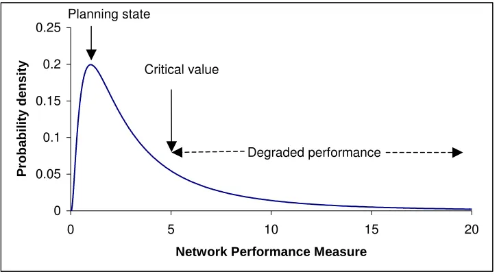
4. ILLUSTRATIVE EXAMPLE

ork will be considered, previously studied in the literature (e.g. [FIGURE 2 HERE]

A five-link test netw

Suwansirikul et al, 1987; Cho & Lo, 1999), and illustrated in Figure 2. It will later prove useful to label the routes available, with route A consisting of links 1 and 4,

route B comprising links 2 and 5, and route C comprising links 1, 3 and 5. To define

the base route choice probabilities, a probit-based SUE model is adopted, based on the

original (rather than Poisson-corrected) travel time functions, and using independent

link perception errors, distributed for link a as Nor

(

0,(φt_a(0))2

)

, with φ=0.3 used in the tests below. This SUE was estimated using 32,000 iterations of a route-based

Method of Successive Averages (MSA) algorithm, with one stochastic network load

sampled per MSA iteration. The resulting SUE link flows are provided in Table 1,

inferring route choice probabilities of pA = 0.4310, pB = 0.4452 and pC = 0.1239. [TABLE 1 HERE]

Mindful that direct use of the quartic travel time functions in the subsequent reliability

analysis could lead to a high computational cost in larger networks, a local quadratic

(second order Taylor series) approximation about the SUE solution was therefore

adopted, and the resulting error later investigated. The Taylor series coefficients (b_ia)

and the transformed coefficients (b~_ia) are also provided in Table 1.

The link flow covariance matrix (3), and thence the link-based total travel time

61,951.13

,961.

It is the

3.9755.

or comparison, these summary measures were also estimated using Monte Carlo moments (15a)−(15d), may then be estimated, whereby the total network travel time

moments about the origin can be computed as:

E[T] = 1298.39 E[T2] = 1,7

E[T3] = 2,501,598,503 E[T4] = 3,719,186,185 n straightforward to obtain the summary measures: µ = 1298.39 σ = 275.95 √β1 = 0.7696 β2 =

F

simulation, with each of 1000 pseudo-random draws of the Poisson O-D matrix

For each simulation draw, link travel times⎯and hence total network travel time⎯are

computed, using either the exact quartic functions or quadratic approximations.

[FIGURE 3 HERE]

[TABLE 2 HERE]

The empirical frequency distributions obtained from four replications of this Monte

cal moments, the algorithm of §3.3 selected a Johnson SL curve

54 δ = 4.04184 ξ = 200.067

which is rve represents a comparison with

Carlo procedure are illustrated in Figure 3. Even with as many as 1000 Monte Carlo

draws per replication (a large number for a realistic scale network), considerable

between-replication variability in the shape of the distribution may be observed. Table

2 compares the resulting summary statistics between the (exact) analytical, empirical

BPR (Monte Carlo, exact quartic functions) and empirical Taylor approximation

(Monte Carlo, approximate quadratic functions) methods. For both empirical methods

25 replications were performed, with both the mean and standard deviation across the

replications presented. Although the Monte Carlo estimates have a bias no greater

than 5%, their standard errors are as much as 15%–20% of their mean value for the

third and fourth moments. While this error may be reduced (at a computational cost)

by increasing the number of simulated draws, the potential unreliability of Monte

Carlo methods for estimating shape parameters is evident, an especially significant

factor in the study of an asymmetric/tail feature such as travel time unreliability.

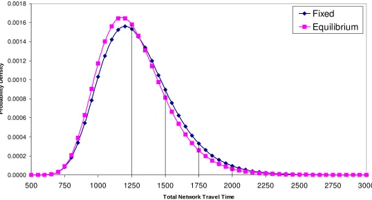
[FIGURE 4 HERE]

Based on the analyti

with parameters γ = −28.17

labelled “Fixed” in Figure 4. The second cu

the equilibrium philosophy behind most existing reliability analyses reviewed in §1,

whereby equilibrium is reached for each realisation of the system state (in this case,

the realised O-D flows). This is achieved by approximating the equilibrium response

by sensitivity analysis (Clark & Watling, 2002), obtaining equilibrium link flows

Bq d q

v*( )≈ + , with q the vector of O-D demands, d a constant A-vector and B a constant A×A matrix. As a linear model for the random O-D demand vector Q, the

link flow covariance matrix of the induced random link flows is then:

T *

] var[ ]

var[ )] (

var[v Q ≈ d+BQ =B Q B (17)

[TABLE 3 HERE]

ty probabilities’ (as

able 3, that the impact of the equilibrium response is a more

rimary method proposed in §3.1–§3.3, the impact is

onsidered of adjusting the capacity of each link in turn (base values are given in the

apacity of link 1 was gradually

to the anticipated location shift, which could be predicted by an It is clear from Figure 4, coupled with the corresponding ‘reliabili

defined in §2) in T

optimistic evaluation of reliability than the ‘fixed’ response (curve shifted to left),

whereby drivers have sufficient knowledge of prevailing conditions to mitigate the

impacts of system variation by adjusting their choice of route. Thus, we are able to

contrast the impacts of variability that is not predictable by the drivers (‘fixed’, the

primary approach of the present paper) and of predictable variation (‘equilibrium’

response), the latter perhaps more closely achievable with some kind of intelligent

driver information system.

Focusing again on the p

c

quartic term denominators of the travel time functions in Figure 2). In each case, a

new probit SUE is first computed to obtain the route choice probabilities, and a new

quadratic Taylor series approximation subsequently estimated. Figure 5 illustrates the

resultant Johnson curves, with SL(0) denoting the base case, and SL(a)/SB(a) denoting the case in which the capacity of link a alone was reduced by 10 units(a=1,2,...,5). Links 1 and 5 may be identified as the most ‘sensitive’ links, with the capacity

reductions here having the most pronounced effect.

[FIGURE 5 HERE]

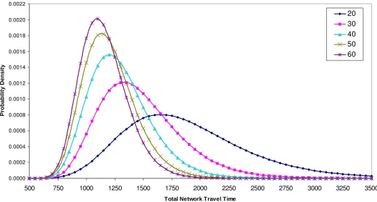
Figure 6 illustrates a further experiment, as the c

reduced. In addition

existing equilibrium model, subtle dispersion and shape impacts are also evident.

Specifically, an increase in dispersion and skewness (longer right hand tail) may be

seen, while the left-hand tail is apparently anchored. These results are plausible, in the

sense that ‘spare capacity’ allows a network to deal better with unexpected variation.

5. IMPLEMENTATION CONSIDERATIONS

s dominated by the difficulty in

omputing the highest moment, . For quadratic travel time functions (using a

o

The computational load of the method in §3 i

c E[T4]

Taylor series approximation where necessary), E[T4] will involve in the order of 4

)) 2 (

(A m+ terms requiring Isserlis m ments as high as (1,1,...,1) (see Appendix B). In §4, with A=5 and 2

12

q

=

m , around 160 q (1,1,...,1) evaluations were ich was achieved in a matter of seconds, yet clearly this will increase

rapidly with the siz the network (i.e. with A).

In large networks, an attractive simplification i

,000 ₁₂

required, wh

e of

s to restrict attention to only the

gnormal SL system, whereby only moments up to are required, the difficulty

of minutes

putational savings may be required, such as in

etworks much larger than 100 links, or as part of a method to optimise network

parameters w ts and two

lo E[T3]

then dominated by the computation of around (A(m+2))3 Isserlis moments of the )

1 ,..., 1 , 1 (

q kind. Hence both the number of terms, and the difficulty of computing each term, dramatically reduces. We have verified that practical run-times in the order

could then be achieved on current fast personal computers, for a problem

with A=100 links and m=2.

Still, there are cases where further com 8

n

reliability where multiple applications of this method are required. By assuming

structural relationships between the parameters, or fixing externally estimates of some

parameters, it is then possible that only moments up to E[T2] are required, the computational load reducing dramatically to requiring only in the order of

2 )) 2 (

(A m+ Isserlis moments of the q₆(1,1,...,1) kind. For example, in the case of SB type curves, a method is provided in Bacon-Stone (1985) to estimate all four

ith the first two momen boundary values. Prior estimates of

such boundary values might be fixed from some reasonable assumptions about the

minimum and maximum demand, or in an optimisation context from a previous full

In a similar spirit, it is straightforward to adapt the estimation of SL curves to use a

pre-specified value ₀ of the shift parameter ξ, which effectively represents the

inimum total trave e. By eliminating and from the expressions in (16)

through substitution, and setting = we obtain:

m l tim ˆ ˆ

0 ˆ

) µ ln( ˆ ˆ 2

1 ˆ µ

1 ln ˆ

2 2

0

− −

= ⎟

⎠ ⎞ ⎜

⎝ ⎛

⎟ ⎟ ⎠ ⎞ ⎜

⎜ ⎝ ⎛

⎟ ⎠ ⎞ ⎜

⎝ ⎛

− + =

−

(18)

0 1

⎟

⎜ ⎜ ⎟

whereby an SL curve may be estimated with only knowledge of and . As an

lustration, considering the moments given in Table 2 an itted c

in Figure 5, then with the full estimation of all parameters we obtain an SL curve with

a

and

µ

il d f urve denoted SL(0)

07 . 200

ˆ_{= ,} ˆ_{=4.04 and ˆ =−28.18. If, on the other hand, we m ke a very crude}

estimate of the minimum by setting ₀ = 0 and applying (18), we obtain rather similar

parameter estimates ˆ=4.77 ˆ=−34.10. In the last two columns of Table 3, the

resulting favourable comparison the reliability probabilities obtained from

),

imate Fixed’ column).

n approach has been proposed which departs in philosophy from previous analyses

element being an assumption of disequilibrium, with drivers

ssumed to face unpredictable variation to which they are not able to re-equilibrate. is given of

the full estimation (‘Fixed’ column with those from the two parameter estimation

with ₀ = 0 (‘Approx

6. CONCLUSION

A

of this topic, a key

a

Although as illustrated in §4, it is possible to implement this approach with Monte

Carlo methods, it has been shown that it is also theoretically possible to estimate

analytically moments of the network travel time probability distribution under an assumption of stochastic demand (§3.1, §3.2), from which an estimate of the full

distribution may be readily constructed (§3.3), and from which system reliability

probabilities may be computed (§2). The analytical method presented is flexible, in

that it may be tailored to the demands of the particular application: in large networks,

one can restrict the computation of moments by selecting a restricted family of

(§4) have demonstrated the application of the approach in understanding the impacts

of capacity changes on the shape of the network travel time density, beyond the effect

on mean and variance, as well as its use in identifying vulnerable or sensitive links, in

terms of their impact on overall system performance.

There are many potential avenues for further research with this technique:

1. On a practical level, a large network case-study would clearly be valuable,

including comparisons with any empirical data on variability.

advantages

bility may itself be

3.

sures under elastic (and stochastic) demand.

h

AC

e would like to thank the anonymous referees for their comments, which led us to

s.

2. In order to widen the opportunities for statistical fitting, there may be

in widening the range of underlying statistical model assumptions that are

admissible, including those in which the O-D demand varia

parameterised. One extension to the current assumptions would be to reflect

correlations in O-D demand levels due to common underlying factors.

The reliability measures themselves may be extended beyond overall network

travel time, such as O-D specific total travel time, and the day-to-day distribution

of user-average O-D travel times.

4. There are opportunities to generalise the model itself in many ways, including

extensions to reflect randomly varying link capacities, and the estimation of

reliability for economic benefit mea

5. Finally, there is potential for embedding the proposed method of reliability

evaluation within a bi-level (possibly multi-objective) optimisation framework,

whereby network capacities, tolls or information sensors may be set wit

reliability considerations in mind. The use of an analytical approach would be

expected to have particular advantages (over Monte Carlo methods), for devising

efficient gradient-based or sensitivity-analysis based algorithms in such a context.

KNOWLEDGEMENTS

W

REFERENCES

sakura Y (1996). Reliability measures of an origin and destination pair in a

d network with variable flows. In Transportation Networks: Recent Methodological Advances (ed. MGH Bell), Pergamon Press, Oxford, 273-288.

Transportation Network Reliability, Kyoto, Japan,

Ba

Bell MGH (1991). Expected equilibrium assignment under stochastic demand.

Be ent: an

Be sed approach to

Be udy of the road network in

etwork Reliability, Kyoto, Japan, July 30th – August 1st 2001. A

deteriorated roa

Asakura Y & Kashiwadani M (1991). Road network reliability caused by daily

fluctuation of traffic flow. Proceedings, 19th PTRC Summer Annual Meeting, Brighton, Seminar G, 73-84.

Asakura Y, Hato E & Kashiwadani M (2001). Stochastic Network Design Problem:

An Optimal Link Improvement Model for Reliable Network. Paper presented at 1st

International Symposium on

July 30th – August 1st 2001.

con-Shone, J (1985). Algorithm AS210. Fitting Five Parameter Johnson SB Curves

by Moments. Applied Statistics 34(1), 95-100.

Unpublished paper presented at 23rd Universities Transport Study Group Annual

Conference, Nottingham, UK, January 1991.

Bell MGH (2000). A game theory approach to measuring the performance reliability

of transport networks. Transportation Research 34B(6), 533-546.

ll MGH & Cassir C (2002). Risk-averse user equilibrium traffic assignm

application of game theory. Transportation Research36B(8), 671-682. ll MGH, Cassir C, Iida Y & Lam WHK (1999). A sensitivity-ba

network reliability assessment. In Proceedings 14th International Symposium on Transportation & Traffic Theory, Jerusalem, 283-300.

Bell MGH & Iida Y (1997). Transportation Network Analysis. John Wiley & Sons, Chichester, UK.

rdica K (2001). Vulnerability – a model-based case st

the city of Stockholm. Paper presented at 1st International Symposium on

Transportation N

Berdica K (2002). An introduction to road vulnerability: what has been done, is done

Cantarella GE & Cascetta E (1995). Dynamic processes and equilibrium in

transportation networks: Towards a unifying theory. Transportation Science 29(4), 305-329.

Chen A, Tatneni M, Lee D-H & Yang H (2000). Effect of Route Choice Models on

Estimating Network Capacity Reliability. Transportation Res Rec1733, 63-70. Chen A, Yang H, Lo HK & Tang WH (2002). Capacity reliability of a road network:

an assessment methodology and numerical results. Transportation Research

36B(3), 225-252.

Cho HJ & Lo SC (1999). Solving Bilevel Network Design Problem Using a Linear

Reaction Function Without Nondegeneracy Assumption. Transportation Research Record1667, 96-106.

Clark SD and Watling DP (2002). Sensitivity analysis of the probit-based stochastic

user equilibrium assignment problem. Transportation Research 36B(7), 617-635. D’Este GM & Taylor MAP (2001). Network vulnerability: an approach to reliability

analysis at the level of national strategic transport networks. Transport Systems

Centre, University of South Australia, Adelaide, Australia.

Davis GA & Nihan NL (1993). Large population approximations of a general

stochastic traffic assignment model. Operations Research 41(1), 169-178.

Du ZP & Nicholson AJ (1997). Degradable transportation systems: sensitivity and

reliability analysis. Transportation Research 31B(3), 225-237.

Gordon A, Van Vuren T, Watling DP, Polak J, Noland RB, Porter S & Taylor N

(2001). Incorporating variable travel time effects into route choice models. Proc PTRC European Transport Conference (Methodological Innovations), PTRC Education & Research Services Ltd., London.

Hazelton ML (1998). Some remarks on stochastic user equilibrium. Transportation Research 32B, 101-108.

Hazelton ML (2001). Inference for origin-destination matrices: estimation, prediction

and reconstruction. Transportation Research 35B(7), 667-676.

Hazelton ML & Watling DP (2003). Computing equilibrium distributions for markov

traffic assignment models. Transportation Science, in press.

Hill ID (1976). Algorithm AS100: Normal-Johnson and Johnson-Normal

Transformations. Applied Statistics 25(2), 190-192.

Hill ID, Hill R & Holder RL (1976). Algorithm AS99: Fitting Johnson Curves by

Isserlis L (1918). On a Formulation for the Product-Moment Co-efficient of any

Order of a Normal Frequency Distribution in any Number of Variables. Biometrika

12(1/2), 134-139.

Johnson NL (1949). Systems of Frequency Curves Generated by Methods of

Translation. Biometrika36(1/2), 149-176.

Karlin S & Taylor HM (1981). A second course in stochastic processes. Academic Press, London.

Liu HX, Ban X, Ran B & Mirchandani P (2002). An Analytical Dynamic Traffic

Assignment Model with Probabilistic Travel Times and Perceptions. Paper

presented at 81st annual Transportation Research Board meeting, Washington DC,

January 2002

Lo H & Tung YK (2000). A Chance Constrained Network Capacity Model. In

Reliability of Transport Networks (eds. M. Bell & C. Cassir), Research Studies Press Ltd., 159-172.

Mirchandani P & Soroush H (1987). Generalized Traffic Equilibrium with

Probabilistic Travel Times and Perceptions. Transportation Science 21(3), 133-152 Nicholson A & Du ZP (1997). Degradable transportation systems: an integrated

equilibrium model. Transportation Research 31B(3), 209-224.

Noland RB & Polak JW (2002). Travel time variability: a review of theoretical and

empirical issues. Transport Reviews22(1), 39¯54.

Noland RB, Small KA, Koskenoja PM & Chu X (1998). Simulating travel reliability.

Regional Science and Urban Economics28, 535¯564.

Sheffi Y (1985). Urban Transportation Networks.Prentice-Hall, New Jersey.

Stuart A & Ord JK (1987). Kendall’s Advanced Theory of Statistics. Volume 1: Distribution Theory. Fifth edition, Charles Griffin & Co. Ltd., London.

Suwansirikul C, Friesz TL & Tobin RL (1987). Equilibrium Decomposed

Optimization: A Heuristic for the Continuous Equilibrium Network Design

Problem. Transportation Science 21(4), 254-62

Uchida T & Iida Y (1993). Risk assignment: a new traffic assignment model

considering risk of travel time variation. In: Proc 12th International Symposium on Transportation & Traffic Theory (ed. Daganzo CF), Amsterdam, 89-105.

Watling DP (2002a). A schedule-based user equilibrium traffic assignment model.

Paper presented at 9th meeting of EURO Working Group on Transportation, Bari,

Watling DP (2002b). A second order stochastic network equilibrium model.

Transportation Science 36(2), 149-183.

Watling DP (2002c). Stochastic network equilibrium under stochastic demand. In:

Transportation Planning: State of the Art (eds. M. Patriksson & M. Labbé), Kluwer, Dordrecht, The Netherlands.

Yang H, Lo HK & Tang WH (2000). Travel time versus capacity reliability of a road

network. In Reliability of Transport Networks (eds. M. Bell & C. Cassir), Research Studies Press Ltd.

Yin Y & Ieda H (2001). Assessing performance reliability of road networks under

nonrecurrent congestion. Paper presented at 80th annual Transportation Research

Board meeting, Washington DC, January 2001.

APPENDIX A: Modified travel time functions under Poisson demand

It is reasonable to assume drivers base their decisions on long-run expected travel

times, (under (4)). Consider the case m = 2. Since under the

assumptions in §3.1, is marginally Poisson with mean (and variance)

∑

=

= m j

j a ja a

a V b V

t

0

] [ E )]

( [ E

a

V µ_a,

(

ˆ ( ),say

)

) ( ] E[ ]

[ E )]

( [

Et_a V_a =b_0a +b_1a V_a +b_2a V_a2 =t_a µ_a +b_2aµ_a =t_a µ_a

Use of the Poisson-corrected travel time function would therefore give greater

model consistency than when applied in an equilibrium framework

approximating a stochastic flow environment. The same applies for , with

higher order Poisson moments utilised (e.g.: ;

: Stuart & Ord, 1987, p 112). This refinement was first

suggested for two-link networks in an unpublished note of Bell (1991), and represents

a statistical approximation of the multinomial path flow model in Watling (2002c). (.)

ˆ

a

t

(.)

a

t

2

>

m

a a

a

V µ ) ] µ

[(

E − 3 =

) µ 3 1 ( µ ] ) µ [(

APPENDIX B: Computation of multivariate normal moments

Suppose X = is multivariate Normal with mean vector

and covariances

) ,..., ,

(X₁ X₂ X_k (µ₁,µ₂,...,µ_k)

) ,..., 2 , 1 ; ,..., 2 , 1

(i k j k

ij = = . For non-negative integers

, denote: )

,..., ,

(n₁ n₂ n_k

⎥ ⎦ ⎤ ⎢ ⎣ ⎡ − =

∏

= k i n i i k

k n n n X i

p

1 2

1, ,..., ) E ( µ )

(

and the corresponding reduced moment by

∏

= = k i n ii k k k k i n n n p n n n q 1 2 1 2 1 ) ,..., , ( ) ,..., , ( .

Now for any even positive integer m, define a pairing of order m to be a division of the set {1,2,…,m} into m_{2 subsets, each consisting of a distinct pair of elements. For}

example, if m = 6 then one possible pairing of order 6 is . In general, denote an arbitrary pairing of order m by:

}} 6 , 5 { }, 4 , 2 { }, 3 , 1 {{ ⎪⎭ ⎪ ⎬ ⎫ ⎪⎩ ⎪ ⎨ ⎧ = = = = } ,..., 3 , 2 , 1 { } { that such ,..., 2 , 1 : } , { ) , ( 2 1 ,

2 a b m

i b a m i i i m i i

U

b

a .

and denote the collection of all possible such pairings of order m by (m).

Then (Isserlis, 1918):

⎪⎩ ⎪ ⎨ ⎧ =

_{∑ ∏}

Ω ∈ = even if ~ odd if 0 ) 1 ,..., 1 , 1 ( ) ( ) , ( 1 times 2 m r m q m i b a m m m i i b a 3 2 1

where are correlation coefficients. This result can be used

to compute an arbitrary reduced moment , simply by creating an m -vector multivariate Normal where , consisting of duplicate occurrences

of each , such that

) ,..., 2 , 1 ; ,..., 2 , 1 (

~ _{i m j m}

r_ij = =

) ,..., ,

( _{1 2 k}

k n n n

q

∑

= = k i i n m 1 i n i

X ( , ,..., ) (1,1,...,1)

times 2

1 ₁₂₃

m m k

k n n n q

q = .

For example, if _⎟⎟, we would re-write:

⎠ ⎞ ⎜⎜ ⎝ ⎛ ⎟⎟ ⎠ ⎞ ⎜⎜ ⎝ ⎛ 22 12 12 11 2 1 2

1, )~Nor ( , ),

E[(X₁−µ₁)3(X₂ −µ₂)]=E[(X₁−µ₁)(X₁−µ₁)(X₁−µ₁)(X₂ −µ₂)]

with the matrix of correlation coefficients of (X₁,X₁,X₁,X₂) then:

⎟⎟ ⎟ ⎟ ⎟ ⎠ ⎞ ⎜⎜ ⎜ ⎜ ⎜ ⎝ ⎛ = ⎟⎟ ⎟ ⎟ ⎟ ⎠ ⎞ ⎜⎜ ⎜ ⎜ ⎜ ⎝ ⎛ 1 1 1 1 1 1 1 ~ ~ ~ ~ ~ ~ ~ ~ ~ ~ 12 12 12 44 34 33 24 23 22 14 13 12 11 r r r r r r r r r r r r r where 22 11 12 12 =

r .

Then by Isserlis’s result, q₄(1,1,1,1)=~r₁₂~r₃₄+~r₁₃~r₂₄+r~₁₄~r₂₃ =3r₁₂, the required reduced moment q₂(3,1) in the original system. Finally, p₂(3,1)=q₂(3,1) σ₁₁3σ₂₂ =3σ₁₂σ₁₁ . On the other hand, we would immediately know from the Isserlis result that

, since the sum of powers is 5, an odd number. 0

)] (

) [(

E X₁−µ₁ 4 X₂ −µ₂ =

The utility of the Isserlis result is particularly evident for moments involving a larger

number of variables of higher powers. In the present application, the highest order

Isserlis moment required for an nth order total travel time moment based on a kth order polynomial travel time function is n(k+1). So, for example, for a 4th order moment

based on quadratic travel time functions, we would require up to . In order

to generate such higher order Isserlis expressions, we have found a simple recursive

method to be efficient to code:

) 1 ,..., 1 , 1 ( 12 q

To determine for Y = , with m even, first denote Isserlis

reduced moments for even subsets (marginal distributions) of as: ) 1 ,..., 1 , 1 ( m

q (Y₁,Y₂,Y₃,...,Y_m)

) ,..., , ,

(Y₁ Y₂ Y₃ Y_m

) for (

1 ,..., 1 , 1 ( }) ,..., , ({ times 2

1 ₁₂₃

t t t

t i i i q

Q = ( , ,..., )

2 1 i it

i Y Y

Y 2≤t≤m, t even).

Denoting the correlation coefficients of Y by r~_ij (i=1,2,...,m; j=1,2,...,m), then for

any given m the required reduced moment (which in this new notation is ) can be generated through reduced moments of lower order,

according to the recursion: }) ,..., 3 , 2 , 1 ({ m Q_m }) , ({_{1 2}

2 i i

Q 2 1, ~ i i r = ) ,... 8 , 6 , 4 ( ) } { } ,..., , ({ ~ }) ,..., ,

({ _{2 3} c

2

2 ,

2

1 =

∑

1 ∩ =

= − t i i i i Q r i i i

Q _{t j}

where Ac denotes the complement of the set A. As a check, Isserlis (1918) provides

the explicit formula for q₆(1,1,1,1,1,1)as well as special cases of higher order moments.

a va b_0a b_1a b_2a a

b~₀ b~_1a b~_2a b~_3a

1 _{55.48 10.6637 -0.3203 0.00433 345.32 15.114 0.4005 0.00433}

2 _{44.52 10.1417 -0.2481 0.00418 328.55 12.903 0.3101 0.00418}

3 _{12.39 2.0016 -0.0004 0.00002 24.78 2.002 0.0004 0.00002}

4 43.10 8.0320 -0.1876 0.00326 258.65 10.026 0.2339 0.00326

[image:30.595.149.448.367.511.2]

5 56.90 8.5289 -0.2591 0.00342 276.50 12.263 0.3247 0.00342

Table 1: Base SUE link flows and travel time function coefficients

Analytical Empirical BPR Empirical Taylor

µ 1298.39 1265.16 (8.97) 1264.75 (7.75)

σ 275.95 271.24 (8.14) 267.14 (7.54)

√β1 0.7696 0.8303 (0.1300) 0.7882 (0.1322)

[image:30.595.113.483.571.751.2]

β2 3.9755 4.3275 (0.7485) 4.1720 (0.8330)

Table 2: Base solution total network travel time moments

Critical Value for

Total Network Travel

Time

Equilibrium Fixed

Approximate

Fixed

1250 0.4757 0.5233 0.5286

1500 0.1714 0.2108 0.2128

1750 0.0465 0.0649 0.0628

Table 3: Reliability probabilities for a number of notional critical values

[image:31.595.121.485.134.334.2]

under ‘equilibrium’ and ‘fixed’ responses (see Figure 4)

Figure 1: Illustrative example of performance measure distribution

4 1 1

1(v )=4+0.6⎜_⎝⎛v ₄₀⎟⎞_⎠

t

4

4 2 2

2(v )=6+0.9⎜_⎝⎛v ₄₀⎟⎞_⎠

t

4 3 3

3(v )= 2+0.3⎜_⎝⎛v ₆₀⎟⎞_⎠

t

5(v

[image:31.595.91.465.477.621.2]

t

O

Figure 2: Example network (Suwansirikul et al, 1987), O-D demand

4

t

4 5 5)=3+0.45⎜_⎝⎛v ₄₀⎟_⎠⎞

4 4 4) 5 0.75 ₄₀

( ⎟

⎠ ⎞ ⎜ ⎝ ⎛ +

= v

v

D

100 =

q 0

0.05 0.1 0.15 0.2 0.25

0 5 10 15 20

Network Performance Measure

P

robability density

Planning state

Critical value