This is a repository copy of A novel method for detecting the position of nonlinear components in multi-degree-of-freedom nonlinear systems.
White Rose Research Online URL for this paper: http://eprints.whiterose.ac.uk/74578/
Monograph:
Peng, Z.K., Lang, Z.Q. and Billings, S.A. (2006) A novel method for detecting the position of nonlinear components in multi-degree-of-freedom nonlinear systems. Research Report. ACSE Research Report no. 928 . Automatic Control and Systems Engineering, University of Sheffield
[email protected] https://eprints.whiterose.ac.uk/
Reuse
Unless indicated otherwise, fulltext items are protected by copyright with all rights reserved. The copyright exception in section 29 of the Copyright, Designs and Patents Act 1988 allows the making of a single copy solely for the purpose of non-commercial research or private study within the limits of fair dealing. The publisher or other rights-holder may allow further reproduction and re-use of this version - refer to the White Rose Research Online record for this item. Where records identify the publisher as the copyright holder, users can verify any specific terms of use on the publisher’s website.
Takedown
If you consider content in White Rose Research Online to be in breach of UK law, please notify us by
A Novel Method for Detecting the Position of
Nonlinear Components in
Multi-Degree-of-Freedom Nonlinear Systems
Z K Peng, Z Q Lang, and S A Billings
Department of Automatic Control and Systems Engineering The University of Sheffield
Mappin Street, Sheffield S1 3JD, UK
A Novel Method for Detecting the Position of
Nonlinear Components in
Multi-Degree-of-Freedom Nonlinear Systems
Z.K. Peng, Z.Q. Lang, and S. A. Billings
Department of Automatic Control and Systems Engineering, University of Sheffield Mappin Street, Sheffield, S1 3JD, UK
Email: [email protected]; [email protected]; [email protected]
Abstract: Based on the Nonlinear Output Frequency Response Functions (NOFRFs), a novel method is developed to detect the position of nonlinear components in MDOF nonlinear systems. The validity of this method is demonstrated by numerical studies. Although the method assumes that the linear stiffness and damping for MDOF systems under study are known a priori, the results of the numerical studies indicate that, even if only approximate values of the linear stiffness and damping parameters are used, the method can still correctly detect the position of the nonlinear component. Since the position of a nonlinear component often corresponds to the location of a defect in a MDOF system, this new method is of practical great significance for fault diagnosis in mechanical and structural systems.
1 Introduction
In engineering practice, for many mechanical and structural systems, more than one set of coordinates are needed to describe the system behaviors. This implies an MDOF model is needed to describe the system. In addition, there are considerable mechanical and structural MDOF systems that behave nonlinearly just because one or a few components have nonlinear properties. One of the well known examples is beam structures [1] with breathing cracks, the global nonlinear behaviors of which are caused only by a few cracked elements. These nonlinear MDOF systems are locally nonlinear MDOF systems where the nonlinear component is often the component where a fault or abnormal condition occurs. Therefore it is of great significance to effectively detect the position of the nonlinear component in a MDOF system.
a series of multi-dimensional convolution integrals. The Fourier transforms of the Volterra kernels are known as the kernel transforms, Higher-order Frequency Response Functions (HFRFs) [3], or more usually Generalised Frequency Response Functions (GFRFs). These provide a convenient concept for analyzing nonlinear systems in the frequency domain. If a differential equation or discrete-time model is available for a nonlinear system, the GFRFs can be determined using the algorithm in [4]~[6]. The GFRFs can be regarded as the extension of the classical frequency response function (FRF) for linear systems to the nonlinear case. The concept of Nonlinear Output Frequency Response Functions (NOFRFs) [7] is an alternative extension of the FRF to the nonlinear case. NOFRFs are one dimensional functions of frequency, which allow the analysis of nonlinear systems to be implemented in a manner similar to the analysis of linear systems, and which provides great insight into the mechanisms which dominate many important nonlinear behaviors.
In this paper, a novel quick method is derived based on the NOFRF concept to detect the position of the nonlinear component in a MDOF nonlinear system under the assumption that the values of the linear stiffness and damping for the MDOF nonlinear system are known a priori. Numerical studies verify the effectiveness of the method and indicate that, even if only the approximate values of the linear stiffness and damping parameters are used, the method can still correctly detect the position of the nonlinear component. The new method is of practical great significance for fault diagnosis in mechanical and structural systems.
The paper is organized as follows. Section 2 gives a brief introduction to the new concept of NOFRFs. Some important properties of the NOFRFs for locally nonlinear MDOF systems, which were first revealed in the authors’ recent studies [8], are introduced in Section 3. The novel method for the nonlinear component position detection is presented in Section 4. In Section 5, two numerical case studies are used to verify the effectiveness of the proposed method. Finally conclusions are given in Section 6.
2. Output Frequency Response Functions of Nonlinear Systems
2.1 Output Frequency Response Functions under General Input
Consider the class of nonlinear systems which are stable at zero equilibrium and which can be described in the neighbourhood of the equilibrium by the Volterra series
i n
i
i n
N n
n u t d
h t
y( ) (τ ,...,τ ) ( τ ) τ
1 1
1
∏
∑∫ ∫
= =
∞ ∞ −
∞ ∞
− −
= L (1)
where y(t) and u(t) are the output and input of the system, hn(τ1,...,τn) is the nth order Volterra kernel, and N denotes the maximum order of the system nonlinearity. Lang and Billings [3] derived an expression for the output frequency response of this class of nonlinear systems to a general input. The result is
⎪ ⎪ ⎩ ⎪ ⎪ ⎨ ⎧
=
∀ =
∫
∏
∑
= +
+ =
− =
ω ω ω
ω
σ ω ω
ω π
ω
ω ω
ω
n 1
n n
1 i
i n
1 n 1
n n
N 1 n
n
d j U j
j H 2
n 1 j
Y
j Y j
Y
,...,
) ( ) ,..., ( )
( ) (
for
) ( )
(
(2)
This expression reveals how nonlinear mechanisms operate on the input spectra to produce the system output frequency response. In (2), Y(jω) is the spectrum of the system output, Yn(jω) represents the nth order output frequency response of the system,
n j
n n
n
n j j h e d d
H ( ω ,..., ω ) ... (τ ,...,τ ) ωτ ωnτn τ ... τ
1 ) ,..., ( 1
1
1 1 + +
− ∞
∞ − ∞
∞
−
∫
∫
= (3)
is the nth order Generalised Frequency Response Function (GFRF) [3], and
∫
∏
= +
+ ω ω =
ω
ω
σ ω ω
ω n
n n
i
i n
n j j U j d
H
,..., 1
1
1
) ( ) ,..., (
denotes the integration of
∏
over the n-dimensional hyper-plane =n i
i n
n j j U j
H
1
1,..., ) ( )
( ω ω ω
ω ω
ω1+L+ n = . Equation (2) is a natural extension of the well-known linear relationship )
( ) ( )
(jω H jωU jω
Y = , where H(jω) is the frequency response function, to the nonlinear case.
For linear systems, the possible output frequencies are the same as the frequencies in the input. For nonlinear systems described by equation (1), however, the relationship between the input and output frequencies is more complicated. Given the frequency range of an input, the output frequencies of system (1) can be determined using the explicit expression derived by Lang and Billings in [3].
∫ ∏
∫
∏
= +
+ =
= +
+ =
=
ω ω ω
ω ω
ω ω
ω
σ ω
σ ω ω
ω ω
n n
n n
i
i
n n
i
i n
n
n
d j U
d j U j
j H
j G
,..., 1
,..., 1
1
1 1
) (
) ( ) ,..., (
)
( (4)
under the condition that
0 )
( )
(
,..., 1
1
≠
=
∫ ∏
= +
+ ω ω =
ω
ω
σ ω ω
n
n n
i
i
n j U j d
U (5) Notice that Gn(jω) is valid over the frequency range of Un(jω) , which can be determined using the algorithm in [3].
By introducing the NOFRFs Gn(jω), n=1,LN, equation (2) can be written as
∑
∑
= =
=
= N
n
n n
N n
n j G j U j
Y j
Y
1 1
) ( ) ( )
( )
( ω ω ω ω (6) which is similar to the description of the output frequency response for linear systems. The NOFRFs reflect a combined contribution of the system and the input to the system output frequency response behaviour. It can be seen from equation (4) that Gn(jω) depends not only on Hn (n=1,…,N) but also on the input U(jω). For any structure, the dynamical properties are determined by the GFRFs (n= 1,…,N). However, from equation (3) it can be seen that the GFRF is multidimensional [9][10], which can make the GFRFs difficult to measure, display and interpret in practice. Feijoo, Worden and Stanway [11][12] demonstrated that the Volterra series can be described by a series of associated linear equations (ALEs) whose corresponding associated frequency response functions (AFRFs) are easier to analyze and interpret than the GFRFs. According to equation (4), the NOFRF
n H
) (jω
Gn is a weighted sum of Hn(jω1,..., jωn) over ω
ω
ω1+L+ n = with the weights depending on the test input. Therefore Gn(jω) can be used as an alternative representation of the dynamical properties described by . The most important property of the NOFRF
n H )
(jω
Gn is that it is one dimensional, and thus allows the analysis of nonlinear systems to be implemented in a convenient manner similar to the analysis of linear systems. Moreover, there is an effective algorithm [7] available which allows the estimation of the NOFRFs to be implemented directly using system input output data.
2.2 Output Frequency Response Functions under Harmonic Inputs
When system (1) is subject to a harmonic input ) cos(
)
(t = A ω t+β
u F (7) Lang and Billings [3] showed that equation (2) can be expressed as
∑
∑
∑
= + + = = ⎟ ⎟ ⎠ ⎞ ⎜ ⎜ ⎝ ⎛ = = N n k k k k n n N n n kn k nn A j A j
j j H j Y j Y 1 1 1 1
1, , ) ( ) ( )
( 2 1 ) ( ) ( ω ω ω ω ω ω ω ω ω L L
L (8)
where ⎩ ⎨ ⎧ = 0 | | ) ( ) ( sign β ωk A ej k j
A
i
if
{
}
otherwise , , 1 , 1
,k i n
k F
ki ∈ ω =± = L
ω
(9) Define the frequency components of nth order output of the system as . Then according to equation (8), the frequency components in the system output can be expressed as n Ω
U
N n n 1 = Ω =Ω (10) and Ωn is determined by the set of frequencies
{
k k k F i n}
i
n | , 1, ,
1+L+ =± = L
=ω ω ω ω
ω (11) From equation (11), it is known that if all
n
k
k ω
ω , ,
1 L are taken as −ωF, then ω=−nωF.
If k of these are taken as ωF, then ω =(−n+2k)ωF. The maximal k is n. Therefore the possible frequency components of Yn(jω) are
n
Ω =
{
(−n+2k)ωF,k =0,1,L,n}
(12) Moreover, it is easy to deduce that} , , 1 , 0 , 1 , , , { 1 N N k k F N n
n L L
U
Ω = =− −= Ω
=
ω (13) Equation (13) explains why superharmonic components are generated when a nonlinear system is subjected to a harmonic excitation. In the following, only those components with positive frequencies will be considered.
The NOFRFs defined in equation (4) can be extended to the case of harmonic inputs as
∑
∑
= + + = + + = ω ω ω ω ω ω ω ω ω ω ω ω ω kn k n kn k n n k k n k k k k n n H n j A j A j A j A j j H j G L L L L L 1 1 1 1 1 ) ( ) ( 2 1 ) ( ) ( ) , , ( 2 1 )( n = 1,…, N (14)
under the condition that
0 ) ( ) ( 2 1 ) ( 1 1 ≠ =
∑
= ++ ω ω
ω ω ω ω kn k n k k n
n j A j A j
A
L
Obviously, is only valid over GnH(jω) Ωn defined by equation (12). Consequently, the output spectrum Y(jω) of nonlinear systems under a harmonic input can be expressed as
∑
∑
= =
=
= N
n
n H
n N
n
n j G j A j
Y j
Y
1 1
) ( ) ( )
( )
( ω ω ω ω (16) When k of the n frequencies of
n
k
k ω
ω , ,
1 L are taken as ωF and the remainders are as
F ω
− , substituting equation (9) into equation (15) yields,
β
ω ( 2 )
| | 2
1 ) ) 2 (
( F n n j n k
n j n k A e
A − + = − + (17) Thus becomes GnH(jω)
β
β
ω ω
ω ω
ω
) 2 (
) 2 (
| | 2
1
| | ) , , ,
, , ( 2
1 ) ) 2 ( (
k n j n n
k n j n k
n
F F
k F F
n n F H
n
e A
e A j
j j
j H k
n j G
+ −
+ − −
− −
= +
−
4 4 8 4
4 7 6
L 4
48 4
47 6
L
) , , ,
, , (
4 4 8 4
4 7 6
L 4
48 4 47 6
L
k n
F F
k F F
n j j j j
H
−
− −
= ω ω ω ω (18) where Hn(jω1,...,jωn) is assumed to be a symmetric function. Therefore, in this case,
over the nth order output frequency range )
(jω
GnH Ωn=
{
(−n+2k)ωF,k =0,1,L,n}
is equal to the GFRFHn(jω1,...,jωn) evaluated atω1 =L=ωk =ωF, ωk+1 =L=ωn =−ωF,. n k=0,L,
3. NOFRFs of Locally Nonlinear MDOF Systems
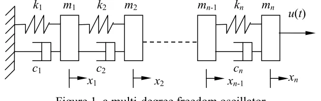
[image:8.612.148.464.468.568.2]The locally nonlinear MDOF systems to be investigated are as shown in Figure 1.
Figure 1, a multi-degree freedom oscillator
If all springs and damper are of linear properties, then the governing motion equation of the MDOF oscillator in Figure 1 can be written as
) (t U Kx x C x
M&&+ &+ = (19) where M is the system mass matrix,
where
kn mn
k1 m1 k2 m2 mn-1
u(t)
x1 x2 xn-1 xn
cn
c2
⎥ ⎥ ⎥ ⎥ ⎦ ⎤ ⎢ ⎢ ⎢ ⎢ ⎣ ⎡ = n m m m M L M O M M L L 0 0 0 0 0 0 2 1
is the system mass matrix, and
⎥ ⎥ ⎥ ⎥ ⎥ ⎥ ⎦ ⎤ ⎢ ⎢ ⎢ ⎢ ⎢ ⎢ ⎣ ⎡ − − + − − + − − + = − − n n n n n n c c c c c c c c c c c c c C 0 0 0 0 0 0 1 1 3 3 2 2 2 2 1 L O M O O O M O L ⎥ ⎥ ⎥ ⎥ ⎥ ⎥ ⎦ ⎤ ⎢ ⎢ ⎢ ⎢ ⎢ ⎢ ⎣ ⎡ − − + − − + − − + = − − n n n n n n k k k k k k k k k k k k k K 0 0 0 0 0 0 1 1 3 3 2 2 2 2 1 L O M O O O M O L
are the system damping and stiffness matrix respectively. is the displacement vector, and
' 1, , ) (x xn x= L
' 1 ) 0 , , 0 ), ( , 0 , , 0 ( ) ( 8 7 6 L 8 7 6 L J n J t f t F − − =
is the external force vector acting on the oscillator.
Equation (19) is the basis of the modal analysis method, which is a well-established approach for determining dynamic characteristics of engineering structures. In the linear case, the displacements xi(t) (i=1,L,n) can be expressed as
∫
−+∞∞ −= h t τ f τ dτ t
xi( ) (i)( ) ( ) (20) where ( ) are the impulse response functions that are determined by equation (19), and the Fourier transform of is the well-known FRF.
) ( ) ( t
hi i=1,L,n
) ( ) ( t hi
Assume the Lth spring has nonlinear stiffness and damping, and the restoring forces and are the polynomial functions of the deformation and )
(∆ LS
S SLD(∆&) ∆& respectively, e.g.,
∑
= ∆ = ∆ P i i i LS r S 1 )( ,
∑
(21) = ∆ = ∆ P i i i LD w S 1 )(& &
where P is the degree of the polynomial. Without loss of generality, further assume . Then the motion of the oscillator in Figure 3 is determined by equations (22)~(26) as follows.
n L≠1,
For the masses that are not connected to the Lth spring, the governing motion equations are 0
) (
)
( 1 2 1 2 2 1 2 1 2 2
1
1x + c +c x −c x + k +k x −k x =
m&& & & (22) 0
) (
)
( + 1 − 1− 1 1+ + 1 − 1− 1 1 =
+ i i+ i i i− i+ i+ i i+ i i i− i+ i+
i
ix c c x cx c x k k x k x k x m&& & & &
(i≠L−1,L) (23) 0
1
1+ − =
−
+ n n n n− n n n n−
n
nx c x c x k x k x
m && & & (24) Denote and , then for the mass that is connected to the left of the Lth spring, the governing motion equation is
1 r
0 ) ( ) ( ) ( ) ( 2 1 2 1 2 1 1 1 2 1 1 1 1 1 = − + − + − − + + − − + +
∑
∑
= − = − − − − − − − − − − − P i i L L i P i i L L i L L L L L L L L L L L L L L L L x x w x x r x c x c x c c x k x k x k k x m & & & & & & & (25)For the mass that is connected to the right of the Lth spring, the governing motion equation is 0 ) ( ) ( ) ( ) ( 2 1 2 1 1 1 1 1 1 1 1 1 = − − − − − − + + − − + +
∑
∑
= − = − + + − + + + − + P i i L L i P i i L L i L L L L L L L L L L L L L L L L x x w x x r x c x c x c c x k x k x k k x m & & & & & & & (26) Denote∑
∑
= − = − − + − = P i i L L i P i i L Li x x r x x
w NonF
2 1 2
1 ) ( )
(& & (27)
(
)
'0 0
0
0 L NonF NonF L
NF = − (28) Then, equation (22)~(26) can be rewritten in a matrix form as
) (t F NF Kx x C x
M&&+ &+ =− + (29) The system described by equations (27)~(29) is a typical locally nonlinear MDOF system. The Lth nonlinear component can lead the whole system to behave nonlinearly. In this case, the Volterra series can be used to describe the relationships between the displacements (xi(t) i=1,L,n) and the input force f(t) as below
(30) i j i i N j j j i
i t h f t d
x ( ) (τ ,...,τ ) ( τ ) τ 1 1 1 ) , (
∏
∑∫ ∫
= = ∞ ∞ − ∞ ∞ − − = Lwhere h(i,j)(τ1,...,τj) is the jth order Volterra kernel associated to the ith mass. In the frequency domain, the relationship (30) can be expressed as
∑
∑
= = = = N l l l i N l l ii j X j G j U j
X 1 ) , ( 1 ) , ( ( ) ( ) ( ) )
( ω ω ω ω (i=1,L,n) (31) where )G(i,l)(jω is the lth order NOFRF associated to the ith mass.
As the authors’ recent studies [8] revealed, for any two consecutive masses, the NOFRFs satisfy ) ( ) ( ) ( ) ( ) ( ) ( ) , 1 ( ) , ( 1 , ) 2 , 1 ( ) 2 , ( 1 , 2 ω ω ω λ ω ω ω λ j G j G j j G j G j N i N i i i N i i i i + + +
+ = =L= =
(1≤i≤n−1) (32) and ) ( ) ( ) ( ) ( ) ( )
( , 1
) , 1 ( ) , ( ) 1 , 1 ( ) 1 , ( 1 ,
1 ω λ ω
ω ω ω ω λ j j G j G j G j G
j ii
Z Z i Z i i i i i + + + + = = =
(1≤i≤L−2,2≤Z ≤N) (33) and ) ( ) ( ) ( ) ( ) ( )
( , 1
) , 1 ( ) , ( ) 1 , 1 ( ) 1 , ( 1 ,
1 ω λ ω
ω ω ω ω λ j j G j G j G j G
j iZi
Z i Z i i i i i + + + + = ≠ =
(
)
(
)
[
− + − + + + +]
⎜⎜⎝⎛ + Λ + ⎞⎠⎟⎟= + + + + + − + + + 1 1 1 , 1 1 , 1 2 1 1 1 , ( ) 1 ) ( 1 ) ( i i i i Z i i i i i i Z i i i i i Z k jc j k jc k jc j m k jc j ω ω ω ω ω λ ω ω ω λ
(1≤i≤n−1,1≤Z ≤N ) (35) and ⎪ ⎪ ⎪ ⎪ ⎩ ⎪⎪ ⎪ ⎪ ⎨ ⎧ = ≥ Γ − = ≥ Γ − − ≠ = = Λ + − − + and 2 for ) ( ) ( 1 and 2 for ) ( ) ( , 1 or 1, for 0 ) ( ) , 1 ( ) , 1 ( ) , ( ) , 1 ( 1 , L i Z j G j L i Z j G j L L i Z j Z L Z L Z L Z L i i Z ω ω ω ω
ω (36)
and Γ(L−1,Z)(jω) is a term introduced by the nonlinear force NonF for the Zth order NOFRF.
Furthermore, λiZ,i+1(jω) (2≤Z ≤N) can also be described as [8] ) ( ) ( ) ( ) ( ) ( , 1 1 , 1 , 1 , 1 , ω ω ω ω ω λ j Q j Q j Q j Q j L i L i L i L i i i Z + − + − + − −
= (i=1,L,n−1) (37) where
(
2)
1) , ( ) 1 , ( ) , 1 ( ) 1 , 1 ( ) ( ) ( ) ( ) ( − + + − = ⎟ ⎟ ⎟ ⎠ ⎞ ⎜ ⎜ ⎜ ⎝ ⎛ K jC M j Q j Q j Q j Q n n n n ω ω ω ω ω ω L M O M L (38)
When the input u(t) is a sinusoidal type force of frequency ωF , according to the definition of NOFRFs under a harmonic input in Section 2.2, it is known from equation (32), that ) 2 ( ) ( ) ( ) 2 ( ) 2 ( ) 2 ( ) 2
( , 1
) 2 , 1 ( ) 2 , ( ) 4 , 1 ( ) 4 , ( ) 2 , 1 ( ) 2 , ( F i i J i J i F i F i F i F i j j G j G j G j G j G j G ω λ ω ω ω ω ω ω + + + + = = = =
= L L
) 3 ( ) 3 ( ) 3 ( ) 3 ( ) 3 ( ) 3 ( ) 3
( , 1
) 1 2 , 1 ( ) 1 2 , ( ) 5 , 1 ( ) 5 , ( ) 3 , 1 ( ) 3 , ( F i i F J i F J i F i F i F i F i j j G j G j G j G j G j G ω λ ω ω ω ω ω ω + + + + + + = = = =
= L L
M (J =1,2,L) (i=1,L,n−1) (39) Moreover, according to equations (16) and (17), the 2nd order superharmonic component of (xi(t) i=1,L,n) can be written as
) 2 ( ) 2 ( ) 2 ( ) 2 ( ) 2 ( ) 2 ( ) 2 ( ) 2 ( 1 1 , 0 2 2 ) 2 2 , 1 ( 1 , 0 2 2 ) 2 2 , ( F i F i i J F J F J i F i i J F J F J i F i j X j j A j G j j A j G j X ω ω λ ω ω ω λ ω ω ω + + = + + + + = + + = = =
∑
∑
) 1 , , 1(i= L n− (40) Consequently ) 2 ( ) 2 ( ) 2 ( 1 1 , F i F i F i i j X j X j ω ω ω λ + + =
Similarly, it can be deduced that
) (
) (
) (
1 1
,
F i
F i F
i i
jD X
jD X jD
ω ω ω
λ
+
+ =
(D≥2,i=1,L,n−1) (42) Equation (42) provides a simple way to estimate the for a locally nonlinear MDOF system subjected to a harmonic excitation. Based on equations (37), (38) and (42), a novel method for detection of the position of the nonlinear component in MDOF nonlinear systems can be developed.
) ( 1 ,
F i
i
jDω λ +
4. A Novel Method for the Nonlinear Component Position
Detection
Assume the system masses, linear stiffness, and damping are known a priori. Then from equations (37) and (38), the theoretical λi,i+1(jω)=λiZ,i+1(jω),(Z ≥2, ) can be determined at any frequency of interest. It is known from (37) that , ( 1) are different if the nonlinear element is at a different position in a MDOF system, and there are in total n different sets of , (
1 , ,
1 −
= n
i L
) ( 1
, ω
λii+ j ,
,
1 −
= n
i L
) ( 1
, ω
λii+ j i=1,L,n−1) which correspond to the nonlinear element is located in front of mass 1, in front of mass 2,…, and in front of mass n, respectively. Therefore, λi,i+1(jω), (i=1,L,n−1) can more comprehensively be denoted as λi,i+1(jω,P) , ( i=1,L,n−1 , ) with
( 1) representing the case where the nonlinear element is in front of mass P.
n P=1,L, )
, ( 1 ,
P j i
i ω
λ +
, ,
1 −
= n
i L
When using a sinusoidal force to excite the system (29), from the FFT spectra of all masses, the values of λi,i+1(jDωF) (D≥2,i=1,L,n−1) can be estimated using equation (42). Denote the estimated λi,i+1(jDωF) as λˆi,i+1(jDωF), (i=1,L,n−1). The estimated
, ( ,
) (
ˆ, 1 F i
i
jDω λ +
2
≥
D i=1,L,n−1), reflect the real situation regarding the MDOF system under investigation, and if there exists a nonlinear element in front of mass P* in the system, then λˆi,i+1(jDωF), (D≥2, i=1,L,n−1) be very close to
( 1 ) where
) , ( 1 ,
P jD F i
i ω
λ + ,
,
1 −
= n
i L P*∈
{
1,L,n}
. Consequently, comparing( ) with ,(
) (
ˆ, 1 F i
i
jDω λ + 1
, ,
1 −
= n
i L λi,i+1(jDωF,P) i=1,L,n−1) for P=1,L,n respectively, the position of the nonlinear component in the system can be detected. This procedure can be finished using only one super-harmonic component. To compare the theoretical and estimated , the following criterion is defined. λi,i+1(jDωF)
∑
− =+
+ −
= 1
1
1 , 1
,
) (
ˆ ) , ( )
, (
n i
F i
i F
i i
F P jD P jD
D
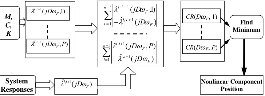
( , ). Therefore it is readily apparent when there is no need to use the above detection procedure. The novel nonlinear component position detection method can be illustrated as Figure 2. This method requires only once testing on the system excited by a sinusoidal force, and this testing is very easy to carry out in practices. In the following section, the validation of this method will be demonstrated using numerical studies.
2
≥
[image:13.612.94.525.179.336.2]D i=1,L,n−1
Figure 2, An illustration of the nonlinear component position detection method
4 Numerical Studies
In order to verify the nonlinear component position detection method, a damped 6-DOF oscillator was used, in which the fourth spring was nonlinear. The damping was assumed to be a proportional damping, e.g., C=µK in the system.
Case Study 1:
In this case study, it was assumed that exact values of the system parameters were known, such that
1 6 1 = =m =
m L , r1=k1 =k2 =k3 =3.6×10⁴, k4 =k5 =k6 =0.8k1, 01
. 0
=
µ , r2 =0.8×r12, r3 =0.4×r13, w1 =µr1, w2 =0
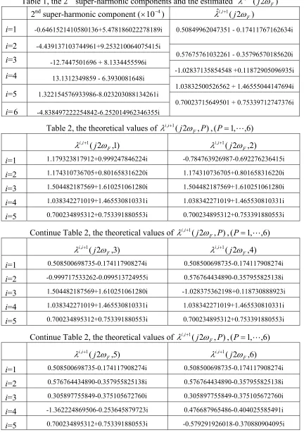
A sinusoidal force f(t)=sin(2π×20t) was imposed at the right end of this system. The responses of the system were obtained using a fourth-order Runge–Kutta method. The second super-harmonic components were used to evaluated , which were extracted from the FFT spectra of the time domain responses of the system for all masses. The results of the second super-harmonic components are given in Table 1 together with the estimated values of (i=1,2,3,4,5).
) 2 ( ˆ, 1
F i
i
j ω λ +
) 2 ( ˆ, 1
F i
i
j ω λ +
M, C, K
) 1 , (
1 ,
F i
i
jDω
λ +
) , (
1 ,
P jD F
i
i ω
λ +
System
Responses ( )
ˆ, 1 F i
i
jDω
λ +
∑
−= +
+
−
1
1 , 1 1 ,
) ( ˆ
) , ( n
i ii F
F i
i
jD P jD
ω λ
ω λ
∑
−= +
+
−
1
1 , 1 1 ,
) ( ˆ
) 1 , ( n
i F
i i
F i
i
jD jD
ω λ
ω λ
CR(D F, 1)
Find Minimum
CR(D F, P)
Table 1, the 2nd super-harmonic components and the estimated λi,i+1(j2ωF) 2nd super-harmonic component (×10−4) λˆi,i+1(j2ωF)
i=1 -0.6461521410580136+5.478186022278189i 0.50849962047351 - 0.17411767162634i
i=2 -4.439137103744961+9.253210064075415i
0.57675761032261 - 0.35796570185620i
i=3 -12.7447501696 + 8.1334455596i
-1.02837135854548 +0.11872905096935i
i=4 13.1312349859 - 6.3930081648i
1.03832500526562 + 1.46555044147694i
i=5 1.322154576933986-8.023203088134261i
i=6 -4.838497222254842-6.252014962346355i
0.70023715649501 + 0.75339712747376i
Table 2, the theoretical values of λi,i+1(j2ωF,P),(P=1,L,6) )
1 , 2 ( 1 ,
F i
i
j ω λ +
) 2 , 2 ( 1 ,
F i
i
j ω λ +
i=1 1.179323817912+0.999247846224i -0.784763926987-0.692276236415i
i=2 1.174310736705+0.801658316220i 1.174310736705+0.801658316220i
i=3 1.504482187569+1.610251061280i 1.504482187569+1.610251061280i i=4 1.038342271019+1.465530810331i 1.038342271019+1.465530810331i i=5 0.700234895312+0.753391880553i 0.700234895312+0.753391880553i
Continue Table 2, the theoretical values of λi,i+1(j2ωF,P), ) )
6 , , 1 (P= L
) 3 , 2 ( 1 ,
F i
i j ω λ +
4 , 2 ( 1 ,
F i
i j ω λ +
i=1 0.508500698735-0.174117908274i 0.508500698735-0.174117908274i i=2 -0.999717533262-0.099513724955i 0.576764434890-0.357955825138i
i=3 1.504482187569+1.610251061280i -1.028375362198+0.118730888923i
i=4 1.038342271019+1.465530810331i 1.038342271019+1.465530810331i i=5 0.700234895312+0.753391880553i 0.700234895312+0.753391880553i
Continue Table 2, the theoretical values of λi,i+1(j2ωF,P), ) )
6 , , 1 (P= L
) 5 , 2 ( 1 ,
F i
i
j ω λ +
6 , 2 ( 1 ,
F i
i
j ω λ +
i=1 0.508500698735-0.174117908274i 0.508500698735-0.174117908274i
i=2 0.576764434890-0.357955825138i 0.576764434890-0.357955825138i i=3 0.305897755849-0.375105672760i 0.305897755849-0.375105672760i
i=4 -1.362224869506-0.253645879723i 0.476687965486-0.404025585491i
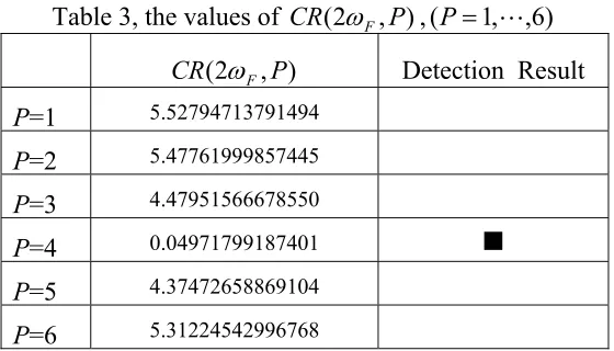
Table 3, the values of CR(2ωF,P),(P=1,L,6) )
, 2
( P
CR ωF Detection Result
P=1 5.52794713791494
P=2 5.47761999857445
P=3 4.47951566678550
P=4 0.04971799187401
P=5 4.37472658869104
P=6 5.31224542996768
The theoretical results of λi,i+1(j2ωF,P),(P=1,L,6)calculated by equations (37) and (38) are given in Table 2. The results of CR(2ωF,P),(P=1,L,6) are given in Table 3. Obviously, when P=4, CR(2ωF,P) reaches a minimum, therefore P*=4 and the nonlinear component is located in front of the fourth mass of the MDOF nonlinear system.
Case Study 2:
In this case study, was is assumed that the true values of the system parameters are the same as those used in Case Study 1, but the following approximate linear parameters were used in the computations for the method
1 6 1 = =m = m L ,
, 10 6 . 3 1 .
1 4
2
1 =k = × ×
k k3 =k4 =k6 =0.9×3.6×104, ,
10 6 . 3 7 .
0 4
5 = × ×
k µ=0.01
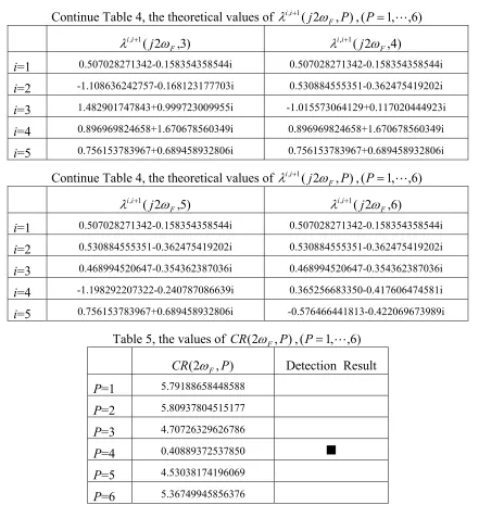
Using the above parameters, λi,i+1(j2ωF,P),(P=1,L,6) can be calculated by equations (37) and (38), and the results are given in Table 4. Obviously, the values of
estimated from the output responses are the same as the results in Table 1.
) 2 ( ˆ, 1
F i
i
j ω λ +
Table 4, the theoretical values of λi,i+1(jωF,P),(P=1,L,6) )
1 , 2 ( 1 ,
F i
i
j ω λ +
) 2 , 2 ( 1 ,
F i
i
j ω λ +
i=1 1.253371165233+0.887250572073i -0.736586166221-0.594551469301i
i=2 1.168186285650+1.020346052706i 1.168186285650+1.020346052706i
[image:15.612.96.520.508.648.2]Continue Table 4, the theoretical values of λi,i+1(j2ωF,P),(P=1,L,6) )
3 , 2 ( 1 ,
F i
i
j ω λ +
) 4 , 2 ( 1 ,
F i
i
j ω λ +
i=1 0.507028271342-0.158354358544i 0.507028271342-0.158354358544i
i=2 -1.108636242757-0.168123177703i 0.530884555351-0.362475419202i i=3 1.482901747843+0.999723009955i -1.015573064129+0.117020444923i i=4 0.896969824658+1.670678560349i 0.896969824658+1.670678560349i
i=5 0.756153783967+0.689458932806i 0.756153783967+0.689458932806i
Continue Table 4, the theoretical values of , 1(j2 ,P), F
i
i ω
λ +
) 6 , , 1 (P= L
) 5 , 2 ( 1 ,
F i
i
j ω λ +
) 6 , 2 ( 1 ,
F i
i
j ω λ +
i=1 0.507028271342-0.158354358544i 0.507028271342-0.158354358544i
i=2 0.530884555351-0.362475419202i 0.530884555351-0.362475419202i
i=3 0.468994520647-0.354362387036i 0.468994520647-0.354362387036i
[image:16.612.87.528.67.532.2]i=4 -1.198292207322-0.240787086639i 0.365256683350-0.417606474581i i=5 0.756153783967+0.689458932806i -0.576466441813-0.422069673989i
Table 5, the values of CR(2ωF,P),(P=1,L,6) )
, 2
( P
CR ωF Detection Result
P=1 5.79188658448588
P=2 5.80937804515177
P=3 4.70726329626786
P=4 0.40889372537850
P=5 4.53038174196069
P=6 5.36749945856376
The results of CR(2ωF,P),(P=1,L,6) are given in Table 4. Obviously, when P=4, )
, 2
( P
CR ωF reaches a minimum, therefore again the nonlinear component is determined to be in front of the fourth mass of the MDOF nonlinear system. This case study implies that, even if the exact information of the system is not available, the nonlinear component position method can still achieve a good result.
5 Conclusions and Remarks
damping parameters are assumed to be known a priori. Two numerical studies have been used to demonstrate the effectiveness of this method. The results show that, even if only approximate values of the linear stiffness and damping parameters are available, the method can still achieve a correct detection of the position of the nonlinear component. The distinct advantage of this method is that it only needs a set of test data under a sinusoidal input force. Since the position of the nonlinear component in a MDOF system often corresponds to the location of a fault, the nonlinear component position detection method is of practical significance for the fault diagnosis in mechanical and structural systems.
Acknowledgements
The authors gratefully acknowledge the support of the Engineering and Physical Science Research Council, UK, for this work.
References
1. T.G. Chondros, A.D. Dimarogonas, J. Yao, Vibration of a beam with breathing crack, Journal of Sound and Vibration, 239 (2001) 57-67
2. K. Worden, G. Manson, G.R. Tomlinson, A harmonic probing algorithm for the multi-input Volterra series. Journal of Sound and Vibration201(1997) 67-84 3. Z. Q. Lang, S. A. Billings, Output frequency characteristics of nonlinear system,
International Journal of Control 64 (1996) 1049-1067.
4. S.A. Billings, K.M. Tsang, Spectral analysis for nonlinear system, part I: parametric non-linear spectral analysis. Mechanical Systems and Signal Processing, 3 (1989) 319-339
5. S.A. Billings, J.C. Peyton Jones, Mapping nonlinear integro-differential equations into the frequency domain, International Journal of Control 52(1990) 863-879. 6. J.C. Peyton Jones, S.A. Billings, A recursive algorithm for the computing the
frequency response of a class of nonlinear difference equation models. International Journal of Control50 (1989) 1925-1940.
7. Z. Q. Lang, S. A. Billings, Energy transfer properties of nonlinear systems in the frequency domain, International Journal of Control78 (2005) 354-362.
9. H. Zhang, S. A. Billings, Analysing non-linear systems in the frequency domain, I: the transfer function, Mechanical Systems and Signal Processing7 (1993) 531-550. 10.H. Zhang, S. A. Billings, Analysing nonlinear systems in the frequency domain, II:
the phase response, Mechanical Systems and Signal Processing8 (1994) 45-62. 11.J. A. Vazquez Feijoo, K. Worden, R. Stanway, Associated Linear Equations for
Volterra operators, Mechanical Systems and Signal Processing 19 (2005)57-69. 12.J. A. Vazquez Feijoo, K. Worden. R. Stanway, System identification using associated